Measuring the Energy and Performance of Scientific Workflows on Low-Power Clusters

Abstract

Scientific problems can be formulated as workflows to allow them to take advantage of cluster computing resources. Generally, the assumption is that the greater the resources dedicated to completing these tasks the better. This assumption does not take into account the energy cost of performing the computation and the specific characteristics of each workflow. In this paper, we present a unique approach to evaluating the energy consumption of scientific workflows on compute clusters. Two workflows from different domains, Astronomy and Bioinformatics, are presented and their execution is analyzed on a cluster of low powered small board computers. The paper presents a theoretical analysis of an energy-aware execution of workflows that can reduce the energy consumption of workflows by up to 68% compared to normal execution. We demonstrate that there are limitations to the benefits of increasing cluster sizes and there are trade-offs when considering energy vs. performance of the workflows and that the performance and energy consumption of any scientific workflow is heavily dependent on its underlying structure. The study concludes that the energy consumption of workflows can be optimized to improve both aspects of the workflow and motivates the development of an energy-aware scheduler.

1. Introduction

Scientific computation can be structured as a series of small tasks within a workflow [1]. Workflows are executed by workflow engines which manage the data, task dependencies, and reporting [2,3,4]. Workflow engines generally use all resources available to them, such as all the nodes and RAM available on a compute cluster. Workflows provide a very useful abstraction, allowing scientists to concentrate on optimising the computation without worrying about how it will run. Workflow engines also enable scientists to use centrally managed cluster infrastructure without having to understand the details of the underlying infrastructure. Because of this abstraction, and the fact that most scientists do not manage their infrastructure, it is difficult for them to be able to understand the environmental impact of their computation.

The execution of scientific workflows can be optimised to improve the performance of the computation and, therefore, reduce the time it takes for a scientist to obtain a result. Workflows can be optimised for timeliness [5], performance [6], or data provenance [7]. This is often achieved by modelling and analysing the workflow [8]. There is increasing use of cloud computing infrastructure to improve execution time and resource accessibility [9,10]. It is also possible to perform adaptive workflow processing and execution by taking into account the current progress of the workflow and the load on the cluster [11,12,13]. None of these approaches take into account the energy cost of scientific workflow computation and, therefore, the environmental impact.

It has been shown that there is a trade off between computational response time and the energy used when executing computational-intensive workloads on clusters [14]. This often means that using more cluster resources results in minimal computational improvements but large energy overheads. Scientific workflows have a complex structure that has many dependencies, complex file management, and computation characteristics that make the trade offs less clear [15].

The aim of the work presented in this paper is to provide an analysis of the energy consumption of scientific workflows on compute clusters. It presents an investigation of the energy vs. performance trade offs for different workflows, different sizes of those workflows and different sizes of clusters. The approach is to evaluate the performance and energy consumption of different sizes of scientific workflows on varying sizes of clusters. For these experiments, a cluster of small board computers is used to enable rapid experimentation. Results are analysed in depth to investigate the relationship between the energy and power consumption of workflow execution on clusters. The work also showcases the areas of improvement in the workflows and proposes a need for an architecture that will perform energy-aware execution of the workflows.

We have opted to use a cluster of small board computers as a proxy for “industry-scale” clusters as it offers us greater flexibility with configurations, minimal (and known) overhead of the operating system running on each node, and fine-grained access to run-time metrics such as energy usage data on a per node basis [16]. Once we have a good understanding of the energy usage patterns on a cluster of small board computers, we can then extrapolate and generalize these patterns to other cluster architectures. Others have used the same approach of using small board computers for similar types of experiments (e.g., [17,18]).

The key contributions of this paper are as follows: (i) the design and implementation of a reliable approach for energy monitoring of compute clusters; (ii) the use of this approach to monitor the energy impact of a scientific workflow stack, which includes the workflow engine, graph manager and job scheduler; (iii) a detailed energy analysis of the impact of cluster size and usage with varying complexity of scientific workflows; and (iv) the motivation of energy-aware scheduling as a solution for the energy efficient execution of scientific workflows on compute clusters.

The remainder of this paper is as follows. Section 2 provides an overview of the issues associated with evaluating the energy usage of computation executed on compute clusters. In Section 3, we provide an overview of the experimental setup used in this paper. Section 4 and Section 5 present the experiments, results and discussion for workflows in two domains—Astronomy and Bioinformatics. Section 6 presents detailed analysis and areas of improvement in the workflows and provides a concrete evidence to support further investigation into energy-aware execution of workflows and finally Section 7 provides conclusions and future work.

2. Evaluating Energy Usage in Computation

There is increasing interest in sustainable and energy efficient computing and recent work focuses on approaches for energy awareness for scheduling tasks on multi-core machines [19] and also identical parallel machines [20]. For larger computation tasks, approaches for energy-aware modelling and workload predication hope to optimise data centers  [21]. For more fine grained control, there are approaches to optimise virtual machine placement based on energy-efficiency [22]. These demonstrate that there is a desire to analyse and optimise computation for energy in distributed computation environments. For scientific workflow execution in the cloud, energy-aware job management [23] and energy-aware resource allocation [24] focus on trying to take into account energy considerations as well as performance in cloud environments. The focus of this paper is on High-Performance Computing (HPC), and in particular compute clusters.

HPC focuses on achieving the best performance for computationally intensive tasks [14]. Due to this, huge data centers have been established to supply the required computational power to tackle the ever increasing processing demand. These provide high computation power but also consume a lot of energy and cost a lot to maintain. Energy sustainability is emerging as an issue that needs addressing and hence there is a need to focus on computing systems that have an energy budget or are energy efficient [25]. To support this, it is important to be able to measure the energy impact of computation which can be achieved at both hardware and software levels.

Two novel algorithms called SPSS-EB (Static Provisioning-Static Scheduling under Energy and Budget Constraints) and SPSS-ED (Static Provisioning-Static Scheduling under Energy and Deadline Constraints) were introduced for effective scheduling of resources and tasks to reduce energy consumption in cloud-based distributed computing systems [26].

A bi-objective optimisation problem is identified and a reformulated algorithm is introduced aiming to reduce the make span and energy consumption of the Multi Objective Heterogeneous Earliest Finish Time (MOHEFT) scheduling algorithm [27]. They achieved an 85% reduction in energy in some cases while achieving a 3.3% reduction in the make span of the workflows by using realistic energy consumption and performance models for task execution. New task schedulers focusing on the inter-dependency of tasks were introduced to achieve similar results [28]. They achieved a 22.7% reduction in energy at no cost to the make span of the algorithm.

Under-volting the processor is a reduction in power provided to a processor in order to reduce its frequency and minimise energy consumption at a penalty to its processing time. A scheduling algorithm which makes use of this concept is introduced to reduce the energy consumption of scientific workflows [29]. Another study introduced two new task scheduling algorithms called Enhancing Heterogeneous Earliest Finish Time (EHEFT) and Enhancing Critical Path on a Processor ECPOP for shutting down inefficient processors and effective rescheduling the tasks [30]. Both the studies concluded that their scheduling algorithms are effective at minimising energy consumption at reasonable expense of execution time.

It is ideal to find a balance between execution time and energy consumption. A novel framework is introduced which provides comparative analysis of energy-time data of a parallel computation [14]. Scheduling algorithms have also been introduced to meet time deadlines of a computation while minimising the energy consumption [8,29].

Ghose et al. propose and evaluate energy-efficient scheduling policies for cloud-based distributed computing [31]. The policies are divided based on the allocation of virtual machines in the cloud and their performances are compared with the state-of-the-art energy efficient scheduling policy EnReal [24]. They concluded that their policies perform significantly better than EnReal and achieved a 70% energy reduction.

A novel hardware setup called the PiStack was introduced to improve the energy efficiency and thermal output of computing clusters [17]. This was achieved through a reduction in cluttering by powering the nodes through the cluster case and introducing heartbeat functionality for each node. They concluded that even though small board computer clusters provided lower performance than high performance computing platforms, they can be an effective energy-efficient alternative and provide higher performance-per-dollar spent.

3. Experimental Setup

For the purposes of this study, a cluster of small board computers was built to use with a common workflow management software. To confirm the proper functioning of the cluster, the workflows were executed and the results were compared with the workflow execution on a single threaded PC. This was mainly performed to confirm that the workflow, individual jobs and the cluster were functioning as intended. In this section, we describe the hardware, frameworks and workflow management systems used for the experimental setup to submit and execute workflows on the cluster.

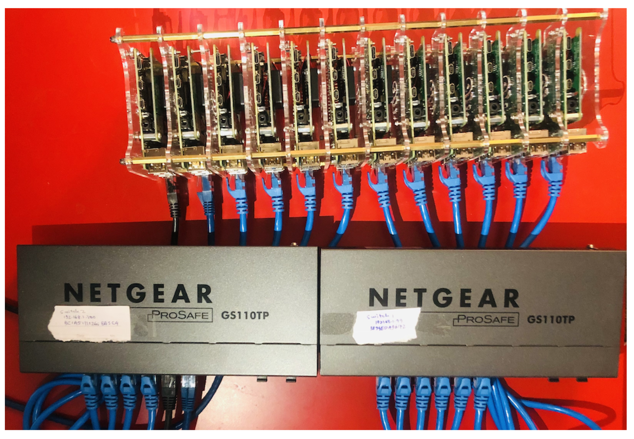
3.1. Cluster Hardware

The Raspberry Pi Foundation (https://www.raspberrypi.org/about/, accessed on 6 May 2022) is a UK based charity responsible for the manufacturing and development of Raspberry Pi boards. The latest board released was the Raspberry Pi Model 4B which uses Broadcom BCM2711, Quad core ARM Cortex-A72 processor with a reported peak performance of 13.5 GFLOPS (http://web.eece.maine.edu/~vweaver/group/green_machines.html, accessed on 6 May 2022), and a Gigabit Ethernet connection, as well as USB, USB-C, and Micro HDMI ports. Users can choose from either 2 GB, 4 GB or 8 GB of RAM—for the purpose of our experiments, we chose the 2 GB variant.

A cluster of 12 Raspberry Pi 4B nodes was built for this study. A standard x86 Linux-based PC (8 core with Linux Mint OS (https://linuxmint.com/, accessed on 6 May 2022) acted as a master node. The computing nodes and the master node were connected through 2 Netgear GS110TP switches. The nodes are powered through Power over Ethernet (PoE) which enables monitoring of their energy usage through the switches internal sensors (cf. Figure 1).

Traditionally, a Raspberry Pi is booted from an image flashed to an SD card. For ease of experimentation and better control over the boot sequence, it was decided to use network booting of a lightweight OS (DietPi) for each node in the cluster. Each client requests the boot instructions from a DHCP server (in this case, the Master node). The DHCP server assigns an IP address to each client and provides boot instructions over the network. When the network is booting, it is common practice to store boot files and the root file-system on the server and have the clients use the Network File System Protocol (NFS) to access files.

3.2. Scientific Workflows

Computational scientists are increasingly using workflows to manage the growing complexity of data intensive simulations and analysis. Workflow technologies are responsible for scheduling tasks, managing dependencies, and staging data for the execution sites [32]. A scientific workflow can be defined as a description of computational tasks and the dependencies between them and is generally described as a directed acyclic graph (DAG), where the vertices represent tasks and the edges represent data or control dependencies [33]. A task in a workflow is defined as the smallest divisible unit of work [34]. Tasks are generally non-interactive executable computer programs performing computation on input data to generate output data. A scientific workflow’s data comprises of structured, unstructured, binary, and text-based data structures [34]. Tasks are blocked until the data becomes available or await completion of all of its preceding tasks.

3.3. Condor Management Software

The cluster management software chosen for this paper is HTCondor [35] or Condor which is a batch job scheduler and resource management system for high-throughput computing on distributed resources. Condor matches jobs with available resources and specialises in check-pointing, recovery and migration of jobs [36].

HTCondor’s Directed Acyclic Graph Manager (DAGMan) is a meta-scheduler for Condor jobs [37]. DAGMan supervises workflow execution and submits tasks which are ready for execution to HTCondor. The main job of DAGMan is to handle the dependencies between the jobs. Jobs are classified into parent and children where child jobs cannot be executed until their parents have completed. In case of failure, DAGMan compiles a rescue graph from which execution can be resumed [34].

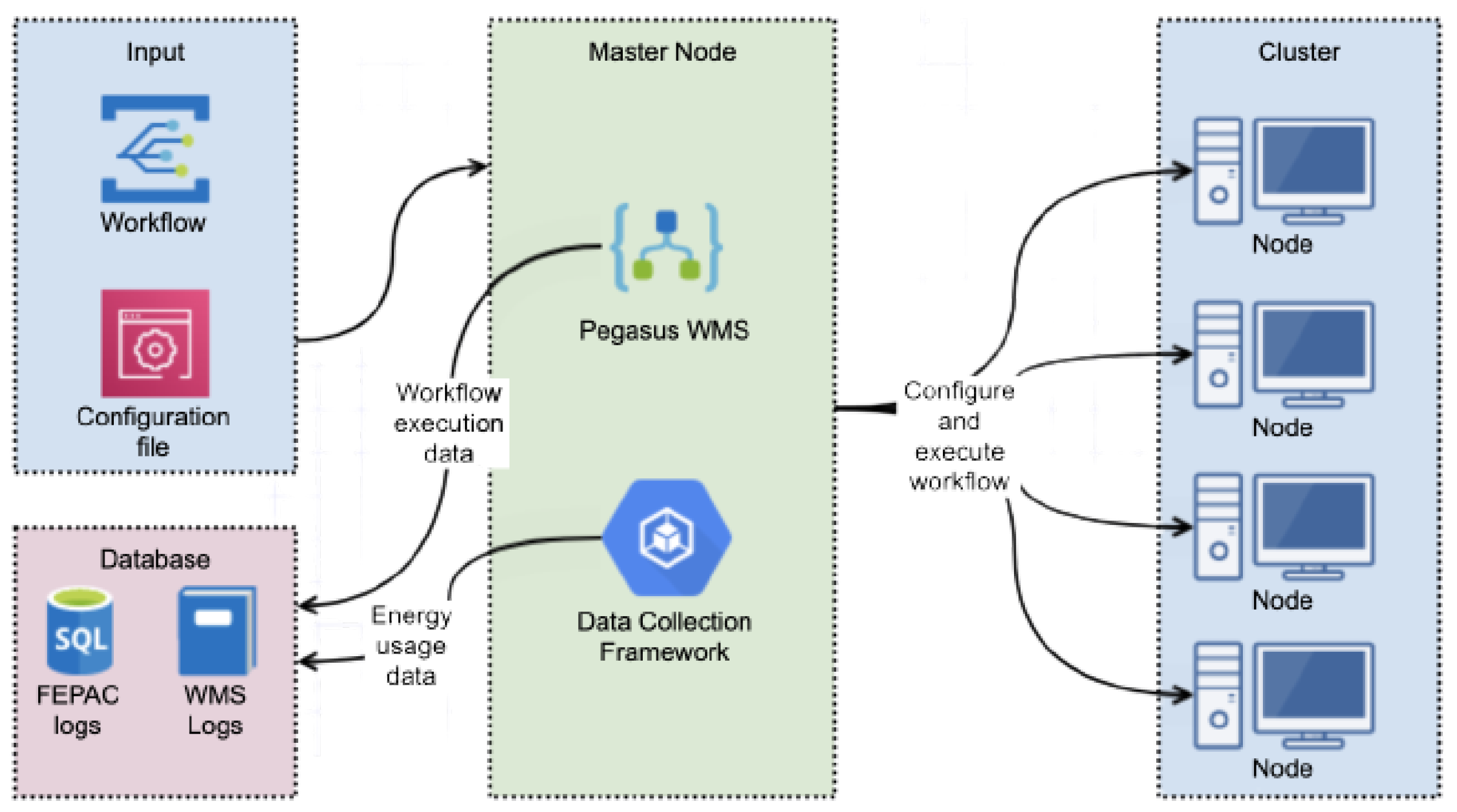
3.4. Workflow Engine

For our work, we chose to use the Pegasus workflow engine, a Workflow Management System (WMS) developed to overcome the shortcomings of DAGMan such as cleanup, set-up of auxiliary tasks and workflow optimisation [2,34]. Pegasus is designed to work on top of DAGMan to overcome these shortcomings and is able to generate a workflow from a metadata description of the desired data product with the aid of artificial intelligence planning techniques [36]. Pegasus uses an XML-based language workflows called dax in which the workflow’s tasks and data are explicitly listed. Pegasus converts this static planning into executable Condor jobs which are then submitted to the DAGMan for execution. Pegasus provides four different scheduling strategies—Random, Round-Robin, Group and HEFT [33]. While Pegasus was designed for executing workflows using grid infrastructures, support for cloud computing has also been implemented [33].

3.5. Experiment Software Setup

Figure 2 illustrates the software setup used and implemented for the purposes of this study. The x86 Linux PC hosted the two main software systems used—FEPAC [14] and Pegasus [2]. FEPAC was previously developed by the authors to monitor the energy usage of parallel computation on clusters as a generic solution for energy monitoring of computation. In contrast, in this work it is used to monitor the energy consumption of scientific workflow execution. FEPAC is used to extract the energy data for each node from the Netgear switches and store it into an MySQL database whereas Pegasus is used to submit and execute workflows on the cluster. Detailed logs from Pegasus assist in pinpointing the time when a particular job of the workflow is being executed and on which node. The energy values in the database stored by the FEPAC framework and the detailed logs generated by Pegasus are cross-linked using the timestamps synced with the master node’s system clock.

4. Astronomy Workflow Energy Evaluation

In this section, we present an in-depth experimental evaluation of the performance and energy consumption of a scientific workflow in the domain of Astronomy on a low-power cluster. The experiments vary the workflow size and cluster size to investigate how different factors affect the performance and energy consumption, respectively. The experiments in this section are based on the experimental setup from Section 3.

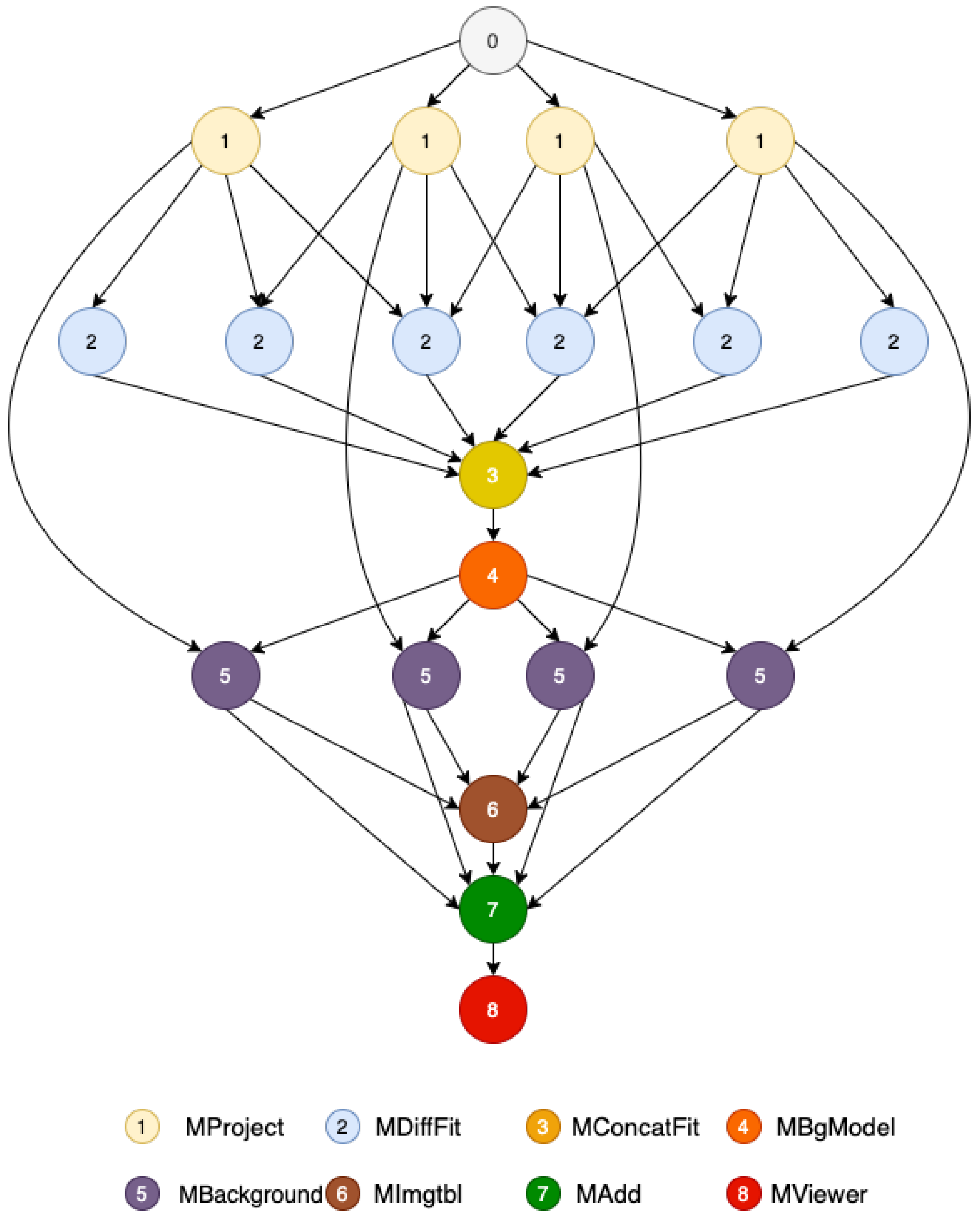
4.1. Workflow Description

The scientific workflow used for the experimental evaluation in this paper is the Montage workflow [38,39]. Montage is a software toolkit used in astrophotography to combine Flexible Image Transport System format (FITS) images of the sky into composite images called mosaics. The toolkit preserves the calibration and positional fidelity of the original input images. A workflow comprising of a number of tasks to develop a relevant mosaic of the sky based on the input parameters is being evaluated in this paper.

Figure 3 illustrates the Montage workflow as a directed acyclic graph (DAG). The Montage DAG has eight levels of jobs which have dependencies from prior levels. For example, the mProject jobs have no dependencies, but prevents dependent mDiffFit jobs from executing until they have finished. Similarly, the mConcatFit job can only be executed once all dependent mDiffFit jobs are completed.

Montage has been classified as an input/output-bound workflow [40] compared to other scientific workflows. However, in our experience, its internal complexity is much more varied, with different job types having different requirements of I/O, memory or CPU. These characteristics make Montage a reasonable representation of more general scientific workflows.

Note that Figure 3 only shows the computation jobs that execute on cluster nodes. To manage the workflow, Pegasus creates many other data transfer and logging jobs that execute before and after each computation job. This evaluation focuses on the main execution jobs as the energy impact on the other jobs are minimal and can be mostly removed with caching.

4.2. Workflow Complexity

The Montage toolkit can be used to generate workflows of varying sizes depending on the requirements of a scientist. The varying size of a Montage workflow is specified in (i) degrees of the sky and (ii) the colour channels which the final images should be generated from.

Table 1. Number of each job vs. Montage workflow size.

Montage Job	Workflow Size
	0.5 Deg.	1 Deg.	1.5 Deg.	2 Deg.
mProject	12	48	108	192
mDiffFit	18	360	1890	6048
mConcatFit	3	3	3	3
mBgmodel	3	3	3	3
mBackground	12	48	108	192
mImgtbl	3	3	3	3
mAdd	3	3	3	3
mViewer	4	4	4	4
Total jobs	58	472	2122	6448

illustrates the number of jobs for different sizes of the Montage workflow. The workflows listed are 0.5, 1.0, 1.5, and 2 degrees; all containing three colour channels of RGB.

Table 1 shows that as the size of the workflow increases, the overall number of jobs also increases. Some of the job numbers remain constant (e.g., mConcatFit, mBgmodel) as these jobs are associated with merging results from other jobs. Other job numbers increase (e.g., mProject, mDiffFit) with an increased workflow size as these jobs are associated with computation that increases as the size of the workflow becomes larger.

4.3. Montage Computation Characteristics

Like any scientific workflow, Montage has specific characteristics to its structure. In particular, Montage has some jobs, such as mProject, that are computationally more intensive than others. Depending on the size of the workflow being executed, there are more of these particular jobs. The combination of the size of workflow and the number of cluster nodes have a direct impact on the job queue time.

To illustrate this, six experiments have been performed by varying the size of the workflow and the size of the cluster. The workflow size is varied from 0.5 to 1.0 and then 1.5 degrees. The cluster size was set to 1 node and 6 nodes, respectively, with each node having 4 hardware threads (for a maximum of 24 hardware threads with 6 nodes).

Figure 4, Figure 5 and Figure 6 illustrate the execution of Montage 0.5, 1.0 and 1.5 degree workflows on 1 node and 6 node low-power clusters. The cluster was setup and data was collected based on the experimental setup detailed in Section 3. The Y-axis in these three figures denotes the execution time (hours:minutes:seconds) of the corresponding workflows.

The graphs illustrates two metrics for each individual Montage job. Job Queued is the time from the job being ready to execute (i.e., its dependencies in the DAG being met) to the time it starts executing. Job Queued measures the delay or queue time due to a temporary lack of resources. Job Executing measures the time the job starts executing until it completes the task and is removed from the cluster.

Figure 4 illustrates that a 0.5 degree workflow has some queuing of the mProject jobs on 1 cluster node (cf. Figure 4a). This is due to the workflow having 12 parallel-capable mProject jobs, but the cluster only has 4 threads to execute them. Consequently, the remaining mProject jobs have to wait until the first one is complete. The remainder of the workflow proceeds as expected. Executing the same 0.5 degree workflow on a 6 node cluster results in no queuing of parallel-capable jobs as there are 24 threads available compared to 12 mProject jobs (cf. Figure 4b).

This is echoed in Figure 5 for the 1.0 degree workflow which shows a large amount of queuing (cf. Figure 5a) when there are a lot less cluster nodes/available threads than jobs. This is a lot more pronounced compared to the 0.5 workflow due to there being 48 mProject jobs vs. 4 threads. For the 1.0 degree workflow, there is even queuing in the 6 node cluster as there are 24 cluster threads vs. 48 mProject jobs.

This pattern is even more pronounced as the workflow size is increased to 1.5 degrees (cf. Figure 6). When there is only a single cluster node, the majority of mProject jobs are queued for a long time; this is due to there being 108 jobs and only 4 cluster threads. When the number of cluster nodes is increased to 6 there is less but still substantial queuing.

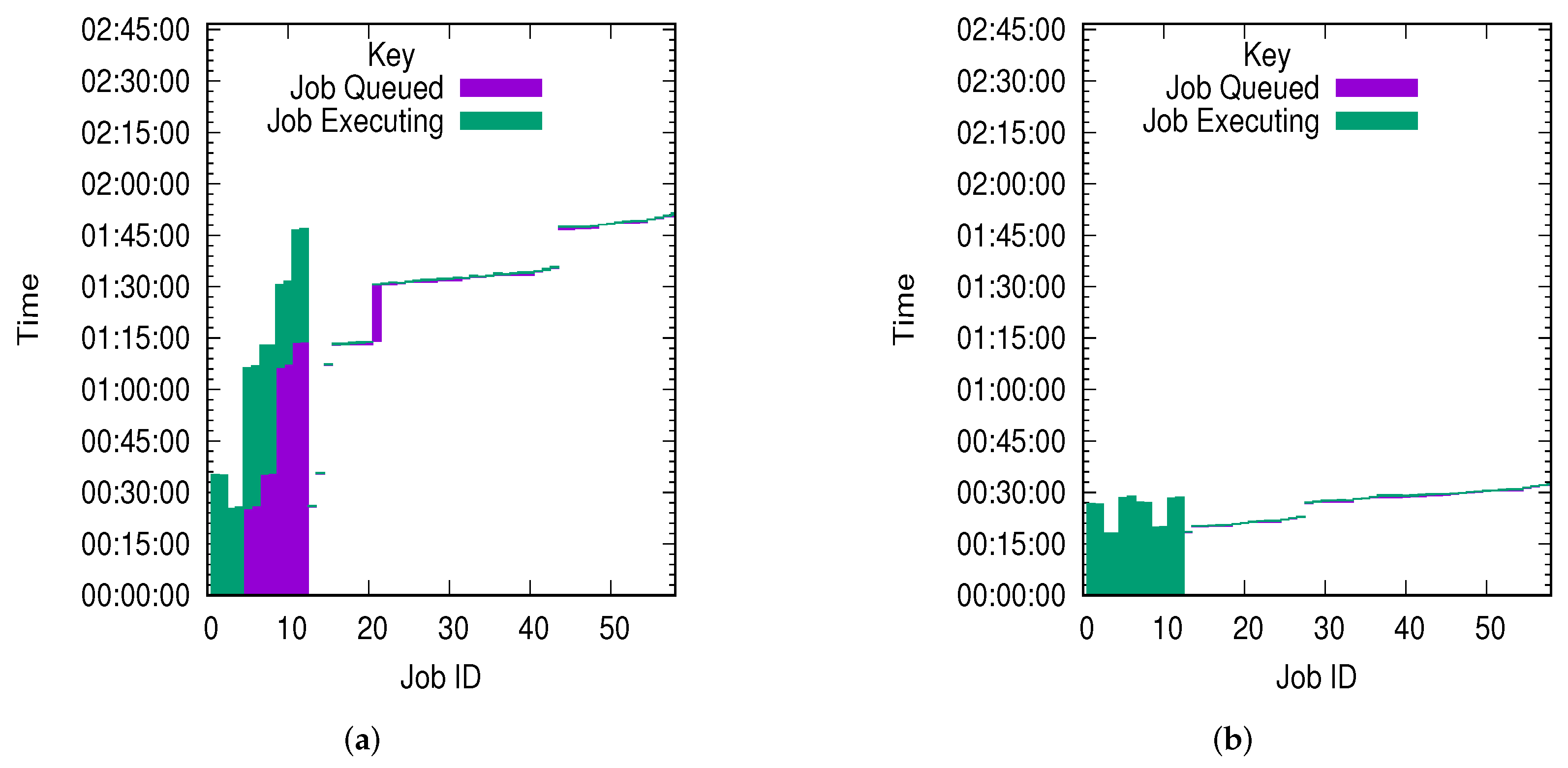
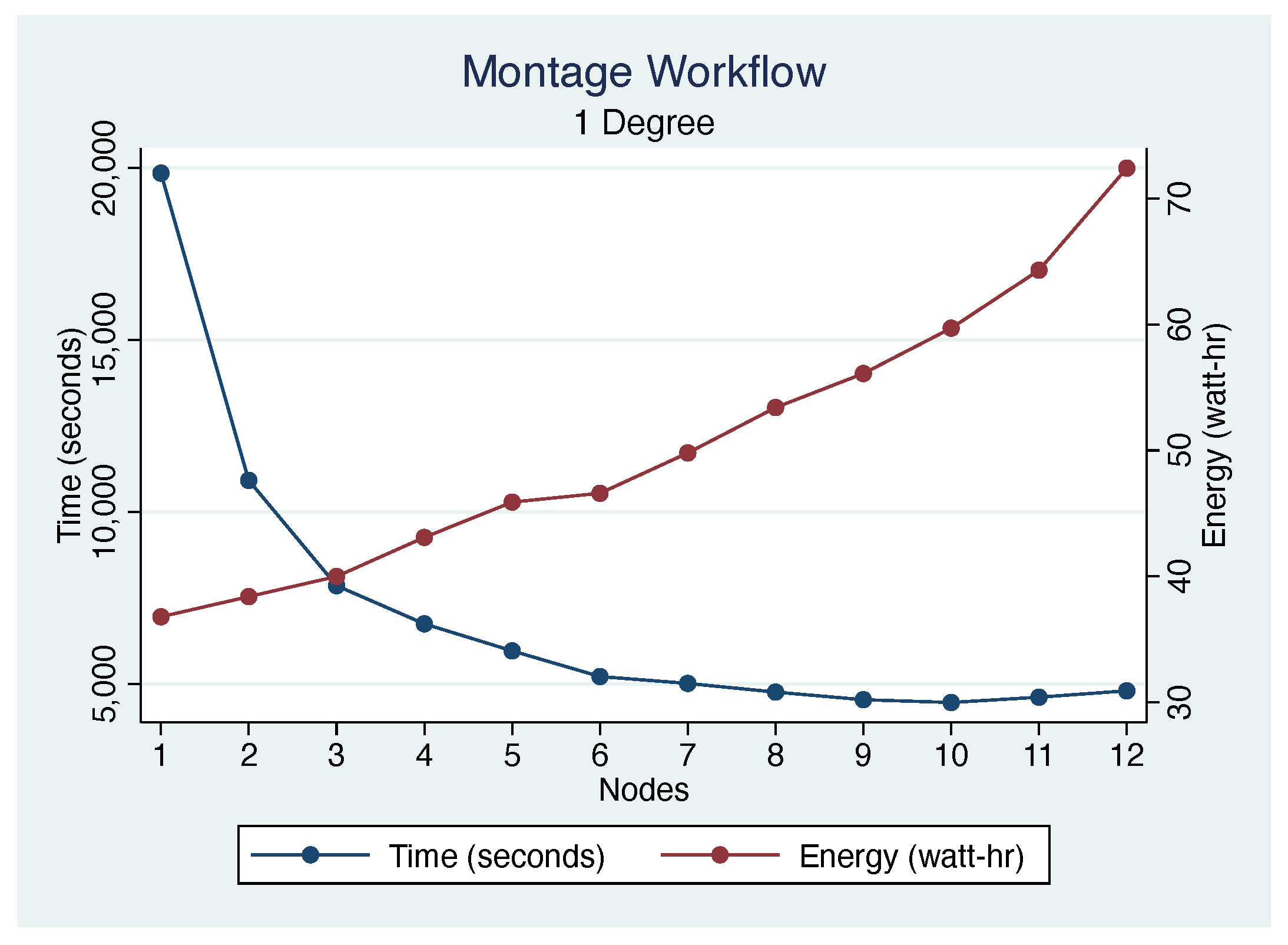
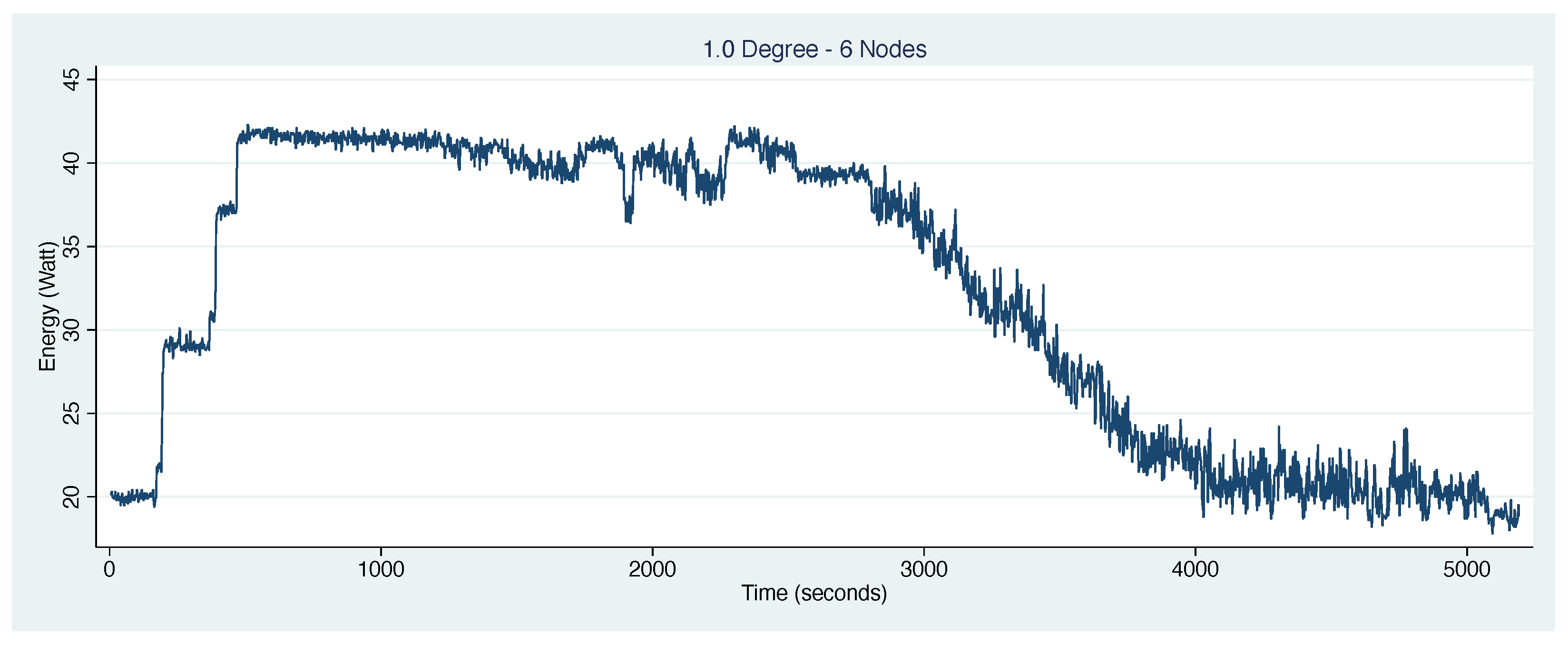
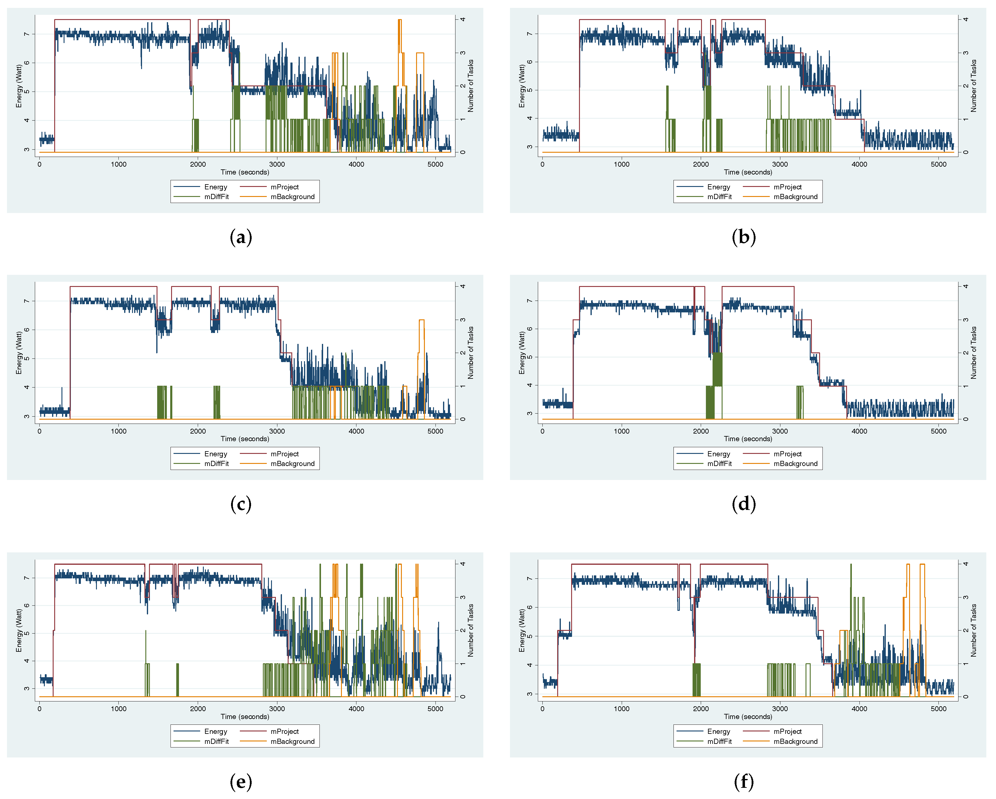
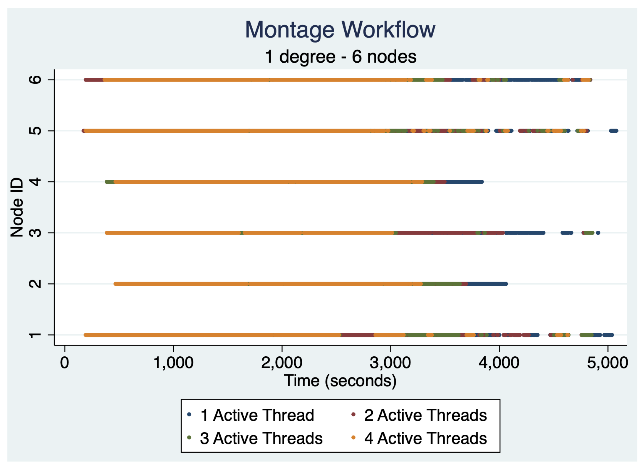
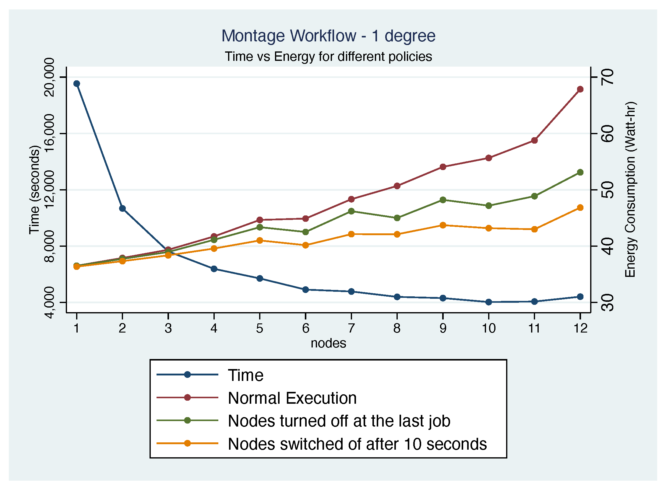
4.4. 1.0 Degree Workflow Results

In the previous section, we showed that Montage workflows provide an interesting and relatively complex workload with which to analyse the computation and energy consumption characteristics of workflows on clusters. In this section, we present the results of experiments for a medium size workflow, Montage 1.0 degrees, with a cluster of 1 to 12 nodes.

Figure 7 illustrates both the execution time and energy consumption of a Montage 1.0 degree workflow on varying sizes of clusters. The left Y-axis is time in seconds from the first workflow job being queued to the last job completing—we do not include any activities on the Master node. The X-axis indicates the number of cluster Nodes from 1 to 12; note that each node has 4 hardware threads, so the number of available threads varies from 4 to 48 in increments of 4. The right Y-axis indicates the total energy consumption in Watt-hours as collected as discussed in Section 3.

The results shown in Figure 7 illustrate that the execution time decreases with more nodes being added. Increasing the cluster size from 1 node to 2 nodes reduces the execution time from 19,544 s (approximately 5 h and 25 min) to 10,675 s (approximately 3 h), hence resulting in a speed-up of $1.83$. However, increasing the cluster to 3 and 4 nodes only reduces the execution time to 7622 and 6384 s, respectively. After 5 nodes (execution time of 5702 s) little reduction in execution time is achieved and the curve flattens out. The maximum speed-up compared to 1 node is $4.81$ achieved with 11 nodes, hence falling considerably short of a linear speed-up.

The reason why the speed-up flattens out is two-fold. First, the more nodes we add the higher the management overhead to trigger job executions and transferring data to/from the nodes. Second, the reduction in execution time largely depends on parallel execution of the computationally intensive mProject jobs. Whereas the median execution time of a single mProject job is around 1500 s (irrespective of the number of nodes used), the other seven job types have a much smaller execution times, with medians of around 65 s (for mBackground) and 15 s (for mDiffFit) for the two job types with a non-constant number of instances. The largest contributing factor to speed-up for the Montage 1.0 degree workflow lies in the parallel execution of mProject jobs—far less gain can be achieved by executing the remaining jobs on an increased number of nodes.

When looking at total energy consumption, it increases steadily in a mostly linear way as the number of nodes increases. A single node uses a total of around 35 Watt-hours, and each additional node adds around 2–3 extra Watt-hours. It should be noted that this is dependent on the length of the execution time, which is reducing with each node being added, as illustrated on the left Y-axis. This is, therefore, illustrating that the main difference in total energy consumption is the overhead for each node. These results illustrate that increasing the number of nodes reduces the total time taken, but also comes at the cost of cluster node overhead, at least for a Montage 1.0 degree workflow.

To further investigate the characteristics of the Montage 1.0 degree workflow execution, Figure 8 illustrates the total energy consumption of the workflow on a 6 node cluster. For each point in time (X-axis), the current energy consumption for all 6 nodes is summed up and presented on the graph. It illustrates that the energy consumption varies significantly over the lifetime of the execution of a single workflow. The initial ‘stepped’ delay is due to the time it takes to obtain the data in the correct location before computation can start. The cluster is being maxed out between 500 and 2800 s by mostly executing mProject jobs. From this point onwards, many job dependencies are being completed and less-CPU intensive jobs are executed, hence there is a reduction in the overall energy consumption. A statistical analysis has shown that there is a strong correlation between the total number of mProject jobs being executed and the total energy consumption (Pearsons correlation coefficient $r=0.995$ with $p<0.01$) but only very weak correlations between energy consumption and the execution of the other workflow jobs.

A further analysis shows that the cluster nodes are not all executing the same workload. Consider Figure 9 that illustrates the energy consumption and jobs split for individual cluster nodes for a Montage 1.0 degree workflow on a 6 node cluster. For each of the sub-graphs, the left-hand Y-axis is the energy consumption at a point in time (used by the blue ‘energy’ line). The right-hand Y-axis is the number of jobs of the three types of Montage jobs (mProject, mDiffFit, and mBackground) at specific points in time. It shows that over the duration of the workflow, the pattern is generally the same, with the larger energy consumption being correlated to CPU-intensive jobs. The later parts of the workflow execution is mostly dedicated to data-aggregation which is distinctly less CPU-intensive and, therefore, uses less energy.

Figure 9 further illustrates that the execution of mProject jobs (the ‘red’ lines in the sub-graphs) is “interrupted” by mDiffFit jobs (the ‘green’ lines in the sub-graphs). This is due to the fact that the scheduling of jobs follows a depth-first strategy that prioritises jobs “lower” in the workflow DAG. Consequently, if mProject and mDiffFit jobs are queued, priority is given to the mDiffFit jobs and they are executed before any queued mProject jobs. This effect is particularly visible for nodes 2 and 4.

4.5. 0.5 Degree Workflow Results

To investigate the energy cost of much smaller workloads on varying size clusters, a series of experiments with a Montage 0.5 degree workflow were performed. As given in Table 1, we have far fewer mProject, mDiffFit and mBackground jobs that need to be executed and, consequently, a much smaller execution time is expected. Figure 10 illustrates the execution time vs. energy consumption result of our experiments with a Montage 0.5 degree workflow.

Similar to the 1.0 degree workflow, we observed a reduced execution time for 2 nodes (4187 s) and 3 nodes (2614 s) compared to 1 node (6696 s), resulting in a speed-up of $1.60$ and $2.56$, respectively. This is mainly due the 12 computationally-intensive mProject jobs being executed on 8 available threads (for 2 nodes) and 12 threads (for 3 nodes). However from 4 nodes onwards, we do not observe a further reduction in the execution time—the execution time remains mostly constant. A closer inspection of the data showed that due to job dependencies, jobs are only ever run on the same 3 nodes and any further available nodes remain inactive during the duration of the workflow execution.

When looking at total energy consumption, it increases steadily in a mostly linear way when more nodes are added (similar to the 1.0 degree workflow). The main difference is that, as discussed above, only 3 nodes are used for workflow execution—the additional nodes run “idle”, but contribute to the overall energy use. The workflow is too small for a cluster of more than 3 nodes and any additional nodes just increase the overall energy used but do not reduce the execution time.

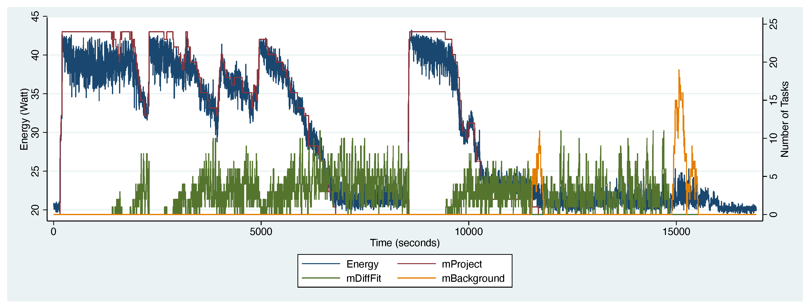
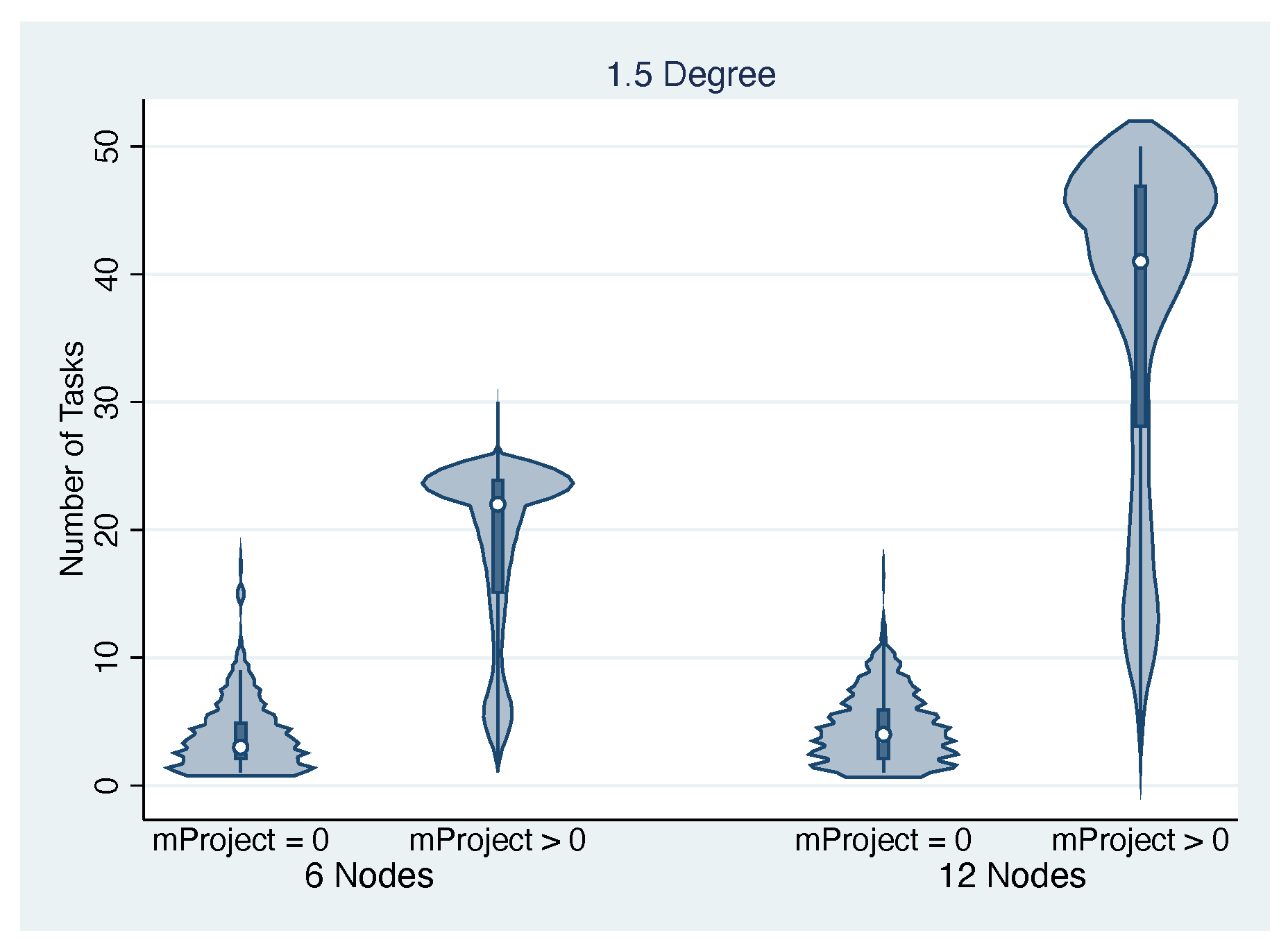
4.6. 1.5 Degree Workflow Results

To investigate the cluster performance for a much larger workflow, a series of experiments with a Montage 1.5 degree workflow were performed. Figure 11 illustrates the execution time vs. energy consumption of a 1.5 degree montage workflow on varying sizes of cluster.

We have a very similar pattern as shown in Figure 7: a speed-up in execution time from 1 node (45,548 s—12 h and 39 min) to 6 nodes (15,868 s), followed by a flattening of the execution time curve with only marginal improvements. The maximal speed-up we observed (for 12 nodes) is $3.34$ compared to the execution time for 1 node. As we have 108 computationally-intensive but parallelisable mProject jobs to execute, we would have anticipated a much better speed-up than what we have observed. Let us look into the reasons for this behaviour in more detail.

Figure 12 illustrates the energy consumption and jobs split for a 1.5 degree workflow on a 6 node cluster. In contrast to Figure 9 where we illustrated the energy consumption and job split for each of the 6 nodes, Figure 12 presents a summation across all nodes. We can clearly see the depth-first execution strategy adopted by the workflow engine by the interleaving of mProject and mDiffFit jobs (starting at 1496 s). The higher priority of mDiffFit jobs results in a complete pause of mProject jobs for several minutes (between 6793 and 8530 s) where only queued mDiffFit jobs are executed. Once they are completed, the execution of the remaining 34 mProject jobs resumes. Montage workflows for 0.5 degree and 1.0 degree did not result in an execution behaviour where mProject jobs were paused across all nodes and for such an extended period of time, respectively.

All mDiffFit jobs depend on the completion of 2 specific mProject jobs only. Hence at 6793 s, many mDiffFit jobs are ready for execution. However, during this period, a median of 4 mDiffFit jobs are executed (a maximum of 10) but there are always many more queued jobs that, based on our interpretation, should be executable. We are yet to fully understand why not more mDiffFit jobs are running in parallel—this is something that requires further investigation as part of future work.

Next, let us consider

Table 2. Montage jobs and their execution patterns on a 1.5 degree workflow.

Activities	1 Node		3 Nodes		6 Nodes		9 Nodes		12 Nodes
Total (seconds)	45,584		22,038		15,868		13,916		13,654
mProject > 0	44,193	96.9%	20,097	91.2%	9787	61.7%	6586	47.3%	5600	41.0%
mProject > 0 running alone	33,791	74.1%	10,362	47.0%	3643	23.0%	1584	11.4%	1918	14.0%
mDiffFit > 0	9774	21.4%	10,176	46.2%	10,217	64.4%	10,153	73.0%	9014	66.0%
mDiffFit > 0 running alone	420	0.9%	724	3.3%	3852	24.3%	4787	34.4%	5044	36.9%
mProject > 0 and mDiffFit > 0	9354	20.5%	9449	42.9%	5970	37.6%	5002	35.9%	3682	27.0%
mProject > 0 or mDiffFit > 0	44,613	97.9%	20,824	94.5%	14,034	88.4%	11,737	84.3%	10,932	80.1%
mBackground > 0	1031	2.3%	970	4.4%	933	5.9%	892	6.4%	860	6.3%
mBackground > 0 running alone	292	0.6%	565	2.6%	688	4.3%	786	5.6%	781	5.7%

, which summarises execution patterns of the three job types with a varying number of instances (mProject, mDiffFit and mBackground). More specifically, the table shows for how many time intervals some of these jobs are running—this gives us an idea of how long it takes, for example, to run all 108 mProject jobs—as well as the percentage thereof of the duration of the entire workflow.

From 3 nodes onwards, we observe an almost linear speed-up for the execution time of all mProject jobs. Hence, the workflow engine does exploit the increasing number of available compute resources quite effectively for mProject. On the other hand, the execution time for all mDiffFit jobs is stable around 10,000 s, irrespective of the number of available nodes. There is less time for mDiffFit jobs to interleave with mProject (the times both types of jobs are being executed together reduces steadily the more nodes are added) and the gain of a faster execution of all mProject jobs is offset by the reduction in overlapping executions—the times when only mDiffFit jobs are executed increase as more nodes are added. As these two job types combined contribute the most towards the overall execution time, this explains the lack of significant reduction in execution time from 6 nodes onwards.

We observed a steady decline in the execution times for all mBackground jobs but not to the same extent as for mProject. Therefore, our experiments for a Montage 1.5 degree workflow showed that only mProject jobs were effectively parallelised when more nodes were added. There was a marginal speed-up for mBackground but a mostly constant execution time for mDiffFit, respectively.

This is further illustrated in Figure 13. We show the number of active jobs (or tasks) when at least one mProject job is running (i.e., mProject > 0) compared to the number of active jobs when no mProject job is running (i.e., mProject= 0), for both 6 (maximum of 24 threads) and 12 nodes (maximum of 48 threads), respectively, in the form of a Violin plot. Figure 13 clearly shows that the workflow engine gets close to using up all available compute threads when mProject jobs are being executed (Median of 22 and 41 for 6 and 12 nodes, respectively) but fails to do so when no mProject jobs are running (Median of 3 and 4, respectively). As the execution time for all mProject jobs gradually decreases the more nodes are added, more and more the cluster becomes underutilised.

Apart from mProject, none of the Montage jobs effectively uses the available resources. Fewer nodes are active outside mProject execution. For a both a 6 and 12 nodes cluster, 3 nodes would suffice about 70% of the time with 4–5 nodes required for the remaining 30%. This explains the almost linear increase in the total energy consumption (cf. Figure 11)—additional nodes are used extensively whilst mProject jobs are running, but are either used scarcely or not at all otherwise. They still contribute to the overall energy consumption even when running “idle”—an energy-aware scheduler could either switch these nodes off or make them available for other users.

As part of future work, we will investigate why the workflow engine cannot execute more mDiffFit and mBackground jobs in parallel. Increased parallelism for these two job types could lead to improved utilisation of the cluster, a reduced execution time in the order of 20% to 30% for larger Montage workflows and, consequently, a better energy usage footprint.

4.7. Discussion

An experimental evaluation of the Montage workflow execution on a small board compute cluster was presented in this section. Analysis of data produced through these experiments has unveiled some interesting results which are discussed in the remainder of this section.

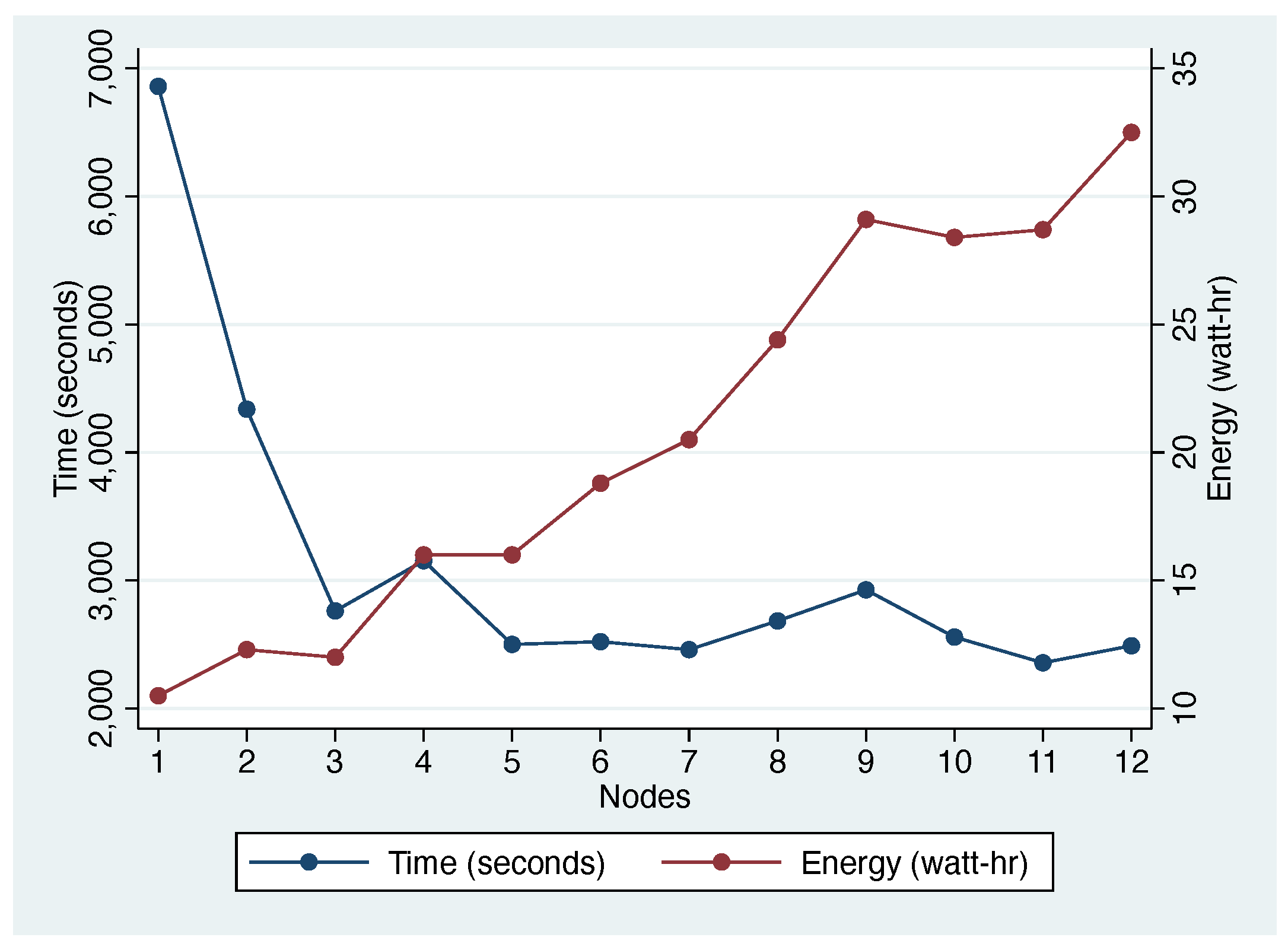
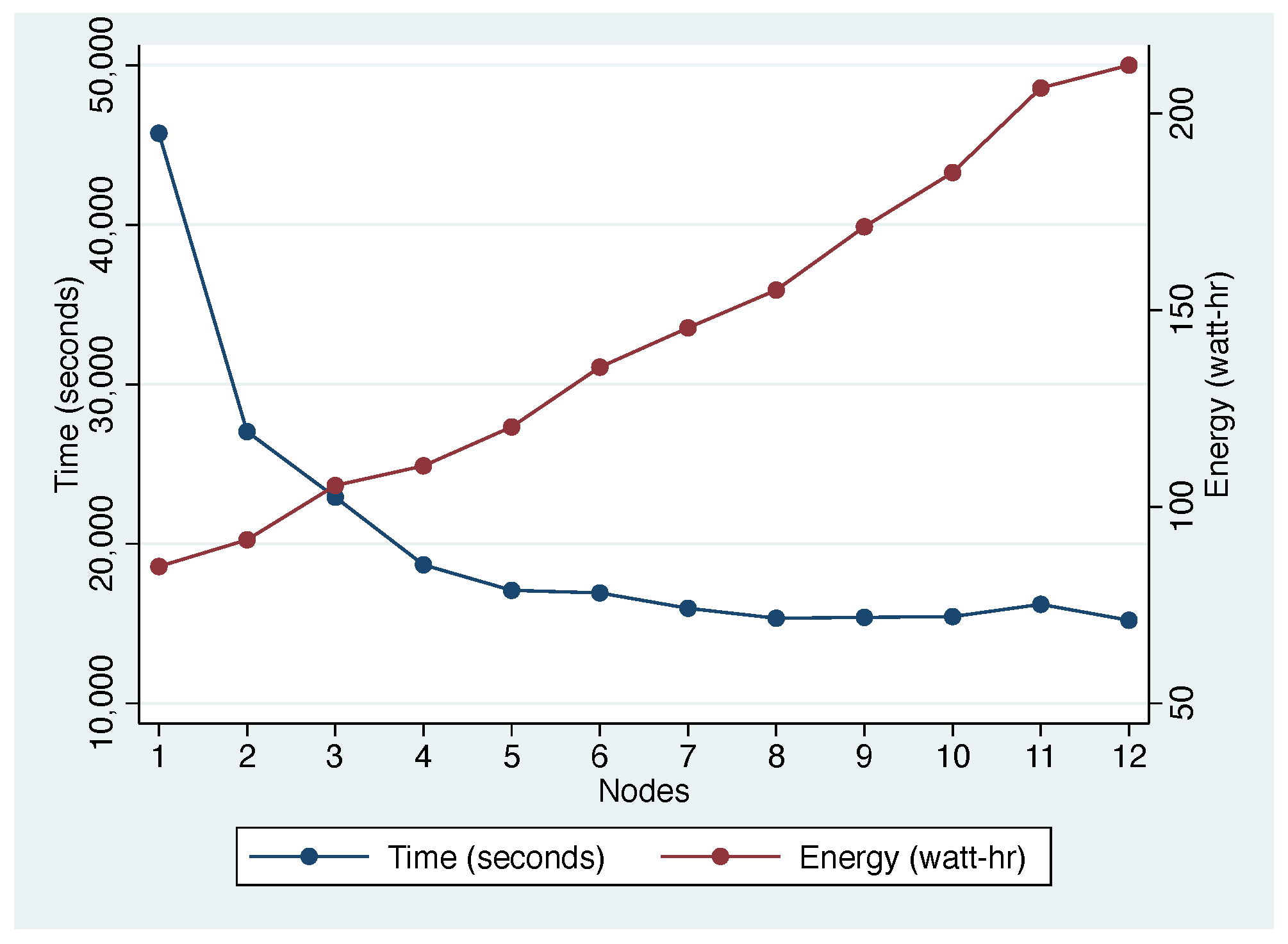
4.7.1. Impact of Cluster Size

The presented experiments have shown that, as expected, increasing the cluster size has a significant impact on the computation time for workflows with many parallelisable jobs. Increasing the size of the cluster from 1 node (4 threads) to 2 nodes (8 threads) will result in an almost halving of the computation time (ie linear speed-up). This pattern generally holds for all workloads, and extends to 3 and 4 cluster nodes. These gains due to increasing cluster size does not continue past around 5–6 cluster nodes (20–24 threads) for the chosen workflows though. Increasing the number of cluster nodes beyond this has a small impact on the overall computation time of the workflow. This is the case even with large workflows with a large number of parallelisable jobs. This pattern can generally be attributed to a number of factors, including increasing dependencies between workflow jobs, the overhead of coordinating more cluster nodes, and the increased data transfer needed, respectively.

We conclude that, for any workflow that requires some level of coordination and/or synchronisation amongst jobs, there will be a point were adding further compute nodes will only result in a marginal reduction in computation time.

4.7.2. Impact of Cluster Configuration

The experience of configuring and analysing various cluster configurations has shown that there are many factors that effect computation performance and energy. Configuring a cluster to be efficient requires a lot of effort. In this paper, the experiments used the default configuration for Condor and effort was made to minimise the data transfer needed for jobs to execute. As all nodes where configured using NFS, minimising transfers had a large impact on the overall performance. Experiments have shown that when considering energy, the overhead of running nodes has the biggest impact for larger cluster sizes as there are diminishing returns with regards to run-time performance.

From our experiments we conclude that for most energy efficiency, it is best to either use a node to the maximum or have this node not present at all. Consequently, this may require further work in adjusting workflow scheduling in order to make them more “energy aware”.

4.7.3. Impact of Workflow Structure

The results presented in this paper show that the greatest impact on the workflow execution time is the structure and size of a workflow. Increasing the size of the workflow will increase the workload and the amount of computation required. However, increasing the workflow size also increases the number of jobs that integrate and, therefore, depend on the results from previous jobs. Overall, when profiling jobs, the most important are computationally intensive jobs as these not only require the most computation, but also delay dependent jobs the most.

4.7.4. Performance vs. Energy

The focus of this paper is analysing the impact on performance and energy of varying sizes of clusters and workflows. The expectation was that there would be a trade-off between performance and energy consumption. Although this has been shown to be true for small sizes of cluster, this does not continue for larger sizes of cluster. For larger cluster sizes, regardless of workflow size, increasing the number of nodes does not continue to improve the performance of workflows beyond a threshold. As illustrated in Table 2, adding further nodes to our 12 node cluster will not result in an improvement of the overall run-time performance for a Montage 1.5 degree workflow. We stipulate that a similar pattern will emerge if we increase the Montage workflow to 2.0 degrees and beyond.

5. Bioinformatics Workflow Energy Evaluation

In this section, we present an experimental evaluation of the performance and energy consumption of a scientific workflow in the domain of Bioinformatics on a low-power cluster. The experiments vary the workflow size and cluster size to investigate how different factors affect the performance and energy consumption, respectively. The experiments in this section use the experimental setup as described in Section 3.

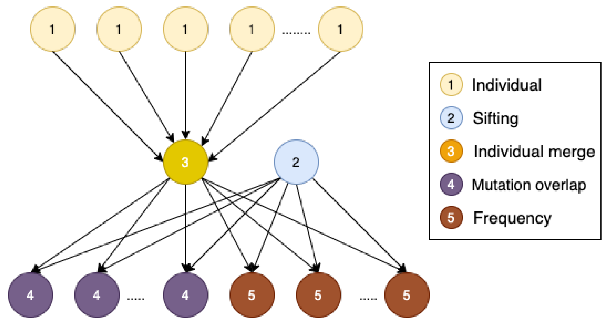
5.1. Workflow Description

The Bioinformatics workflow used for the experimental evaluation in this section is based on the data collected by the 1000 Genomes Project [41,42]. The purpose of this workflow is to analyse the data and cross-match the whole datasets for mutations. The workflow also identifies mutational overlaps in order to evaluate potential disease-related mutations. The extracted data, along with the mutation’s sift scores (calculated by the Variant Effect Predictor [43]), can help researchers in discovering the exact mutation which is the cause for a certain disease in a person. The workflow also provides visualisation of the data for easier understanding and future analysis, respectively.

Figure 14 illustrates a directed acyclic graph (DAG) of the Bioinformatics workflow being evaluated in this section. The DAG has three levels of jobs which have dependencies from prior levels. For example, the individuals jobs have no dependencies, but prevent the dependent individual_merge jobs from executing until they have finished. Similarly, a frequency job can only be executed once all dependent sifting jobs are completed. Similar to Section 4, Figure 14 only shows the computation jobs that execute on cluster nodes and not the jobs that are running on the master node.

5.2. Workflow Complexity

The Bioinformatics workflow used in this paper uses seven sets of population data to calculate, analyse and report on the different relationships between individuals and genetic variation. The workflow generates a wide range of plots and co-relation data for easy analysis by the researchers. The workloads are categorised on the size of population data that the workflow computes on.

Table 3. Number of each job vs. Bioinformatics workflow size.

Bioinformatics Workflow	Workflow Size
	Small 10 k Data	Medium 20 k Data	Large 30 k Data
individual	50	50	50
sifting	1	1	1
individual_merge	1	1	1
frequency	7	7	7
mutation_overlap	7	7	7

illustrates the different number of jobs for different sizes of the workloads.

The parallelisable individual jobs can be set depending on the resources available. Most of the experiments conducted in this paper set the number of individual jobs to 50 so as to accommodate for maximum resources available (12 nodes, 4 threads each = 48 parallel jobs). Apart from the individual jobs, the number of jobs for the Bioinformatics workflow do not change in relation to the size of workload.

The frequency and mutation_overlap jobs are dependent on the demographic data (population cohorts). As the whole 1000 Genome Project consists of data from seven populations, the number of these jobs are always constant to seven for each chromosome and for any size of workload. The sifting and individual_merge jobs are always one for each chromosome as the individual_merge job requires output of all individual jobs to be able to merge them into one single data. Moreover, the sifting job is independent of the whole workflow and can execute on its own without the need to parallelise.

5.3. Workflow Characteristics

The Bioinformatics workflow has many characteristics which are specific to the workflow. In particular, there are two different input variables that can be controlled by the user—the size of workflow (the data to be computed) and the number of parallel jobs. Depending on the user’s need and the resources available there can be more or less of these jobs. The combination of the number of jobs and the size of workflow directly relates to the queuing of the jobs, the execution time, and the energy consumption of the workflow.

The computing nodes used in this experiment have 2 GB of RAM available on them. The workflow loads the whole data-set into memory. This meant that the workflow was limited by the memory capacity of the nodes. After removing the memory used by the OS and other necessary processes, we are left with 1.6 GB of RAM for computation. This translates to less than 400 MB of RAM for each thread in the computing nodes. This was the highest limit of data that the workflow could process. After analysis of the data, it was found that 1 MB of data was equal to 100 lines of individual data in the file. After testing a few different sizes of workload, the sizes of data to be used in experiments were finalised to 10 k for small workload, 20 k for medium workload and 30 k for large workload. Any data bigger than 30 k or 320 MB would crash the workflow.

5.4. Bioinformatics Workflow on a Single Node—Results

The results of varying the number of parallelisable jobs on a single node cluster for a large workflow (30 k data) are presented in this section. This is mainly performed to showcase the optimal number of parallel jobs to be executed on a single node when comparing the time of execution with the energy consumption of the workflow.

Figure 15 illustrates both the execution time and energy consumption of a large workload Bioinformatics workflow on varying numbers of parallel jobs. The left Y-axis denotes time in seconds and the right Y-axis indicates the energy consumption used by the node for the duration of the execution. It is important to note that the energy data does not take into account the energy of the master node. The X-axis indicates the number of parallel jobs being queued on the node.

The results shown in Figure 15 illustrate that the execution time decreases with the number of parallel jobs until all 4 threads are being used. The time decreases from 40,595 s (approximately 11 h and 16 min) to 12,821 s (approximately 3 h and 33 min), hence resulting in a speedup of 3.16. As it can be seen, the energy consumption closely relates to the number of jobs being executed. After four jobs, the time and the energy consumption deteriorates from 12,821 s (approximately 3 h and 33 min) to 19,721 s (approximately 5 h and 28 min) which is a 53% increase. Similar results can be found for energy consumption as well.

The major reason for this observation can be that a node only has 4 hardware threads for parallel computation and any jobs more than four leads to queuing and higher overheads of scheduling jobs, transferring files and merging. The optimal performance of the nodes in a cluster can be achieved when the number of jobs to be scheduled on any node equals the number of hardware threads available [14]. This is also illustrated in Figure 15 and concludes that to achieve the sweet spot between energy consumption and execution time, the computing power of a single node needs to be completely utilised before scheduling jobs on any other nodes.

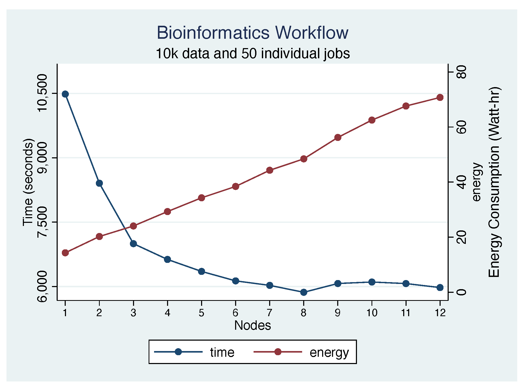
5.5. 10 k Workload Results

To investigate the energy consumption of a small workload on varying size of cluster, a series of experiments with varying data sizes were performed on the Bioinformatics workflow. As seen from Table 3, the number of jobs do not change as compared to any other workload but the amount of computation by each job increases when the workload increases. In this section, we present the results of the Bioinformatics workflow with a small sized workload (10 k data with 50 individual jobs) being executed on 1 to 12 nodes.

Figure 16 illustrates both the execution time and energy consumption of a Bioinformatics workflow with 10 k data workload on varying size of cluster. The left Y-axis is the execution time in seconds. The right Y-axis is the energy consumption of the nodes in Watt-hours collected as discussed in Section 2. The X-axis indicates the cluster configuration, i.e., how many nodes were used to compute. Moreover, no jobs on the master node were considered as they were mainly folder creation and file transfers.

The results shown in Figure 16 illustrate that the execution time decreases with more nodes being used for computation. This is expected as more computation power should result in faster workflow execution. The lowest execution time in the experiment was recorded for 8 nodes as 5866 s (approximately 1 h and 37 min) which was 44.05% lower than that of 1 node (10,484 s; 2 h and 54 min).

A steady increase in energy consumption was observed similar to Section 4. A single node used around 14.34 Watt-hours during the computation and every additional node increases the energy consumption by around 4.5 Watt-hours. As the energy consumption takes into account the execution time of the workflow, the difference between the energy consumption between two nodes is due to the increased overhead of computing on additional nodes. The results illustrate that faster execution of workflow by increasing the number of nodes comes at a cost of increased energy consumption. This led to further investigation on finding the sweet spot between execution time and energy consumption. Reasons for the increased energy consumption and ideas to reduce it were also discussed.

The increase in energy consumption is almost linear and further investigation into the data shows that the reason for the increase is totally different than that found in Section 4. The linear increase is a result of just 1 thread being used and the majority of the nodes being idle during the execution of individual_merge job. As illustrated in Figure 14 and Figure 17, individual_merge job acts as a bottleneck for the workflow and the workflow cannot proceed further unless the job has been completed. This job utilises just 1 thread out of all the computing power available. Due to this, during the execution of this job, most of the nodes are idle. They still contribute to the total energy consumption of the cluster but do not help in the workflow execution.

Further analysis showed that, for 1 node execution, the individual_merge job was being executed for 4032 s (approximately 1 h and 7 min) while the total execution time was 10,484 s (2 h and 54 min) for the workflow. This meant that for almost 38.45% of the execution time, the majority of the cluster was idle and consuming energy without contributing to the computation. The results become more prominent as we increase the number of nodes. The total execution time for a 12 node cluster is 5976 s (approximately 1 h and 39 min) and individual_merge job monopolises 4132 s (approximately 1 h and 8 min) for itself. This results in the majority of the cluster being idle for 69.15% of the time.

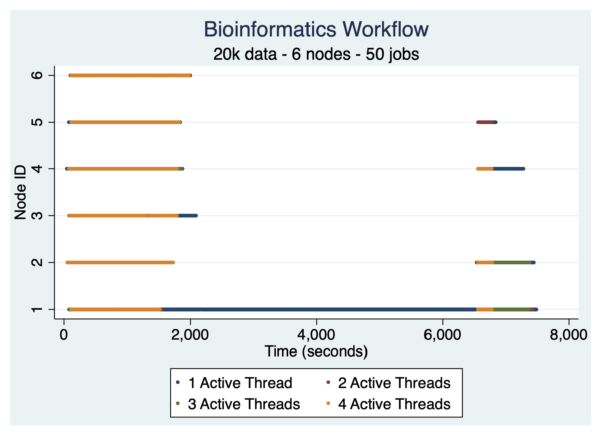
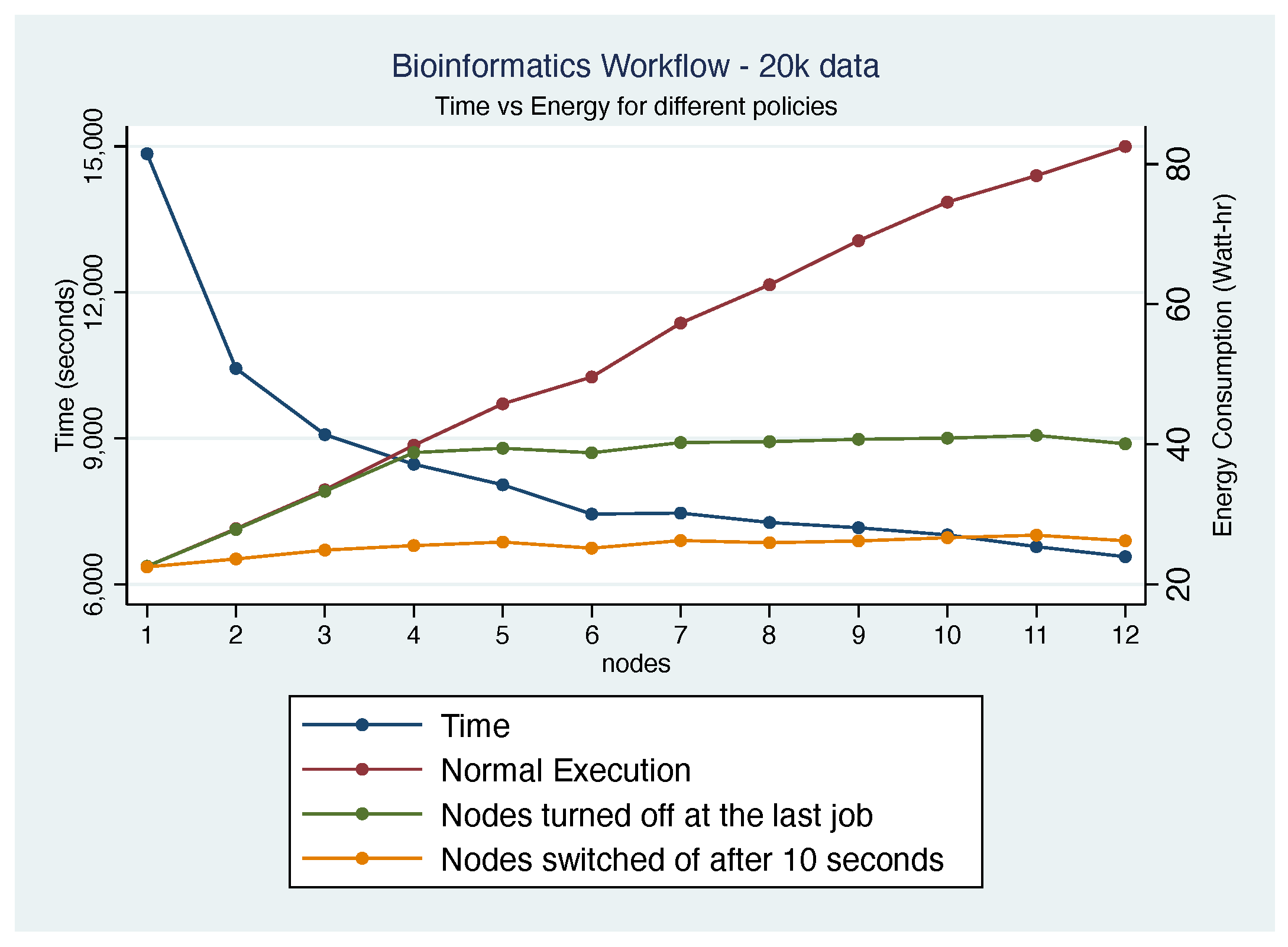
5.6. 20 k Workload Results

An investigation of a medium size workload on the Bioinformatics workflow was conducted using 20 k data points. As given in Table 3, the number of jobs stays the same for this set of experiments but the work performed by each job increases by 100% as compared to the small workload.

Similar to Figure 16, a reduction in the execution time of the workflow was observed when more nodes were added. The execution time gradually decreases till 12 nodes. The maximum difference of 55% increase in time between the 1 node execution (14,924 s—approximately 4 h and 8 min) and the 12 nodes execution (6645 s—approximately 1 h and 50 min) was 8279 s (approximately 2 h and 17 min), resulting in a speed up of approximately 2.25. When analysing the total energy consumption, similar patterns as shown in Figure 16 were seen in this experiment. Energy consumption increases by 267.9% for 12 node execution when compared with 1 node execution. This increase is observed as the reduction in the execution time does not compensate for the increase in the averaged energy consumption of the cluster when a new node is added.

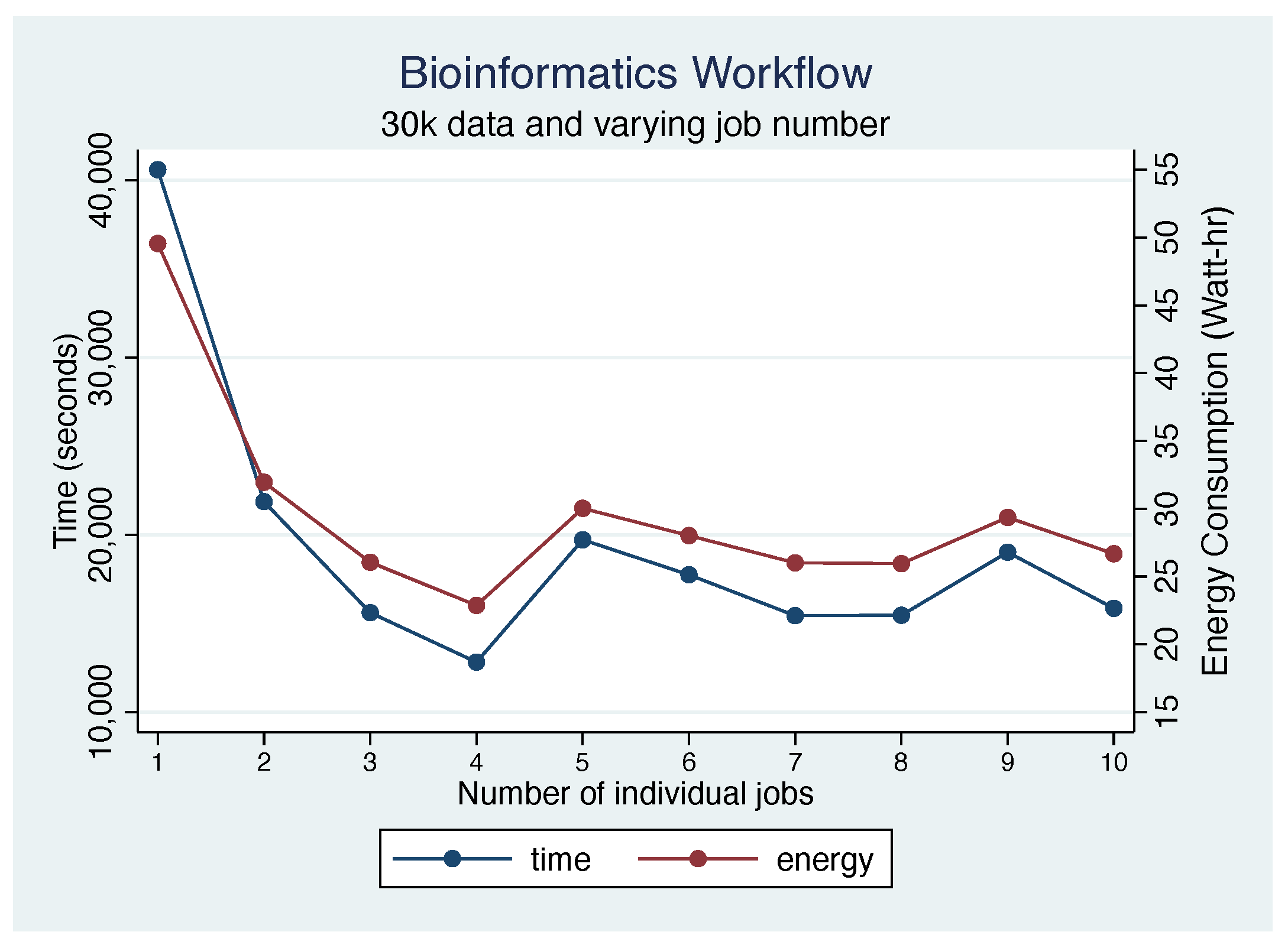
5.7. 30 k Workload Results

To further investigate the performance of the Bioinformatics workflow, a series of experiments were performed with a large workload of 30 k data points. As the number of jobs was the same, this means the computation for each job increased by 200% as compared to the smaller workload.

A steady decline in the execution time is observed between 1 node (19,013 s—approximately 5 h and 16 min) and 7 node (7740 s—2 h and 9 min). A speed-up of 2.45 or a 59.3% decrease in the execution time was achieved from these experiments. After node 7, the execution time stabilises and only 5–6% variation between the execution times is observed. The energy consumption of the experiments followed the same reasoning as Figure 16. The nodes are idle for the majority of the time and this leads to the idle energy consumption values tainting the actual energy consumption of the cluster during the computation.

5.8. Discussion

An experimental evaluation of a Bioinformatics workflow has been presented in the previous sections. The data obtained from these experiments presented a number of discoveries and results regarding the workflow and how it is executed. These results are discussed in the remainder of this section.

5.8.1. Impact of Cluster Size and Configuration

The results presented show that the cluster size and configuration significantly impact the execution time of the workflow. Generally, increasing the size of the cluster from 1 node (4 threads) to 2 nodes (8 threads) will result in an almost halving of the computation time but due to the particular characteristics and the bottlenecks of the jobs in this workflow, a non-linear speed-up was observed for the different workload executions. For example, increasing from 1 node to 2 nodes resulted in a 19% and 29% decrease in execution time for 10 k and 20 k data workload, respectively. Similarly, a 35% decrease is observed for 30 k data workload.

The gains obtained are marginal and not prominent past 5–6 cluster nodes (20–24 threads) for the chosen workflow. This can be due to a large number of factors, including increased overheads, dependencies, data transfer, etc. As for the energy efficiency of the cluster, efforts were undertaken to reduce the data transfer and dependencies of the jobs without affecting the underlying workflow or condor configurations. These proved to be unfruitful as the gains were quickly diminished by the bottlenecks inherent to the workflow. These are discussed in the next section.

We conclude that for any workflow to maximise the execution time and energy efficiency, it is best to utilise all the available computing power of a single node before scheduling jobs on other nodes. A workflow with inter-dependent jobs will always come to a point when adding more computation power will result in a very small increase in performance. Moreover, for any workflow with a bottleneck, further work is required to make it “energy aware”. This can include altering the scheduling of the jobs, changing the default dependencies, changing the cluster configuration, etc.

5.8.2. Impact of Workflow Structure

The workflow structure has a huge impact on all the aspects of its execution. A poorly implemented workflow can be very inefficient leading to long execution times and wasted resources. In this paper, the Bioinformatics workflow has a constant number of jobs for any workload. This meant that increasing the workload led to a direct increase in the computation required. A spike in the energy usage of the cluster is observed when a computational job is being executed.

The results presented in this paper show that there is a huge bottleneck during the execution of a single job in the Bioinformatics workflow. This leads to a delay in the dependent jobs which results in a waste of energy and computing resources. This bottleneck can be removed by energy-aware execution and scheduling of the workflow. This will require changes to the workflow and the underlying scheduler. These changes and their gains are beyond the scope of this paper and will be researched in future.

5.8.3. Performance vs. Energy

The experiments performed in this section present the impact of varying sizes of cluster and workflow on the performance and energy consumption of the workflow. The expectation was that there would be a gain in performance of the workflow at an expense of the energy consumption. This was observed to be true but an in-depth analysis of the workflow showed that there is a way to optimize the workflow in order to gain more energy savings or execution time. For larger cluster sizes, no considerable performance gain was observed for the increase in energy expenditure. We stipulate that similar results will be observed on the execution of the Bioinformatics workflow with different workloads.

5.9. Results Compared to the Literature

In this paper, the approach taken is to analyse the energy usage of the workflow as a whole. This is in contrast to [44] which focused on the individual jobs and the factors affecting their execution. Results were consistent between both approaches with both identifying that execution can be optimised for energy without a huge reduction in performance by identifying and reducing the overheads and dependencies between the jobs.

The workflows chosen in this paper reflect two distinct areas of scientific computing and have different computational characteristics. Montage is I/O intensive and Bioinformatics is CPU intensive [45]. There is not much overlap between these domains and hence the results obtained can be considered relatively generic. Refs. [46,47] follow a similar approach in which they analyse two different workflows with different characteristics to provide conceptual results that can be applied generically to any workflow executions.

In this paper, we perform experiments based on varying the size of the workflow and therefore the workload. This is performed mainly to analyse the effect of execution time and energy consumption of varying complexities. Refs. [48,49] focus on executing three workflows on a single cluster configuration. Their results are similar to the ones obtained in this study. Our study expands on these previous studies by varying the configuration of the cluster and the workflows. This provides a comprehensive set of results which can help generalise the concepts to multiple workflows.

We have performed a detailed analysis of the computation/energy characteristics alongside analysing the detailed structure of the workflow. Ref. [50] focuses on the structure of workflows along with the inter-dependencies of the jobs to find the trade-off between make span and cost. Analysing the workflow as a whole along with its structure has allowed us to understand the workflow in depth and similar factors affecting the performance and energy of the workflow.

6. Energy-Aware Workflow Execution

The results from previous experiments motivate a need for energy-aware execution of workflows on compute clusters in order to result in better trade-offs between run-time performance and energy consumption. In this section, we further support the cause through detailed analysis of the workflows and proposing policies which can act as a rule base on development of a novel energy-aware workflow execution software/scheduler. We show that the policies, when implemented, can help in reducing the energy footprint of the workflows by theoretically implementing them in our experiments.

6.1. Workflow Analysis

To complement what was concluded in Section 4 and Section 5, we investigated the number of active threads per node during the execution of the workflows as a measure of how much the resources of the cluster are being utilised (cf. Figure 17 and  Figure 18).

For both figures, usage of all 4 threads is indicated by ‘orange’ dot and usage of 3 threads is indicated by ‘green’ dot. ‘red ’ and ‘blue’ colored dots are used to indicate usage of two and one threads, respectively. The y-axis denotes the individual node and the x-axis the timestamp at any given instant. The analysis only considers the jobs which were executed on the nodes and not the local jobs such as file/folder creation, file transfers, etc.

For the Montage workflow, we analysed the 1 degree workload on a 6 node cluster. During the first part of workflow execution where mostly mProject jobs are executed, each node uses all 4 available threads. However, in the second part of the execution (i.e., post mProject), neither 4 nor 3 threads were being used completely, but most nodes have only two or even one active threads.

For the Bioinformatics workflow, a workload of 20 k data was provided to the workflow to be executed on 6 nodes. As expected, during the execution of individuals jobs, all threads from all nodes were being used and the number of jobs exceeds the number of available threads. However, during the second part of execution, only 1 thread was being utilised. This job individual_merge takes up the majority of the workflow execution time in which most of the nodes are idle. During the third part of workflow execution, 4 nodes are being utilised with a mix of 3 and 2 threads each.

We are yet to fully understand the execution behaviour of these two workflows as there are instances when the jobs could be queued better in order to save more energy or time. For example, during the second part of the Montage workflow, the 17 jobs to be executed which could have been been scheduled on just 4–5 nodes and 1 node could have been turned off to save energy. Fine grain analysis of the job dependencies, scheduler settings, etc., is required to further understand and explain a particular execution of workflow.

In conclusion, using a set of rules (or “policies”) to govern the execution of jobs and the configuration of cluster can help improve the energy consumption of the workflow. These policies can vary in a wide range from scheduling jobs on particular nodes to changing the configuration of the cluster based on the energy budget of the workflow, respectively.

6.2. Optimising Energy Usage

To investigate the actual impact of the different policies, we analysed the execution data of one use case of each workflow. These policies are explained further in this section. The analysis of the data can be seen in Figure 19 and Figure 20).

The workload being used to compare between the policies for Montage and Bioinformatics workflows are 1.0 degree and 20 k data, respectively. For both figures, the x-axis denotes the number of nodes. The left and right y-axis denote the execution time of the workflow and energy consumption for the particular policy, respectively.

The “maroon” colored line depicts the energy consumption when the workflow is executed normally as their authors intended it to be. There is no changes made to the workflows. The “green” line denotes the execution of workflow in which the nodes are turned off at the end of their last job. This includes the idle time in between the first job and the last job on each node. Finally, the “yellow” color line shows the energy consumption when the policy to turn nodes off after 10 s of inactivity is applied. This gives us a lower bound of energy consumption as we do not incorporate the impact of re-starting nodes (if required). This analysis only considers the jobs which were executed on the nodes and not the jobs on the master node such as file/folder creation, file transfers, etc.

In the case of Montage, our experiments have shown that the “optimal” number of nodes is not a constant and may vary during the execution of a workflow (as is shown Figure 18). An intelligent scheduler could exploit this and use fewer nodes for parts of a workflow execution without impacting overall run-time performance. This can reduce the energy consumption as shown in Figure 19.

For a Montage 1.0 degree workflow on 6 nodes, for example, if we excluded the impact of nodes 2 and 4 once they become inactive (cf. Figure 18), we would get a reduction of approximately 10% in overall energy consumption. For a Montage 1.5 degree workflow on 12 nodes, a similar exclusion of inactive nodes would result in an approximate 25% reduction. Figure 19 shows the same and can help in identifying the optimal cluster configuration and execution time. The maximum reduction in energy consumption that was seen during our experiments was 30% for 12 nodes.

The Bioinformatics workflow has a single process that runs on its own for a considerable amount of time with all other nodes being inactive. Some of these nodes will be needed again in the third part of the execution. This property of the workflow can be exploited and can lead to significant savings in energy consumption as illustrated in Figure 17. For 12 nodes, for example, we get a 68% energy saving when the nodes are turned off after 10 s of inactivity.

Our observations show that for any size of workflow, there is a point of cluster size which is optimal from both a performance and an energy consumption perspective. Moreover, the scheduling of jobs can be further optimised to provide a boost in the energy savings. The traditional workflows are not fully optimised to save energy or time. Our observations motivate a development of an energy-aware architecture/program that will make use of policies and smart scheduling in order to result in better trade-offs between run-time performance and energy consumption. This will also result in improved energy costs of a workflow while preserving performance.

7. Conclusions and Future Work

In this paper, we have presented an approach to systematically analysing the execution of scientific workflows on varying sizes of compute clusters. This approach focuses on analysing the energy and performance of two existing workflows to determine their characteristics.

For this paper, a small board compute cluster consisting of 12 node Raspberry Pi 4B running condor and the Pegasus workflow engine was used. Workflow execution of varying sizes of two workflows, Astronomical and Bioinformatics, on various sizes of cluster, were analysed. The results show that although dedicating more resources to workflow execution can result in substantial gains, there is always a point where using more resources does not give an energy and/or performance gain. It further provides evidence that shutting off cluster nodes when they are not being actively used substantially reduces the overall energy-consumption of the workflow. It provides evidence that workflows can be highly optimised to not only perform better but also maximise energy savings.

The results in this paper motivate the need for the development of an energy-aware architecture or scheduler that governs the execution of workflow and helps in reducing energy costs. The work presented in this paper will be extended in a number of directions. Firstly, we will investigate the execution of scientific workflows on different kinds of processing nodes in order to gain insights into the energy consumption patterns of different kinds of node architectures. Improving the precision of the energy monitoring equipment can help in fine-grain analysis of the impact of different workloads on energy consumption. Finally, we also plan to investigate a variety of workflows in different domains. The end goal is to use the knowledge of all the workflow executions to create a finely tuned energy-aware recommender system for various workflow executions that can help scientists in optimising their workflow and choose the configuration of clusters for execution depending on their budget.

References

1. Taylor, I.J.; Deelman, E.; Gannon, D.B.; Shields, M. (Eds.) Workflows for e-Science: Scientific Workflows for Grids, 1st ed.; Springer: London, UK, 2007; Volume 1. [Google Scholar]
2. Deelman, E.; Singh, G.; Su, M.H.; Blythe, J.; Gil, Y.; Kesselman, C.; Mehta, G.; Vahi, K.; Berriman, G.B.; Good, J.; et al. Pegasus: A framework for mapping complex scientific workflows onto distributed systems. Sci. Prog. 2005, 13, 219–237. [Google Scholar] [CrossRef]
3. Hull, D.; Wolstencroft, K.; Stevens, R.; Goble, C.; Pocock, M.R.; Li, P.; Oinn, T. Taverna: A tool for building and running workflows of services. Nucleic Acids Res. 2006, 34, W729–W732. [Google Scholar] [CrossRef] [Green Version]
4. Ludäscher, B.; Altintas, I.; Berkley, C.; Higgins, D.; Jaeger, E.; Jones, M.; Lee, E.A.; Tao, J.; Zhao, Y. Scientific workflow management and the Kepler system. Concurr. Comput. Pract. Exp. 2006, 18, 1039–1065. [Google Scholar] [CrossRef] [Green Version]
5. Wang, J. Emergency healthcare workflow modeling and timeliness analysis. IEEE Trans. Syst. Man Cybern.—Part A Syst. Hum. 2012, 42, 1323–1331. [Google Scholar] [CrossRef]
6. Wu, Q.; Datla, V.V. On performance modeling and prediction in support of scientific workflow optimization. In Proceedings of the 2011 IEEE World Congress on Services, Washington, DC, USA, 4–9 July 2011; pp. 161–168. [Google Scholar]
7. Kim, J.; Deelman, E.; Gil, Y.; Mehta, G.; Ratnakar, V. Provenance trails in the wings/pegasus system. Concurr. Comput. Pract. Exp. 2008, 20, 587–597. [Google Scholar] [CrossRef]
8. Li, J.; Fan, Y.; Zhou, M. Performance modeling and analysis of workflow. IEEE Trans. Syst. Man Cybern.—Part A Syst. Hum. 2004, 34, 229–242. [Google Scholar]
9. Hoffa, C.; Mehta, G.; Freeman, T.; Deelman, E.; Keahey, K.; Berriman, B.; Good, J. On the use of cloud computing for scientific workflows. In Proceedings of the 2008 IEEE Fourth International Conference on eScience, Indianapolis, IN, USA, 7–12 December 2008; pp. 640–645. [Google Scholar]
10. Liu, X.; Yuan, D.; Zhang, G.; Li, W.; Cao, D.; He, Q.; Chen, J.; Yang, Y. The Design of Cloud Workflow Systems, 1st ed.; SpringerBriefs in Computer Science, Springer Science & Business Media; Springer: New York, NY, USA, 2012; p. 97. [Google Scholar] [CrossRef]
11. Lee, K.; Paton, N.W.; Sakellariou, R.; Deelman, E.; Fernandes, A.A.; Mehta, G. Adaptive workflow processing and execution in pegasus. Concurr. Comput. Pract. Exp. 2009, 21, 1965–1981. [Google Scholar] [CrossRef] [Green Version]
12. Lee, K.; Paton, N.W.; Sakellariou, R.; Fernandes, A.A. Utility Driven Adaptive Workflow Execution. In Proceedings of the 2009 9th IEEE/ACM International Symposium on Cluster Computing and the Grid, Shanghai, China, 18–21 May 2009; pp. 220–227. [Google Scholar]
13. Lee, K.; Paton, N.W.; Sakellariou, R.; Fernandes, A. Utility functions for adaptively executing concurrent workflows. Concurr. Comput. Pract. Exp. 2011, 23, 646–666. [Google Scholar] [CrossRef] [Green Version]
14. Warade, M.; Schneider, J.G.; Lee, K. FEPAC: A Framework for Evaluating Parallel Algorithms on Cluster Architectures. In Proceedings of the 2021 Australasian Computer Science Week Multiconference, Online, 1–5 February 2021; pp. 1–10. [Google Scholar]
15. Bharathi, S.; Chervenak, A.; Deelman, E.; Mehta, G.; Su, M.H.; Vahi, K. Characterization of scientific workflows. In Proceedings of the 2008 Third Workshop on Workflows in Support of Large-Scale Science, Austin, TX, USA, 17 November 2008; pp. 1–10. [Google Scholar]
16. Abrahamsson, P.; Helmer, S.; Phaphoom, N.; Nicolodi, L.; Preda, N.; Miori, L.; Angriman, M.; Rikkilä, J.; Wang, X.; Hamily, K.; et al. Affordable and Energy-Efficient Cloud Computing Clusters: The Bolzano Raspberry Pi Cloud Cluster Experiment. In Proceedings of the 5th International Conference on Cloud Computing Technology and Science, Bristol, UK, 2–5 December 2013. [Google Scholar]
17. Basford, P.J.; Johnston, S.J.; Perkins, C.S.; Garnock-Jones, T.; Tso, F.P.; Pezaros, D.; Mullins, R.D.; Yoneki, E.; Singer, J.; Cox, S.J. Performance Analysis of Single Board Computer Clusters. Future Gener. Comput. Syst. 2020, 102, 278–291. [Google Scholar] [CrossRef]
18. Qureshi, B.; Koubaa, A. On Energy Efficiency and Performance Evaluation of Single Board Computer Based Clusters: A Hadoop Case Study. Electronics 2019, 8, 182. [Google Scholar] [CrossRef] [Green Version]
19. Kassab, A.; Nicod, J.M.; Philippe, L.; Rehn-Sonigo, V. Green power aware approaches for scheduling independent tasks on a multi-core machine. Sustain. Comput. Inform. Syst. 2021, 31, 100590. [Google Scholar] [CrossRef]
20. Kassab, A.; Nicod, J.M.; Philippe, L. Green Power Constrained Scheduling for Sequential Independent Tasks on Identical Parallel Machines. In Proceedings of the 2019 IEEE Intl Conf on Parallel & Distributed Processing with Applications, Big Data & Cloud Computing, Sustainable Computing & Communications, Social Computing & Networking (ISPA/BDCloud/SocialCom/SustainCom), Xiamen, China, 16–18 December 2019; pp. 132–139. [Google Scholar]
21. Ji, K.; Zhang, F.; Chi, C.; Song, P.; Zhou, B.; Marahatta, A.; Liu, Z. A Joint Energy Efficiency Optimization Scheme Based on Marginal Cost and Workload Prediction in Data Centers. Sustain. Comput. Inform. Syst. 2021, 32, 100596. [Google Scholar] [CrossRef]
22. Mishra, S.K.; Puthal, D.; Sahoo, B.; Jayaraman, P.P.; Jun, S.; Zomaya, A.Y.; Ranjan, R. Energy-efficient VM-placement in cloud data center. Sustain. Comput. Inform. Syst. 2018, 20, 48–55. [Google Scholar] [CrossRef]
23. Khaleel, M.; Zhu, M.M. Energy-aware job management approaches for workflow in cloud. In Proceedings of the 2015 IEEE International Conference on Cluster Computing, Chicago, IL, USA, 8–11 September 2015; pp. 506–507. [Google Scholar]
24. Xu, X.; Dou, W.; Zhang, X.; Chen, J. EnReal: An energy-aware resource allocation method for scientific workflow executions in cloud environment. IEEE Trans. Cloud Comput. 2015, 4, 166–179. [Google Scholar] [CrossRef]
25. Cloutier, M.F.; Paradis, C.; Weaver, V.M. A raspberry pi cluster instrumented for fine-grained power measurement. Electronics 2016, 5, 61. [Google Scholar] [CrossRef] [Green Version]
26. Pietri, I.; Malawski, M.; Juve, G.; Deelman, E.; Nabrzyski, J.; Sakellariou, R. Energy-constrained provisioning for scientific workflow ensembles. In Proceedings of the 2013 International Conference on Cloud and Green Computing, Karlsruhe, Germany, 30 September–2 October 2013; pp. 34–41. [Google Scholar]
27. Durillo, J.J.; Nae, V.; Prodan, R. Multi-objective workflow scheduling: An analysis of the energy efficiency and makespan tradeoff. In Proceedings of the 2013 13th IEEE/ACM International Symposium on Cluster, Cloud, and Grid Computing, Delft, The Netherlands, 13–16 May 2013; pp. 203–210. [Google Scholar]
28. Watanabe, E.N.; Campos, P.P.; Braghetto, K.R.; Batista, D.M. Energy saving algorithms for workflow scheduling in cloud computing. In Proceedings of the 2014 Brazilian Symposium on Computer Networks and Distributed Systems, Florianopolis, Brazil, 5–9 May 2014; pp. 9–16. [Google Scholar]
29. Pietri, I.; Sakellariou, R. Energy-aware workflow scheduling using frequency scaling. In Proceedings of the 43rd International Conference on Parallel Processing Workshops, Minneapolis, MN, USA, 9–12 September 2014; pp. 104–113. [Google Scholar]
30. Thanavanich, T.; Uthayopas, P. Efficient energy aware task scheduling for parallel workflow tasks on hybrids cloud environment. In Proceedings of the 2013 International Computer Science and Engineering Conference (ICSEC), Nakhonpathom, Thailand, 4–6 September 2013; pp. 37–42. [Google Scholar]
31. Ghose, M.; Verma, P.; Karmakar, S.; Sahu, A. Energy efficient scheduling of scientific workflows in cloud environment. In Proceedings of the 19th International Conference on High Performance Computing and Communications, 15th International Conference on Smart City, 3rd International Conference on Data Science and Systems (HPCC/SmartCity/DSS), Bangkok, Thailand, 18–20 December 2017; pp. 170–177. [Google Scholar]
32. Juve, G.; Chervenak, A.; Deelman, E.; Bharathi, S.; Mehta, G.; Vahi, K. Characterizing and profiling scientific workflows. Future Gener. Comput. Syst. 2013, 29, 682–692. [Google Scholar] [CrossRef]
33. Deelman, E.; Vahi, K.; Juve, G.; Rynge, M.; Callaghan, S.; Maechling, P.J.; Mayani, R.; Chen, W.; Da Silva, R.F.; Livny, M.; et al. Pegasus, a workflow management system for science automation. Future Gener. Comput. Syst. 2015, 46, 17–35. [Google Scholar] [CrossRef] [Green Version]
34. Bux, M.N. Scientific Workflows for Hadoop. Ph.D. Thesis, Institute for Computer Science, Humboldt University, Berlin, Germany, 2018. [Google Scholar] [CrossRef]
35. Litzkow, M.J.; Livny, M.; Mutka, M.W. Condor-A Hunter of Idle Workstations; Technical Report; University of Wisconsin-Madison Department of Computer Sciences: Madison, WI, USA, 1987. [Google Scholar]
36. Yu, J.; Buyya, R. A Taxonomy of Scientific Workflow Systems for Grid Computing. ACM Sigmod Rec. 2005, 34, 44–49. [Google Scholar] [CrossRef]
37. Couvares, P.; Kosar, T.; Roy, A.; Weber, J.; Wenger, K. Workflow management in condor. In Workflows for e-Science; Springer: Berlin/Heidelberg, Germany, 2007; pp. 357–375. [Google Scholar]
38. Berriman, G.B.; Deelman, E.; Good, J.C.; Jacob, J.C.; Katz, D.S.; Kesselman, C.; Laity, A.C.; Prince, T.A.; Singh, G.; Su, M.H. Montage: A grid-enabled engine for delivering custom science-grade mosaics on demand. In Optimizing Scientific Return for Astronomy through Information Technologies; International Society for Optics and Photonics; SPIE: Bellingham, WA, USA, 2004; Volume 5493, pp. 221–232. [Google Scholar]
39. Jacob, J.C.; Katz, D.S.; Berriman, G.B.; Good, J.; Laity, A.C.; Deelman, E.; Kesselman, C.; Singh, G.; Su, M.H.; Prince, T.A.; et al. Montage: An Astronomical Image Mosaicking Toolkit; Astrophysics Source Code Library, Michigan Technological University: Houghton, MI, USA, 2010; p. ascl-1010. [Google Scholar]
40. Juve, G.; Deelman, E.; Vahi, K.; Mehta, G.; Berriman, B.; Berman, B.P.; Maechling, P. Scientific workflow applications on Amazon EC2. In Proceedings of the 2009 5th IEEE International Conference on e-Science Workshops, Oxford, UK, 9–11 December 2009; pp. 59–66. [Google Scholar]
41. Clarke, L.; Fairley, S.; Zheng-Bradley, X.; Streeter, I.; Perry, E.; Lowy, E.; Tassé, A.M.; Flicek, P. The international Genome sample resource (IGSR): A worldwide collection of genome variation incorporating the 1000 Genomes Project data. Nucleic Acids Res. 2016, 45, D854–D859. [Google Scholar] [CrossRef] [Green Version]
42. 1000 Genomes Project Consortium. A global reference for human genetic variation. Nature 2015, 526, 68. [Google Scholar] [CrossRef] [Green Version]
43. McLaren, W.; Gil, L.; Hunt, S.E.; Riat, H.S.; Ritchie, G.R.; Thormann, A.; Flicek, P.; Cunningham, F. The ensembl variant effect predictor. Genome Biol. 2016, 17, 122. [Google Scholar] [CrossRef] [PubMed] [Green Version]
44. Chen, W.; Deelman, E. Workflow Overhead Analysis and Optimizations. In Proceedings of the WORKS ’11 6th Workshop on Workflows in Support of Large-Scale Science, Association for Computing Machinery, Seattle, WA, USA, 14 November 2011; pp. 11–20. [Google Scholar] [CrossRef]
45. Chen, W.; Deelman, E. Integration of workflow partitioning and resource provisioning. In Proceedings of the 2012 12th IEEE/ACM International Symposium on Cluster, Cloud and Grid Computing (ccgrid 2012), Ottawa, ON, Canada, 13–16 May 2012; pp. 764–768. [Google Scholar]
46. Maurya, A.K.; Tripathi, A.K. Deadline-constrained algorithms for scheduling of bag-of-tasks and workflows in cloud computing environments. In Proceedings of the 2nd International Conference on High Performance Compilation, Computing and Communications, Hong Kong, China, 15–17 March 2018; pp. 6–10. [Google Scholar]
47. Medara, R.; Singh, R.S. Energy efficient and reliability aware workflow task scheduling in cloud environment. Wirel. Pers. Commun. 2021, 119, 1301–1320. [Google Scholar] [CrossRef]
48. Konjaang, J.K.; Xu, L. Cost optimised heuristic algorithm (coha) for scientific workflow scheduling in iaas cloud environment. In Proceedings of the 2020 IEEE 6th Intl Conference on Big Data Security on Cloud (BigDataSecurity), IEEE Intl Conference on High Performance and Smart Computing, (HPSC) and IEEE Intl Conference on Intelligent Data and Security (IDS), Baltimore, MD, USA, 25–27 May 2020; pp. 162–168. [Google Scholar]
49. Meena, J.; Vardhan, M. Cost-effective Heuristic Workflow Scheduling Algorithm in Cloud Under Deadline Constraint. Recent Adv. Comput. Sci. Commun. 2020, 13, 1302–1317. [Google Scholar] [CrossRef]
50. Shishido, H.Y.; Estrella, J.C.; Toledo, C.F.M. Multi-objective optimization for workflow scheduling under task selection policies in clouds. In Proceedings of the 2018 IEEE Congress on Evolutionary Computation (CEC), Rio de Janeiro, Brazil, 8–13 July 2018; pp. 1–8. [Google Scholar]
Figure 1. Computing Nodes setup.
Electronics 11 01801 g001
Figure 2. Data Collection Experiment Setup.
Electronics 11 01801 g002
Figure 3. A Simple Montage Workflow used in this study.
Electronics 11 01801 g003
Figure 4. Execution of a 0.5 degree workflow on a 1 node vs. 6 node cluster: (a) 0.5 degree Montage on a small cluster; (b) 0.5 degree Montage on a large cluster.
Electronics 11 01801 g004
Figure 5. Execution of a 1.0 degree workflow on a 1 node vs. 6 node cluster: (a) 1.0 degree Montage on a small cluster; (b) 1.0 degree Montage on a large cluster.
Electronics 11 01801 g005
Figure 6. Execution of a 1.5 degree workflow on a 1 node vs. 6 node cluster: (a) 1.5 degree Montage on a small cluster; (b) 1.5 degree Montage on a large cluster.
Electronics 11 01801 g006
Figure 7. Execution time vs. energy consumption of a Montage 1.0 degree workflow on varying size of cluster.
Electronics 11 01801 g007
Figure 8. Energy consumption of a Montage 1.0 degree workflow on a 6 node cluster.
Electronics 11 01801 g008
Figure 9. Execution of a Montage 1.0 degree workflow on 6 node cluster: (a) Node 1—Energy consumption over workflow execution time; (b) Node 2—Energy consumption over workflow execution time; (c) Node 3—Energy consumption over workflow execution time; (d) Node 4—Energy consumption over workflow execution time; (e) Node 5—Energy consumption over workflow execution time; (d) Node 6—Energy consumption over workflow execution time.
Electronics 11 01801 g009
Figure 10. Execution time vs. energy consumption of a Montage 0.5 degree workflow on varying sizes of cluster.
Electronics 11 01801 g010
Figure 11. Execution time vs. energy consumption of a Montage 1.5 degree workflow on varying size of cluster.
Electronics 11 01801 g011
Figure 12. Execution of a Montage 1.5 degree workflow on a 6 node cluster.
Electronics 11 01801 g012
Figure 13. Total number of executing jobs when mProject jobs are running (right) vs. no mProject jobs running (left)—comparison 6 nodes vs. 12 nodes.
Electronics 11 01801 g013
Figure 14. A Simple Bioinformatics Workflow.
Electronics 11 01801 g014
Figure 15. Varying number of jobs on 1 node cluster for 30 k data.
Electronics 11 01801 g015
Figure 16. Bioinformatics Workflow—Time vs. Energy Consumption for 10 k.
Electronics 11 01801 g016
Figure 17. Number of Active Threads per node for a Bioinformatics Workflow with 20 k Data, 6 Nodes and 50 Jobs.
Electronics 11 01801 g017
Figure 18. Number of Active Threads per node for a Montage 1.0 degree workflow on 6 cluster nodes.
Electronics 11 01801 g018
Figure 19. Time vs. Energy for Montage workflow as per different policies.
Electronics 11 01801 g019
Figure 20. Time vs. Energy for Bioinformatics workflow as per different policies.
Electronics 11 01801 g020