A Modified RL-IGWO Algorithm for Dynamic Weapon-Target Assignment in Frigate Defensing UAV Swarms

Abstract

Unmanned aerial vehicle (UAV) swarms have significant advantages in terms of cost, number, and intelligence, constituting a serious threat to traditional frigate air defense systems. Ship-borne short-range anti-air weapons undertake terminal defense tasks against UAV swarms. In traditional air defense fire control systems, a dynamic weapon-target assignment (DWTA) is disassembled into several static weapon target assignments (SWTAs), but the relationship between DWTAs and SWTAs is not supported by effective analytical proof. Based on the combat scenario between a frigate and UAV swarms, a model-based reinforcement learning framework was established, and a DWAT problem was disassembled into several static combination optimization (SCO) problems by means of the dynamic programming method. In addition, several variable neighborhood search (VNS) operators and an opposition-based learning (OBL) operator were designed to enhance the global search ability of the original Grey Wolf Optimizer (GWO), thereby solving SCO problems. An improved grey wolf algorithm based on reinforcement learning (RL-IGWO) was established for solving DWTA problems in the defense of frigates against UAV swarms. The experimental results show that RL-IGWO had obvious advantages in both the decision making time and solution quality.

1. Introduction

Taking the advantages of cost, large scale and high intelligence, UAV swarms constitute a series of challenges to traditional ship air defense systems. Weapon-target assignment (WTA) problems have become a particular research focus in the field of frigate air defense. The quality of weapon-target assignments has a direct impact on the results of combat between UAV swarms and frigates. The combat effectiveness of the ship air defense weapon system may even determine which consequences occur, including war [1,2]. The purpose of this study is enhancing combat effectiveness of the ship air defense weapon system as much as possible, by improving the WTA quality of the global time-domain.

The aim of WTAs is to search for an optimal weapon target assignment under the given model, so as to maximize the value of multi-objective functions. Naturally, WTAs are stored in a matrix. The history of WTA problem can be traced back to the 1950s, at which time such problems could only be used for commander training to improve their command ability, due to the limited computer technology available. With the breakthrough of computer science, the importance of WTA in battlefield decision making has attracted an increasing amount of attention.

With battlefield environments becoming more complicated, there are difficulties in adapting traditional static weapon-target allocation (SWTA) problems to new war situations. Dynamic weapon-target assignment (DWTA) problems, as an extension of static weapon-target assignment (SWTA) problems, have been extensively adopted in various combat scenarios, such as air defense [3,4], air attack [5], electronic countermeasure [6], and underwater defense [7]. There is an urgent need to improve the quality of solutions for DWAT problems in strong stochastic and dynamic battlefield scenarios. Models of DWTA problems are mostly established in the following 3 ways.

• The “Attack-Observation-Attack” model (AOA). The AOA model is the most common in DWTA problems, in which said problems are directly decomposed into a series of SWTA problems, according to the current observation status. The AOA model is simple and effective, but it faces difficulties when handling large-scale DWTA problems in the long time-domain. Kong established a meaningful and effective DWTA model based on the AOA framework, which contains two practical and conflicting objectives, namely, maximizing combat benefits and minimizing weapon costs. Besides that, an improved multi-objective particle swarm optimization algorithm (IMOPSO) was proposed by Kong. Experimental results showed that IMOPSO has better convergence and distribution than other multi-objective optimization algorithms [8]. Lai supplemented the following two novel schemes into the original AOA model: the deterministic initialization scheme, and the target exchange scheme. The target exchange scheme is a local search updating feasible solutions, and it can be adopted when the battlefield situation varies drastically. Through the scheme, the robust performance of the AOA model was enhanced [9]. Hocaolu developed a constraint based nonlinear goal programming model for weapon assignment problem to minimize survival probability. The model not only gives optimum assignment but also results in engagement times and defense success for multi-defense sites. This model was exemplified by a land-based air defense example [10].
• The “Observe-Orient-Decide-Act” model (OODA). In the process of AOA modeling, the operational command process is not considered, and the combat command process is an “Observe-Oriented-Declare-Act” (OODA) loop [11]. AOA model only contains the “Observe-Act” stages, and the “Orient-Decide” stages are considered in the OODA model. Deriving from the AOA framework, an “Observe-Orient-Decide-Act” loop model for DWTA was established by Zhang. The receding horizon decomposition strategy was proposed and adopted to disassemble DWTA problems, thereby broadening the operational research space of each subproblem. A heuristic algorithm based on statistical marginal return (HA-SMR) was designed, which proposed a reverse hierarchical idea of an “asset value-target selected-weapon decision”. Experimental results show that HA-SMR solving DWTA has advantages of real-time and robustness [12]. A hybrid multi-target bi-level programming model was established by Zhao. The upper level takes the sum of the electronic jamming effects in the whole combat stage as an optimization objective, and the lower level takes the importance expectation value of the target subjected to interference and combat consumption as double optimization objectives to globally optimize the assignment scheme. To focus on solving this complex model, a hybrid multi-objective bi-level interactive fuzzy programming algorithm (HMOBIF) was proposed by Zhao; in this method, exponential membership function was used to describe the satisfaction degree of each level [13]. Although the weapon-target allocation problem is transformed into a two-layer optimization problem, in full consideration of the “Observe-Orient-Decide-Act” stages, there is no guarantee that the optimal solutions of subproblems can be the global optimal in the whole time-domain.
• The game theory model. All of the aforementioned DWTA models assume that antagonist targets are all passive defense objects without intelligence, without fully considering the dynamic game characteristics in actual battlefields. The introduction of game theory transforms the DWTA models from optimal control problems into game control problems. At present, there is a scarcity of research on the game theory model. The main idea of modeling is to calculate the operational benefits of the weapons and various target information on both sides, and to solve the Nash equilibrium solution according to the operational benefits at different operational moments [13]. A comprehensive mathematical dynamic game model based on both sides was established to solve DWTA problems, and a phased solution was provided based on Nash equilibrium algorithm and Pareto optimization. The results validated that combining the mathematical model with the game theory method can effectively deal with the problem of dynamic weapon-target assignment efficiently [14].

A WTA problem is a classic combination optimization problem, which has been already demonstrated to be an NP-complete problem [15]. Due to the uncertainty of NP-complete problems, traditional swarm intelligence algorithms are mostly used to solve WTA problems, namely particle swarm optimization (PSO) [16], genetic algorithm (GA) [17,18], evolutionary algorithm (EA) [19,20], ant colony optimization algorithm (ACO) [3], and hybrid optimization strategies thereof [21]. Besides that, some other state-of-art algorithms are also considered for solving DWTA problems [22,23].

In order to further improve the global searching ability of the swarm intelligence algorithms, artificial intelligence techniques have been adopted to solve DWTA problems under complex constraints. In previous research [24], by reformulating the original problem to an unconstrained problem, a projection recurrent neural network (RNN) model was proposed as a high-performance tool for problem solving. Said model was the first scientific attempt at resolving WTA problems by means of projection RNN models. Some numerical examples were presented to depict the performance and the feasibility of the method. In another study [25], a WTA optimization approach based on multi-attribute decision making and the deep Q-network (DQN) was proposed. For balancing the DQN convergence speed and global optimum, a reward function that combined local and global rewards was designed. Simulation results showed that the proposed WTA approach has the advantage in solving large-scale WTA problem, compared with general heuristic approaches.

The aforementioned models and algorithms are significant contributions for DWTA problem solving, but they also have the following problems:

• The process of disassembling DWTA problems is not supported by effective analytical proof, and there is no guarantee that the optimal solutions of subproblems can be the global optimal in the whole time-domain.
• For solving each subproblem that is disassembled from DWTA problems, several imperfections exist in some state-of-the-art swarm intelligence algorithms, which can become trapped into the local optimum at times.
• For the process of multi-objective optimization of DWTA problems, various objective functions have intense conflicts with others in many cases, and traditional objective function design heavily relies on weight, for which there is no effective method.

To effectively solve the aforementioned problems, an improved grey wolf algorithm was proposed based on reinforcement learning (RL-IGWO), and the framework of RL-IGWO is shown in Figure 1.

In the present study, a DWTA problem under complex constraints was established from the scenario of frigates defending against UAV swarms. The DWTA problem was disassembled into several static combination optimization (SCO) problems by means of the dynamic programming method and reinforcement learning, with rigorous analytic proof. Several variable neighborhood search (VNS) operators and an opposition-based learning (OBL) operator were designed to enhance the global search ability of the grey wolf optimizer algorithm (GWO). To facilitate the generation of original solutions with high quality through the GWO algorithm, a policy trained by reinforcement learning was adopted. The GWO algorithm could also better execute a greedy policy, which is beneficial for the state value function converge.

The main contribution of this paper can be summarized as follows.

• In this paper, the DWTA problem was disassembled into several static combination optimization (SCO) problems by means of the dynamic programming method and reinforcement learning, with rigorous analytic proof.
• Several variable neighborhood search (VNS) operators and an opposition-based learning (OBL) operator were designed to enhance the global search ability of the grey wolf optimizer algorithm (GWO).
• This paper integrated reinforcement learning and the grey wolf optimizer algorithm. Reinforcement learning is adopted to help the grey wolf optimizer algorithm generate original solutions with high quality. The improved grey wolf optimizer algorithm can better execute greedy policy, which is beneficial to the state value function converge. Additionally, value state functions of reinforcement learning were considered to design objective functions.

The rest of this paper is organized as follows. In Section 2, basic descriptions of the battlefield scenario and the DWTA model are established. In Section 3, the RL-IGWO algorithm is described. In Section 4 and Section 5, the calculating samples are provided and discussed. In Section 6, several conclusions are given, in addition to a discussion on future research.

2. DWTA Problems of Frigate Defensing UAVS

2.1. Combat Scenario

The combat scenario in the present study involved five transport aircraft and five fighters forming a combat formation to attack the frigate. Each fighter carried 40 miniature air launched decoys (MALDs). In airspace within 926 km of the frigate, 40 MALDs were launched by transport aircraft, forming a mixed swarm with fighters. By simulating the radar reflection signals of fighters, the MALDs attracted the frigate’s medium-range and long-range anti-air missiles to ensure that the fighters could accomplish their attacking missions. At the accomplishment of the deception mission, the remaining MALD swarms would continue to conduct attacking missions on the frigate’s radar antennas. The described combat scenario involved the process of an approaching attack on the frigate’s radar antennas after the MALD swarms accomplished the former deception tasks. The terminal short-range attacking range of the frigate anti-air weapon system against the UAV swarms was 30 km.

Considering the cost-benefit ratio and the quantity of long-range missiles, a terminal interception strategy was chosen for the frigate, in which short-range anti-air weapons were used to fight against the UAV swarms. The frigate was equipped with two types of short-range anti-air missiles, one being the shipboard artillery capable of terminal-guided projectiles, and the other being the Phalanx system. The basic parameters of the short-range anti-air weapons are shown in

Table 1. Shipboard short-range anti-air weapons.

	Field of Fire	Hit Rate	Cost/Million Dollars
Short-range missile-1	2–24 km	82%	1.15
Short-range missile-2	2–9 km	78%	0.8
Guided projectile	2–6 km	40%	0.06
Phalanx System	0.5–2 km	65%	0.02

.

The frigate comprehensively used the aforementioned short-range anti-air weapons to maximize multi-objective functions, thereby increasing combat effectiveness.

Limited by fire control channels, only eight short-range anti-air missiles could be guided at most simultaneously. For the short-range air defense missiles, a vertical launching system was used with a firing frequency of one round per second. A single launching channel could store 4 missiles, and the frigate could store 42 short-range anti-air missiles in total. The firing frequency of guided projectiles could reach 4 rounds per second, with the ship storing 120 rounds in total. The Phalanx could only attack one target at a time, firing twice at most in the window time. The basic parameters of UAV swarms are shown in

Table 2. The UAV swarms.

Type	Maximum Attacking Range	Velocity	Price	Number
MALD-I	926 km	340 m/s	0.2 million dollars	40

.

In this paper, a dynamic weapon-target allocation model was established for the combat scenario of a frigate defensing UAV swarms. Considering the defense cost-benefit ratio and small radar cross-section of UAV, a terminal interception combat scenario was designed. In this combat scenario, the time window of intercepting UAV swarms is very short, which puts forward new requirements for DWTA algorithms. The optimization time of heuristic algorithms and exact solution algorithms is too long, and is not able to satisfy the timeliness requirements in this given scenario. Hence, an improved grey wolf algorithm based on reinforcement learning (RL-IGWO) was proposed in this paper, to improve the solution quality and optimization speed.

2.2. Model and Constraints

The entire short-range airspace of the frigate was divided into seven sub-areas, and the frigate used short-range anti-air weapons comprehensively in each sub-area, thereby maximizing the cost-effectiveness ratio on the premise of ensuring interception probability. The short-range airspace division is shown in

Table 3. Short-range airspace division graph.

Sub-Area	D1	D2	D3	D4	D5	D6	D7
Distance/km	30–22	22–16	16–11	11–7.5	7.5–4.5	4.5–2	2–0
Time-sensitive window/s	26	19	14	11	8.5	6.5	5.5

and Figure 1.

An observation can be made from the short-range airspace division graph that only short-range missile-1 could be used in region D1, and that only the Phalanx system could be used in region D7. The short-range anti-air weapons had their own action sub-areas.

The state expression of the model is shown in Equation (1), as follows:

S = [n,D]

(1)

where n represents the number of the UAV, and D represents the sub-area of the UAV swarm, counted from one to seven.

Action A of the model is an n × 4 weapon-target assignment matrix. The number of columns of this matrix is determined by parameter n in state S. The action expression of the model is shown by Equation (2), as follows:

A = [A_ij]_n×4

(2)

where the $i-th$ row represents the$i-th$ UAV among the UAV swarm; the four columns refer to the four different kinds of anti-air weapons; 1 stands for the short-range missile-1; 2 denotes the short-range missile-2; 3 represents the guided projectile; and 4 refers to the Phalanx; Ai₁ = 0 indicates that no short-range missile-1 will attack the $i-th$ UAV; and Ai₃ = 3 indicates that three guided projectiles will be used to intercept the $i-th$ UAV.

According to the combat scenario, the action quantity A had the following restrictions, and the expressions are shown in Equations (3)–(6), as follows:

$$\{\begin{array}{c}{A}_{i_1}^j=0,j=7\\ A_{i_2}^j=0,j=1,2,3,7\\ A_{i_3}^j=0,j=1,2,3,4,7\\ A_{i_4}^j=0,j=1,2,3,4,5,6\end{array}$$

(3)

$$\{\begin{array}{c}{\displaystyle {\displaystyle \sum }_{i=1}^n}(A_{i_1}+A_{i_2})\le 8\\ {\displaystyle {\displaystyle \sum }_{j=1}^6}{\displaystyle {\displaystyle \sum }_{i=1}^n}(A_{i_1}^j+A_{i_2}^j)\le 42\end{array}$$

(4)

$${\displaystyle \sum }_{i=1}^n{A}_{i_3}^5\le 32,{\displaystyle \sum }_{i=1}^n{A}_{i_3}^6\le 24$$

(5)

$$A_{i_4}^7\le 2,{\displaystyle \sum }_{i=1}^n{A}_{i_4}^7\le 2$$

(6)

where $j$ is from one to seven, representing the sub-area where the UAV swarm is located. The indication is that when a UAV swarm is in the sub-area j, the weapon-target assignment matrix, as an action quantity, should meet the requirements of the aforementioned restrictions.

If the UAV swarm is not completely destroyed in one sub-area, the swarm will enter the next sub-area. The state transformation formula is as shown as follows in Equation (7):

$$S_t=\left[n,D\right]\to S_{t+1}=\left[n-death,D+1\right]$$

(7)

where $S_t$ represents the $t-th$ state; and death represents the number of UAVs intercepted by WAT in sub-area D. The equation describes the process of the transformation from the $t-th$ state to the $\left(t+1\right)-th$ state under the action of the WAT.

2.3. Objective Functions

When a frigate defends against UAV swarms, there are many indicators that should be considered, such as destruction value $(D_v)$, resource consumption $(R_c)$, efficiency-cost ratio $(E_{cr})$, average interception rate $\left(A_{ir}\right)$, and defense completion rate $(D_{cr})$. There is no doubt that the DWTA of a frigate defensing UAV swarms is a typical multi-objective optimization problem. The aforementioned indicators are not fully independent, with some being relevant, and others being contradictory. A number of feasible programs generated by using multi-objective optimization algorithms, such as NSGA-2, will appear in the Pareto frontier solution prepared at the same time. In the present study, to overcome such problems, a multi-objective optimization problem was transformed into a single-objective problem through the weighted method and constraints.

The expression of the destruction value $(D_v)$ is as shown in Equation (8), as follows:

$$D_v={\displaystyle \sum }_{i=1}^{n}Value({\mathrm{UAV}}_i)$$

(8)

where $Value$ ( ) represents the value of the target, n refers to the number of targets, and ${\mathrm{UAV}}_i$ represents the $i-th$ destructed UAV.

The expression of resource consumption $(R_c)$ is as shown in Equation (9), as follows:

$$R_c={\displaystyle \sum }_{i=1}^{n}Value(Weapo{n}_i)$$

(9)

where $Weapo{n}_i$ represents the $i-th$ launched weapon.

The expression of efficiency-cost ratio $(E_{cr})$ is as shown in Equation (10), as follows:

$$E_{cr}=D_v/R_c$$

(10)

The expression of average interception rate $\left(A_{ir}\right)$ is as shown in Equation (11), as follows:

$$A_{ir}=1-\frac{1}{n}{\displaystyle \sum }_{i=1}^n{e}_i$$

(11)

where $e_i$ represents the $i-th$ UAV’s penetration probability.

The expression of average interception rate $\left(A_{ir}\right)$ could also be expressed as shown in the following Equation (12):

$$A_{ir}=\frac{1}{n}{\displaystyle \sum }_{i=1}^n\frac{n_{pen}}{n_{total}}$$

(12)

where $n_{pen}$ represents the number of penetrating UAVs, and $n_{total}$ represents the total number of UAVs.

The expression of defense completion rate $(D_{cr})$ is as shown in the following Equation (13):

$$\{\begin{array}{c}{D}_{cr}=\frac{1}{n}{\displaystyle {\displaystyle \sum }_{i=1}^n}suc\\ suc=\{\begin{array}{c}1,if n_{pen}==0 \\ 0,if n_{pen}!=0\end{array}\end{array}$$

(13)

where $suc$ indicates that the $i-th$ defensing task is successful.

The indicators $D_v$ and $R_c$ have an identical dimension. The weighted method was adopted to construct a single objective function, as shown in the following Equation (14):

$$J_{ecr}=w·D_v-R_c$$

(14)

where $w$ represents that the weights of destruction value $(D_v)$, and the weights of resource consumption $(R_c)$ equal one. For the present scenario, $w=100$ was recommended.

The efficiency-cost ratio $(E_{cr})$ could also be expressed as shown in the following Equation (15):

$$E_{cr}=\left(J_{ecr}+R_c\right)/w·R_c$$

(15)

Obviously, the weight w and the single-objective function $J_{ecr}$ directly determine the indictor efficiency-cost ratio $(E_{cr})$.

When a frigate defends against UAV swarms, although the efficiency-cost ratio $(E_{cr})$ is important, the fundamental task of the defender is still to protect the targets. If the targets are attacked, the defense mission is failed. In the scenario of frigate defense, the indicators $A_{ir}$ and $D_{cr}$ are always superior to the indicators $D_v$, $R_c$, and $E_{cr}$. Therefore, the multi-objective optimization problems of $A_{ir}$ and $D_{cr}$ were transformed into a series of compulsory constraints, as shown in the following Equation (16):

$$\{\begin{array}{c}{A}_{ir}>\left(1-E_{air}\right)\\ D_{cr}>\left(1-E_{dcr}\right)\end{array}$$

(16)

where $E_{air}$ represents the fault tolerance of indicator $A_{ir}$, that is, 6%; and $E_{dcr}$ refers to the fault tolerance of indicator $D_{cr}$, that is, 12%.

Therefore, the multi-objective optimization problem was transformed into the following single-objective optimization problem with constraints, as expressed in Equation (17):

$$max J_{ecr}.st.\{\begin{array}{c}{A}_{ir}>\left(1-E_{air}\right)\\ D_{cr}>\left(1-E_{dcr}\right)\end{array}$$

(17)

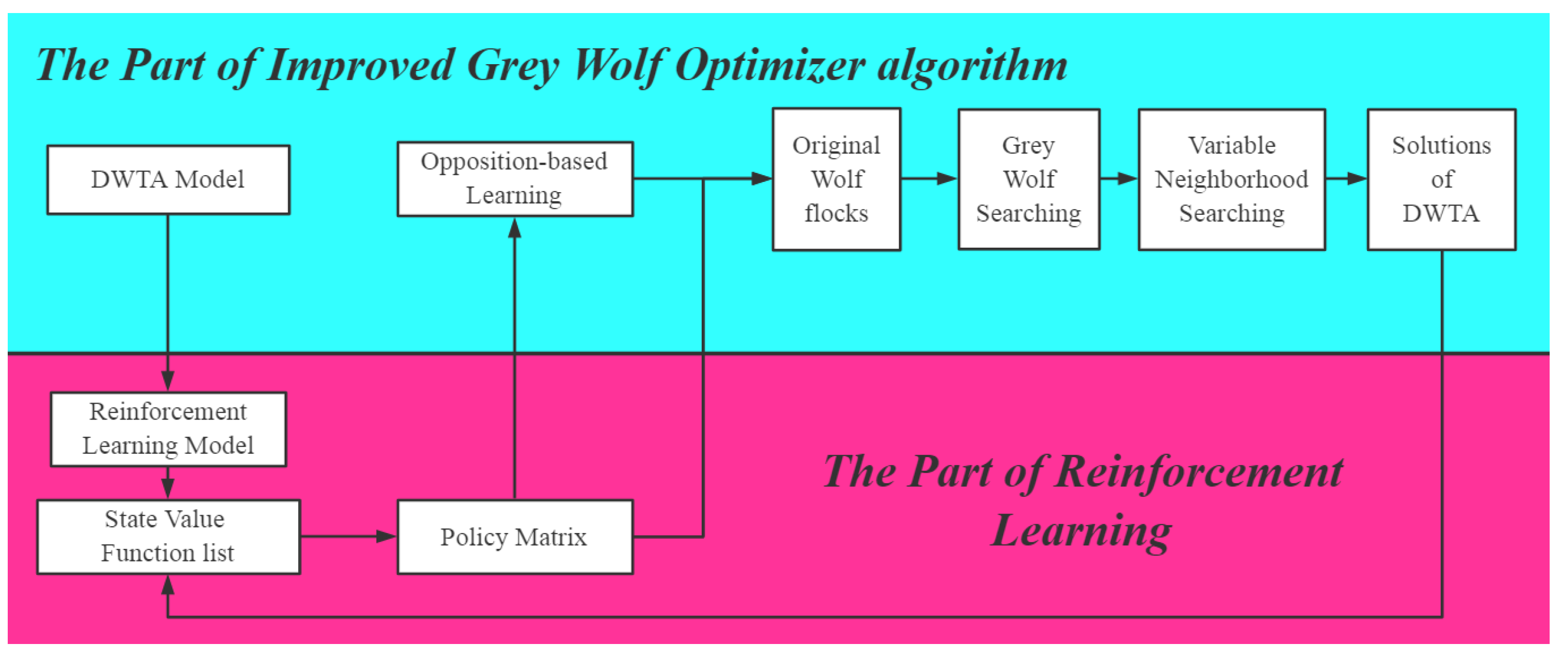
3. RL-IGWO Algorithm

3.1. DWTA Disassembly

The DWTA is a multi-stage sequential decision problem. In the weapon-target assignment in each stage, the variation of the battlefield situation needs to be considered in real time to obtain the global optimal solution in the time-domain.

Previous DWTA problems are mainly solved by using the framework of “Attack-Observation-Attack” (AOA), where “observation” refers to the analysis of the battlefield situation to determine the attack targets and available weapons, and “attack” refers to the determination of the WAT matrix, while the attack actions are implemented according to the decision. The process of “Observation-Attack” in the AOA framework is equated with a SWTA problem, and the DWTA problem is able to be equivalently expressed as several SWAT problems, as shown in the following Equation (18):

$$SWTA=\left\{{SWTA}^1,{SWTA}^2,\dots ,{SWTA}^{\mathrm{t}},\dots \right\}$$

(18)

where $t$ represents the $t-th$ stage of the $DWTA$, and $SWT{A}^t$ refers to the $SWTA$ of the $t-th$ stage of the $DWTA$.

The $SWT{A}^t$ of each stage t has its own objective function $J^t$, as shown in the following Equations (19) and (20):

$${SWT}^t=max J^t\left(A^t\right)$$

(19)

where $A^t$ represents the weapon-target assignment matrix in the $t-th$ stage of the $DWTA$.

$$J^t={{\displaystyle \sum }}_{i=1}^n{{\displaystyle \prod }}_{j=1}^n{(1-p_{ij}^t)}^{a_{ij}^t}$$

(20)

where $n$ indicates that there are n attacking targets in the $i-th$ stage of the$DWTA$; $i$represents the $i-th$ target; $m$ indicates that $m$ weapons can be used at this stage; $j$ refers to the $j-th$weapon; $p_{ij}^t$ represents the damage probability of weapon $j$ to target $i$ at the $t-th$ stage of the $DWTA$, which is determined by the traits of weapons; and $a_{ij}^t$ is the element of $A^t$ about row i and column j.

A DWTA problem is transformed into a multi-objective optimization problem through the framework work of “AOA”, as expressed in Equation (21), as follows:

$$DWTA=max \left\{J^1,J^2,\dots ,J^t,\dots \right\}$$

(21)

The strongest limitation of the AOA framework is that each $SWT{A}^t$ is only optimized in the local time-domain instead of the global time-domain. For example, in the frigate, at the first stage of defense against UAV swarms, the $SWT{A}^t$ generated by the OAO framework only considers the short-range air defense missile-1 at the current stage, without planning for the subsequent utilization of other weapons at the future stages. Although heuristic algorithms can solve static optimization problems well, DWTA is a typical sequential decision problem with strong randomness and traits sensitive to time. Once a decision is made, the decision cannot be changed, and the state transition caused by the action is uncertain, which renders difficulties in optimizing the multi-objective optimization problem of Equation (18) in the time-domain globally by means of a static heuristic method. Reinforcement learning is a method for solving sequential decision problems. As such, a model-based reinforcement learning framework was established [26,27,28], so as to transform DWTA problems into several SCO problems by means of the dynamic programming method.

According to the WTA matrix $A^t=[a_{ij}^t]$ and the damage probability matrix $P^t=[p_{ij}^t]$ at the$t-th$ stage, the expression of the number of damaged UAVs at the $t-th$ stage can be obtained, as shown in the following Equations (22) and (23):

$$death={{\displaystyle \sum }}_{i=1}^{n}broken\left(i\right)$$

(22)

$$broken\left(i\right)=\{\begin{array}{c}0,if x\le {\displaystyle {\displaystyle \prod }_{j=1}^4}{(1-p_{ij}^t)}^{a_{ij}^t}\\ 1,else\end{array}$$

(23)

where $broken\left(i\right)$ equals either 0 or 1, with 0 representing the successful penetration of the $i-th$ UAV, and 1 indicating the destruction of the $i-th$ UAV, while $x$ refers to a random number uniformly distributed from 0 to 1.

According to the multi-objective functions, the reward function of reinforcement learning is designed as shown in the following Equation (24):

$$r=\{\begin{array}{c}=-\infty ,if death<n and D=7\\ J_{ecr}\end{array}$$

(24)

Once a UAV breaks through the defense airspace, the frigate will pay an unacceptable price (a considerably large negative number), where w refers to an empirical parameter, representing the reward of each UAV being attacked, and the last four items represent the cost for damaging those UAVs. The purpose of such design is to reduce the cost-effectiveness ratio to the maximum extent under the constraints.

In this case, $n$ represents the number of UAVs at this state, and $S$, $D$ = 7 indicates that the UAV flock is within sub-area 7.

The state value function $v\left(S_t\right)$ of state $S$ at the $t-th$ stage is expressed by Equation (25). The value of the state value function $v\left(S_t\right)$ is stored in a 40 × 8 matrix $V_{40\times 8}$.

$$v\left(S_t\right)=E\left(r_t+r_{t+1}+r_{t+2}+r_{t+3}+\dots \right)$$

(25)

where $E( )$ represents the expectation function.

Assuming that the DWAT problem follows a Markov decision process and uses a greedy strategy when making decisions, the following Bellman discrete Equation (26) can be obtained for the state value function:

$$v_{k+1}\left(s_t\right)=max(r_{s_t}^A+{\displaystyle \sum }_{s_{t+1}}{P}_{s_t{s}_{t+1}}^A\times v\left(s_{t+1}\right))$$

(26)

where $v_k\left(s_t\right)$ represents the state value function of the $k-th$ iteration; $P_{s_t{s}_{t+1}}^A$ denotes the state transition probability matrix, representing the probability that state $s_t$ transitions to state $s_{t+1}$ under action $A$; and $r_{s_t}^A$ represents the reward value brought by the selection of action $A$ under state $s_t$. The state cost function is considered to converge as $v_k\left(s_t\right)$ approaches $v_{k+1}\left(s_t\right)$.

When the state value function converges, the DWTA problem is transformed into a series of static combination optimization (SCO) problems, as shown in the following Equations (27) and (28):

$$DWTA=\left\{SC{O}^1,SC{O}^2,\dots ,SC{O}^t,\dots \right\}$$

(27)

$$\{\begin{array}{c}SC{O}^t:max J\left(A^t\right)\\ J\left(A^t\right)=(r_{s_t}^A+{\displaystyle {\displaystyle \sum }_{s_{t+1}}}{P}_{s_t{s}_{t+1}}^A\times v\left(s_{t+1}\right))\end{array}$$

(28)

where $J\left(A^t\right)$ represents the objective function of this static combination optimization problem at the $t-th$ stage SCO(t).

3.2. Improved Grey Wolf Optimizer (IGWO)

The grey wolf optimizer (GWO) is a kind of new swarm intelligence optimization algorithm based on the social structures and predation behaviors of wolf packs. Through the verification of 29 standard optimization functions, the results of GWO were obviously superior to several traditional algorithms in solving accuracy and stability [29,30]. Grey wolf packs have a strict social hierarchy. The three wolves with the best performance are defined as leader wolves $\alpha$, $\beta$, and $\delta$, and the other wolves are defined as follower wolves. The follower wolves update their positions according to the condition of the leader wolves [31,32].

The original optimization process of GWO is shown in Algorithm 1.

Algorithm 1 Grey Wolf Optimizer

1: for $iter$ in range ($ite{r}_{\mathit{m}\mathit{a}\mathit{x}}$): 2:       for $i$ in range ($n$): 3:               $C_k=2\times random\left(0,1\right),k=1,2,3$ 4:               $D_{\alpha }=C_1{A}_{\alpha }-A_i\left(iter\right),D_{\beta }=C_2{A}_{\beta }-A_i\left(iter\right),D_{\delta }=C_3{A}_{\delta }-A_i\left(iter\right)$ 5:               $K_i=\left(2-iter/ite{r}_{\mathit{m}\mathit{a}\mathit{x}}\right)\times \left[2\times random\left(0,1\right)-1\right],k=1,2,3$ 6:               $A_1=A_{\alpha }-K_1{D}_{\alpha },A_2=A_{\beta }-K_2{D}_{\beta },A_3=A_{\delta }-K_3{D}_{\delta }$ 7:               $A_i\left(iter+1\right)=\left(A_1+A_2+A_3\right)/3$ 8:        end for 9: end for

In Algorithm 1, $A_{\alpha }$, $A_{\beta }$, and $A_{\delta }$ represent the positions of the leader wolves $\alpha$, $\beta$, and $\delta$; $A_i\left(iter\right)$ represents the position of the wolf-$i$ in the generation-$iter$; $D_{\alpha }$,$D_{\beta }$, and $D_{\delta }$ represent the search neighborhood generated by $\alpha$, $\beta$, and $\delta ; random\left(0,1\right)$ is a random number between (0,1), of which the randomness determines the uncertainty of the search neighborhood; $iter$ represents the generation of the wolf packs; $ite{r}_{max}$ represents the maximum generation; the parameter $K$ is a random number, of which the randomness determines the uncertainty of the searching direction and searching depth. If the absolute value of K is more than 1, the wolf packs will face towards the neighborhood to search. If the absolute value of K is less than 1, the wolf packs will face away from the neighborhood to search. The uncertainty of the search neighborhood evidently increases the global searching ability of the GWO.

In the present study, variable neighborhood search operators and an opposition-based learning operator were added to the GWO algorithm, which greatly enhanced the search ability in the global decision domain.

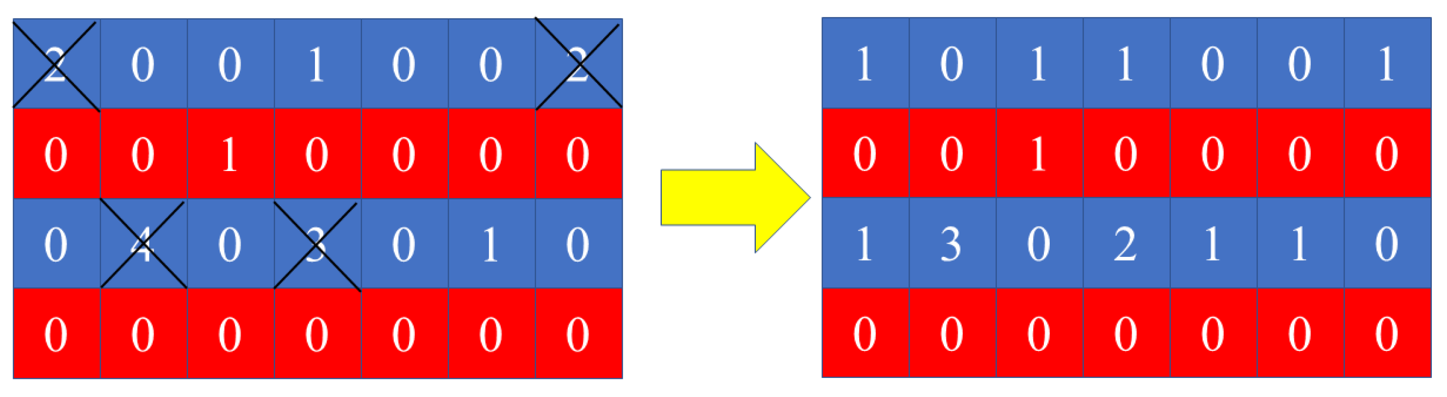
3.2.1. Opposition-based Learning Operator

Heuristic algorithms are mainly used to solve static optimization problems. Each optimization is an independent process, without the function of memory. For sequential decision optimization problems, the state value function of reinforcement learning makes up for the shortcomings of heuristic algorithms. A policy matrix $\pi$ was designed to store the position of leader wolves $\alpha ,\beta$, and $\delta$. Once the state value function is determined, the positions of leader wolves are conserved in the policy $\pi$, based on the experience gained by reinforcement learning.

In the process of operation, the three leader wolves are put into the initial wolf pack directly. The expression for matrix $\pi$ is shown in Equation (29), as follows:

$$\pi =\left[S,A_{\alpha },A_{\beta },A_{\delta }\right]$$

(29)

where $A_{\alpha },A_{\beta },and A_{\delta }$ represent the weapon-target assignment matrix of the leader wolves $\alpha ,\beta$, and $\delta$, respectively.

The initial position of wolves directly determines the convergence quality of optimization. In order to broaden the diversity of operations and avoid falling into the local optimal, a new opposition-based learning operator [33,34] was established for generating the initial position of wolves.

Leader wolves $\alpha$,$\beta$, and $\delta$ are selected, which are generated by the policy $\pi$ of reinforcement learning. Then, the opposition wolves $\widehat{\alpha }$,$\widehat{\beta }$, and $\widehat{\delta }$ are generated according to the leader wolves $\alpha$,$\beta$, and $\delta$. The process of opposition-based learning is shown as Figure 2.

The opposition-based position corresponds to the original position. The opposition-based operator will select the non-zero elements of the weapon-target assignment matrix A, and transform the elements equaling zero. The zero elements of matrix A will be transformed into non-zero randomly. The process of the opposition-based operator is described in Algorithm 2.

In Algorithm 2, $A_{\alpha }\left[ij\right]$ represents the weapon-target assignment matrix of the leader wolf,$A_{\widehat{\alpha }}\left[ij\right]$ represents the opposition-based weapon-target assignment matrix of the leader wolf, and $random.randint( )$ is a function for generating random integer numbers.

Algorithm 2 Opposition-Based Operator

1: Determine the position of leader wolfs: $A_{\alpha }\left[ij\right]$ 2:$B_{\alpha }\left[ij\right]$=$A_{\widehat{\alpha }}\left[ij\right]=A_{\alpha }\left[ij\right]$ 3:      for $i$ in range ($n1$): 4:           for $j$ in range ($n2$): 5:                if ($B_{\alpha }\left[ij\right]$ > 0): 6:                        $A_{\widehat{\alpha }}\left[ij\right]=0$ 7:                if ($B_{\alpha }\left[ij\right]$ = 0): 8:                        $A_{\widehat{\alpha }}\left[ij\right]=random.randint\left(0,3\right)$ 9:           end for 10:      end for 11: Output:$A_{\widehat{\alpha }}\left[ij\right]$

The illumination of OB operator is shown in Figure 3.

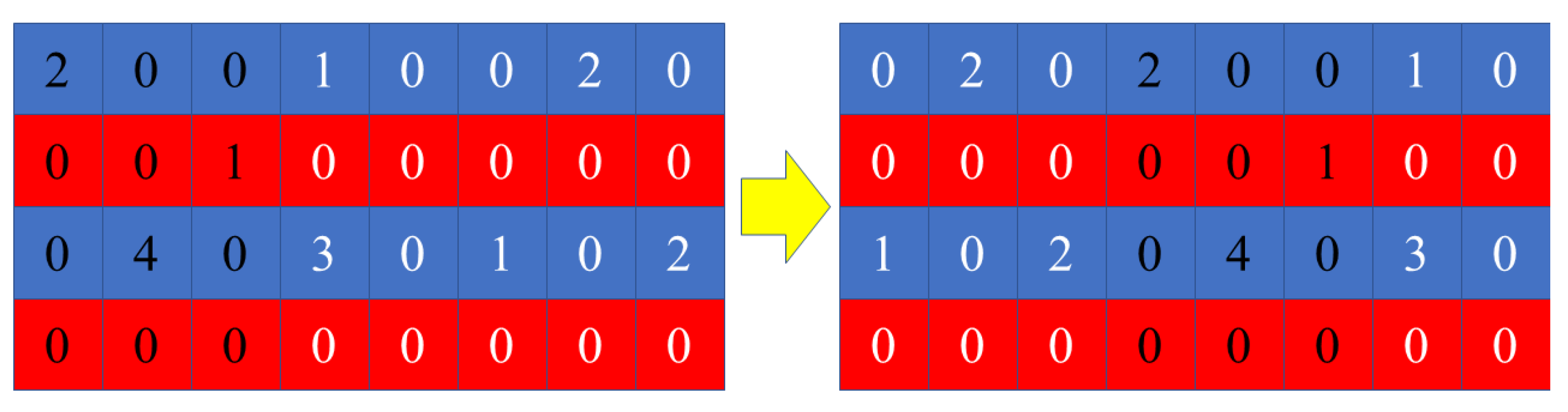
3.2.2. Variable Neighborhood Search Operator

In the present study, the variable neighborhood search method was adopted to enhance the local search ability of the grey wolf algorithm [35,36,37]. The algorithm flow is shown in Figure 4.

Three different variable neighborhood searching operators were designed, namely the balancing operator, sliding operator, and exploding operator. The wolves will find a superior solution based on the original solution, through transforming the searching neighborhood.

The balancing operator is designed to prevent over-concentration of resources about one target. The over-concentration of resources will increase the resource consumption of the defender. The process of the sliding operator is described in Algorithm 3.

In Algorithm 3, the parameter $\epsilon$ is a threshold of the resource concentration. The parameter $\epsilon$ can be settled from one to three. If the element of the weapon-target assignment matrix $A$ exceeds the threshold parameter $\epsilon$, the resource concentration part of corresponding elements will be reduced, and the reduced part will be assigned to the other elements randomly.

Algorithm 3 Balancing Operator

1: Determine the position of wolfs: $A\left[ij\right]$ 2: $B\left[ij\right]$=$A_B\left[ij\right]$=$A\left[ij\right]$ 3: for $i$ in range ($n1$): 4:      for $j$ in range ($n2$): 5:           if ($B\left[ij\right]$>$\epsilon$): 6:                     $A_B\left[ij\right]=B\left[ij\right]-1$ 7:                       Select k satisfies ($B\left[ik\right]$<$\epsilon$) 8:                      $A_B\left[ik\right]=B\left[ik\right]+1$ 9:          end for 10: end for 11: Output: $A_B\left[ij\right]$

The illumination of the balancing operator is shown in Figure 5.

The sliding operator was designed to construct a new neighborhood. The process of the sliding operator is described in Algorithm 4.

Algorithm 4 Sliding Operator

1: Determine the position of wolves: $A\left[ij\right]$ 2: $n$ = 3, $t$ = 1 3: $B\left[ij\right]$=$A_s\left[ij\right]$=$A\left[ij\right]$ 4: $A_s\left[i,n2\right]$=$B\left[i,0\right]$,$A_s\left[i,n2-1\right]$=$B\left[i,1\right]$,$A_s\left[i,n2-2\right]$=$B\left[i,2\right]$ 5: for $i$ in range ($n1$): 6:          for $j$ in range (0,$n2-3$): 7:                   $A_s\left[i,j\right]$=$B\left[i,j+3\right]$ 8:          end for 9: end for 10: Output:$A_s\left[i,j\right]$

In Algorithm 4, the sliding operator creates a new neighborhood by means of the sliding method. The parameter $n$ determines the sliding units in the process of the sliding operator. The parameter $t$ is a random integer from one to three, which will determine the operation of each clown. When the parameter $t$ is zero, the relevant elements of the weapon-target assignment matrix will stay in the original position. When the parameter $t$ is one, the relevant elements of the weapon-target assignment matrix will slide $n$ units left. When the parameter $t$ is minus one, the relevant elements of the weapon-target assignment matrix will slide $n$ units right. The illumination of the sliding operator is shown in Figure 6.

When the balancing operator and sliding operator are not able to generate superior solutions, the exploding operator is adopted. The exploding operator will generate a random sequence, forming a new weapon-target assignment matrix. Although the exploding operator will explore massive feasible solutions and improve the global searching ability, the original structure of the neighborhood will also be destroyed, and the excellence of the initial solution will be missed. Attempts were made to maintain a balance between local and global search, while maintaining diversity. The process of the balancing operator is as shown in the following Equations (30)–(35):

$$A_i^{exploding}=X_i+E_i$$

(30)

where $A_i$ is the original solution$, E_i$ is the exploding part, and $A_i^{exploding}$ is the solution generated by the exploding operator.

The expression of the exploding part $E_i$ is shown in Equation (29), as follows:

$$E_i={\widehat{E}}_i+{\tilde{E}}_i$$

(31)

where ${\tilde{E}}_i$ is stochastic disturbance term of $E_i$, and ${\widehat{E}}_i$ is the neighbors learning term of $E_i$.

The expression of the stochastic disturbance term ${\tilde{E}}_i$ is shown in Equation (30), as follows:

$${\tilde{E}}_i\left[I,J\right]=E_{max}\times \left(1-iter/ite{r}_{max}\right)·\delta$$

(32)

where $\delta$ is a random number from −1 to 1,$E_{max}$ is the maximum scope of the stochastic disturbance$; {\tilde{E}}_i\left[I,J\right]$ is the element of row $I$ and column $J$ of the matrix ${\tilde{E}}_i$.

The expression of the neighbors learning term ${\widehat{E}}_i$ is as shown in the following Equation (31):

$${\widehat{E}}_i={\displaystyle {{\displaystyle \sum }}_{A_j\in N_i}}\left(A_j-A_i\right)$$

(33)

where $N_i$ is a neighborhood of the solution $A_i$.

The expression of the neighborhood of the solution $A_i$ is shown in Equation (32), as follows:

$$N_i=\{A_j|(\Vert A_j-A_i\Vert <R_i)\}$$

(34)

where $R_i$ is the neighborhood radius of $N_i$, and$A_j-A_i$ is the distance between $A_i$ and $A_j$.

The expression of the neighborhood radius $R_i$ is shown in Equation (33), as follows:

$$R_i=\frac{1}{5n}{{\displaystyle \sum }}_{j=1}^n\Vert A_i-A_j\Vert$$

(35)

where $n$ is the number of the wolf population.

3.3. Flow of Improved Grey Wolf Optimizer Based on Reinforcement Learning (RL-IGWO)

The flow of RL-IGWO is shown in Figure 7.

The DWTA model was established from the scenario of a frigate defending against UAV swarms. The constraints of the model of DWTA were extracted from the real constraint conditions of a frigate’s anti-air system. The multi-objective functions were designed according to the evaluation indicators of the battlefield, such as destruction value$(D_v)$, resource consumption$(R_c)$, efficiency-cost ratio$(E_{cr})$, average interception rate$\left(A_{ir}\right)$, and defense completion rate$(D_{cr})$.

Based on the damage probability of the anti-air weapon system of the frigate, the state transition probability matrix was known, and the reinforcement learning based on model was able to be directly established. The state value function of reinforcement learning generated the initial generation of the grey wolf pack. The experience accumulated by reinforcement learning improved the GWO’s searching ability.

The reinforcement learning framework can transform a DWTA problem into a series of SCO problems, which enables the grey wolf algorithm to search for global optimal solutions in the time-domain. The improved grey wolf algorithm also helps the state value function converge rapidly.

4. Numerical Experiment

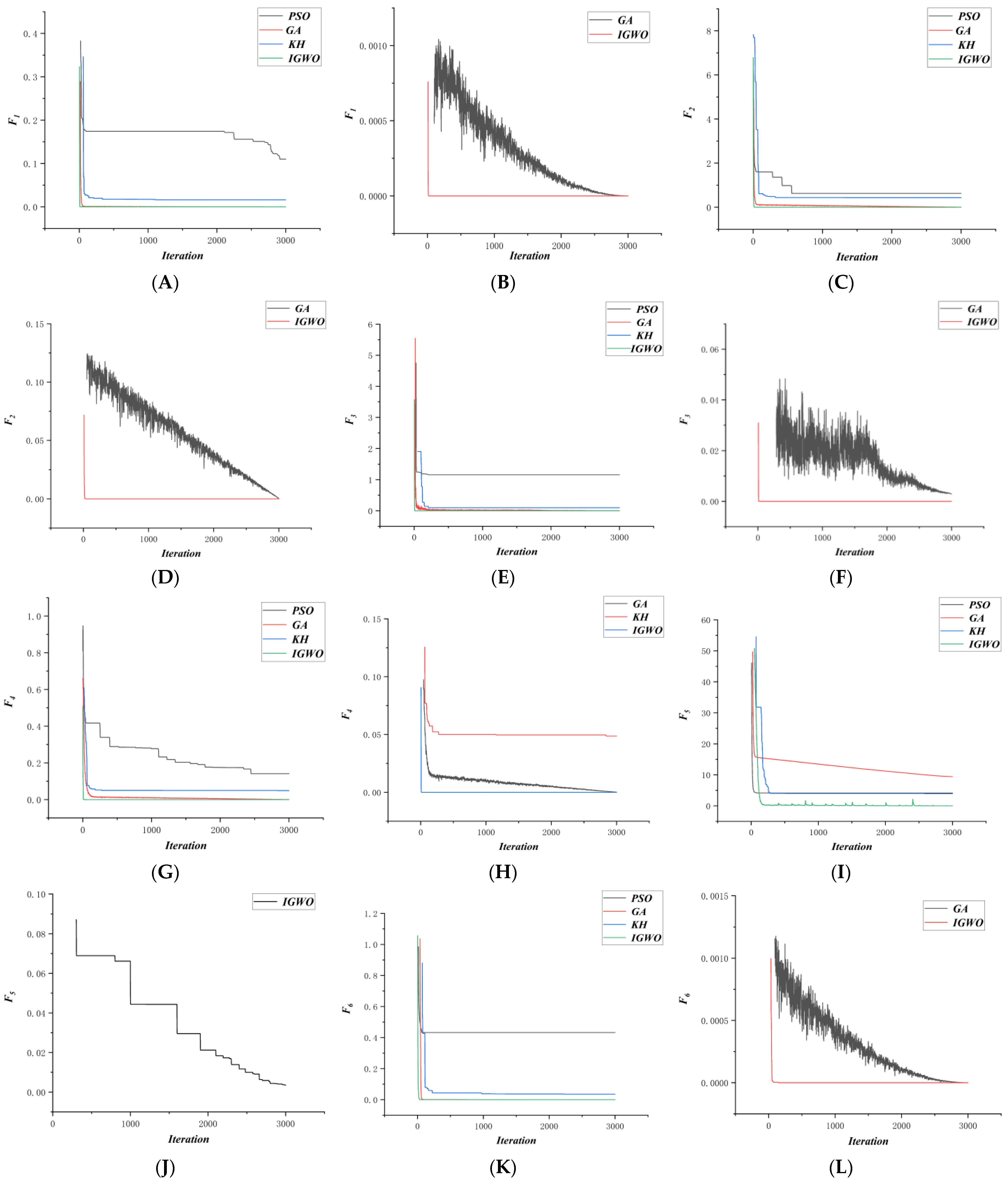
4.1. Simulation of Benchmark Functions

The performance evaluation of the I-GWO was conducted by means of the CEC benchmark suite [38,39], and six unimodal test functions were selected, as shown in

Table 4. Benchmark functions.

Name	Benchmark Function	Dimension	Variable Bounds	Theoretical Value
F1	$f_1\left(x\right)={\displaystyle \sum }_{i=1}^n{x}_i^2$	20	[−100,100]	0
F2	$f_2\left(x\right)={\displaystyle \sum }_{i=1}^n\left|x_i\right|+{\displaystyle \prod }_{i=1}^n\left|x_i\right|$	20	[−100,100]	0
F3	$f_3\left(x\right)={\displaystyle \sum }_{i=1}^n[{({\displaystyle \sum }_{j=1}^i{x}_j)]}^2$	20	[−100,100]	0
F4	$f_4\left(x\right)=max\left\{\left|x_i\right|,1\le i\le n\right\}$	20	[−100,100]	0
F5	$f_5\left(x\right)={\displaystyle \sum }_{i=1}^{n-1}[100{\left(x_{i+1}-x_i^2\right)}^2+{\left(x_i-1\right)}^2]$	20	[−30,30]	0
F6	$f_6\left(x\right)={\displaystyle \sum }_{i=1}^n{\left[\left(x_i+0.5\right)\right]}^2$	20	[−100,100]	0

. All benchmark functions were evaluated with dimension of 20 by 20 independent runs.

All the experiments were implemented using Python 3.8.5 and run on a desktop with 1.8 GHz Core i7-8565U CPU and 16.00 GB RAM.

The results of the I-GWO were compared with the state-of-the-art metaheuristic algorithms, namely particle swarm optimization (PSO) [40], krill herd algorithm (KH) [41] and genetic algorithm (GA) [42]. As shown in

Table 5. Parameters of algorithms.

Algorithm	Population Size	Iteration
PSO	1500	3000
GA	1500	3000
KH	50	3000
IGWO	50	3000

, in all experiments, the parameters of the comparative algorithms were the same as the recommended settings.

The optimization results of the different algorithms on the benchmark functions are shown in

Table 6. Results of benchmark functions.

Test Problems	Statistic	PSO	GA	KH	IGWO
F1	max	$0.50\times {10}^{-1}$	$1.74\times {10}^{-8}$	$4.21\times {10}^{-2}$	$0$
	min	$2.23\times {10}^{-2}$	$8.55\times {10}^{-9}$	$1.32\times {10}^{-2}$	$0$
	ave	$2.86\times {10}^{-1}$	$1.44\times {10}^{-8}$	$2.49\times {10}^{-2}$	$0$
	std	$2.05\times {10}^{-2}$	$4.51\times {10}^{-9}$	$1.07\times {10}^{-2}$	$0$
F2	max	$3.08\times {10}^0$	$4.63\times {10}^{-4}$	$7.20\times {10}^{-1}$	$0$
	min	$6.26\times {10}^{-1}$	$3.71\times {10}^{-4}$	$4.35\times {10}^{-1}$	$0$
	ave	$1.56\times {10}^0$	$4.15\times {10}^{-4}$	$5.92\times {10}^{-1}$	$0$
	std	$9.61\times {10}^{-1}$	$3.22\times {10}^{-5}$	$1.07\times {10}^{-1}$	$0$
F3	max	$9.26\times {10}^0$	$8.92\times {10}^{-3}$	$7.64\times {10}^{-1}$	$0$
	min	$1.16\times {10}^0$	$2.90\times {10}^{-3}$	$9.77\times {10}^{-2}$	$0$
	ave	$3.74\times {10}^0$	$6.33\times {10}^{-3}$	$3.46\times {10}^{-1}$	$0$
	std	$3.09\times {10}^0$	$2.38\times {10}^{-3}$	$2.65\times {10}^{-1}$	$0$
F4	max	$3.47\times {10}^{-1}$	$1.15\times {10}^{-4}$	$6.40\times {10}^{-2}$	$0$
	min	$1.41\times {10}^{-1}$	$1.06\times {10}^{-4}$	$4.86\times {10}^{-2}$	$0$
	ave	$2.52\times {10}^{-1}$	$1.12\times {10}^{-4}$	$5.56\times {10}^{-2}$	$0$
	std	$7.92\times {10}^{-2}$	$1.43\times {10}^{-5}$	$6.88\times {10}^{-3}$	$0$
F5	max	$1.84\times {10}^1$	$1.02\times {10}^1$	$2.53\times {10}^1$	$6.11\times {10}^0$
	min	$1.25\times {10}^0$	$9.44\times {10}^0$	$3.92\times {10}^0$	$3.56\times {10}^{-3}$
	ave	$7.54\times {10}^0$	$9.78\times {10}^0$	$1.07\times {10}^1$	$3.26\times {10}^0$
	std	$6.17\times {10}^0$	$4.47\times {10}^{-1}$	$7.78\times {10}^0$	$3.71\times {10}^0$
F6	max	$8.75\times {10}^{-1}$	$2.39\times {10}^{-8}$	$6.97\times {10}^{-2}$	$9.05\times {10}^{-9}$
	min	$4.32\times {10}^{-1}$	$1.58\times {10}^{-8}$	$3.57\times {10}^{-2}$	$3.32\times {10}^{-11}$
	ave	$6.31\times {10}^{-1}$	$2.09\times {10}^{-8}$	$5.05\times {10}^{-2}$	$4.61\times {10}^{-9}$
	std	$1.71\times {10}^{-1}$	$4.25\times {10}^{-9}$	$1.59\times {10}^{-2}$	$3.69\times {10}^{-9}$

.

Table 6 shows the optimization results of the different algorithms on the benchmark functions. For the benchmark functions F1 to F4, the IGWO algorithm was able to converge to the theoretical minimum value, while the PSO algorithm, the KH algorithm, and the GA algorithm had problems of local convergence in different degrees for high-dimensional problems. Among said algorithms, the results of the GA genetic algorithm were better than the KH algorithm, and the KH algorithm was better than the PSO algorithm. For the benchmark function F5, all algorithms fell into local convergence in different levels within 3000 iterations. Among the algorithms, the optimal value of the IGWO algorithm was three orders of magnitude higher than the other three algorithms, and the optimization results of the PSO algorithm was significantly superior to the GA algorithm and the KH algorithm. For the benchmark function F6, the IGWO algorithm and the GA algorithm were superior to the KH algorithm and the PSO algorithm in global searching ability. The results of the IGWO algorithm were one order of magnitude higher than the GA algorithms, and the local convergence phenomenon of the PSO algorithm was the most significant.

The best optimization processes of different algorithms in benchmark functions are shown in Figure 8.

Figure 8 shows the optimization process of the different algorithms on the benchmark functions. For the benchmark functions F1 to F4, the IGWO algorithm converged to the theoretical value rapidly in finite iterations, and the PSO algorithm and the KH algorithm fell into local convergence for high-dimensional problems. The GA algorithm, although exhibiting serious oscillation, still exhibited a strong global search ability, constantly approaching the theoretical minimum value, albeit at a considerably slower rate of convergence than IGWO. For the benchmark function F5, the genetic algorithm performed poorly, failing to converge within 3000 iterations. The PSO and KH algorithms optimized rapidly in the initial phase and then fell into local convergence. The IGWO algorithm approached the theoretical minimum after several oscillations in the process of global optimization-seeking.

For the benchmark function F6, the PSO algorithm converged rapidly and then fell into a local optimal immediately. Although the KH algorithm successfully left a local convergence state several times, the algorithm still fell back into local convergence eventually. Further, the results of the KH algorithm were already substantially superior to those of the PSO algorithm. The results of both the GA algorithm and the IGWO algorithm were close to the theoretical minimum value; however, the GA algorithm was significantly slower than the IGWO algorithm in terms of optimization speed.

To enhance the search ability of the grey wolf optimizer algorithm, the methods of opposition-based learning operator and variable neighbor search operator were adopted. The experiments on the benchmark functions demonstrate that the IGWO algorithm was superior to several state-of-the-art metaheuristic algorithms.

4.2. Numerical Experiment of DWTA Problems

4.2.1. Parameters of Numerical Experiment

In the numerical experiment, six different battle scenarios were simulated, each of which was repeated 35 times to test the algorithm performance in different population scales and iterating generations. Through simulation results and algorithm comparison, the advantages of the RL-IGWO algorithm could be identified in terms of decision making time and solution quality.

At present, there is no single performance indicator that can comprehensively measure the performance of an algorithm in respect to DWTA problems. Therefore, several typical indicators were selected to compare the performance of different algorithms, such as destruction value$(D_v)$, resource consumption$(R_c)$, efficiency-cost ratio$(E_{cr})$, average interception rate$\left(A_{ir}\right)$, and defense completion rate$(D_{cr})$.

For all algorithms, the public parameters were first set as shown in

Table 7. Parameters of algorithms.

Scenario		Scen1	Scen2	Scen3	Scen4	Scen5	Scen6
Pop	RL-IGWO	10	10	10	10	50	50
	Others	10	10	50	50	50	50
Gen		20	100	20	50	20	50

, with Pop representing the population size, and Gen representing the number of iterations.

Table 8. Parameters of scenarios.

Parameters	Scen1	Scen2	Scen3	Scen4	Scen5	Scen6
Number	40	39	38	37	36	35
Region	D1	D1	D2	D2	D3	D3

shows the relevant parameters of each scenario. Number represents the number of the surviving UAV swarms, while Region represents the sub-area where the UAV swarms exist.

4.2.2. Process of Reinforcement Learning

In the present study, a model-based reinforcement learning framework was established according to the scenario of a frigate defending against UAV swarms, so as to train a weapon-target assignment policy. Policy evaluation and policy iterations are the major parts of the process of reinforcement learning, and these two steps are executed alternately until the optimal strategy is obtained.

The validity of the aforementioned theorem is based on the greedy extent of the greedy strategy. The greedy extent of the greedy strategy directly determines the convergence speed and convergence quality of the state value function. In the present study, the original grey wolf optimizer (GWO) algorithm and the improved grey wolf optimizer (IGWO) algorithm were used to search for the optimal actions in decision space, executing the greedy strategy. The convergence of the state value under different policies is shown in Figure 9. The horizontal axis is the number of iterations, and the vertical axis is the state value. Graph (A) corresponds to the state (40,0); Graph (B) corresponds to the state (35,0); Graph (C) corresponds to the state (30,1); Graph (D) corresponds to the state (20,2); Graph (E) corresponds to the state (10,3); and Graph (F) corresponds to the state (5,4). The black line represents the state value function of the improved grey wolf optimizer (IGWO) algorithm, and the red line represents the state value function of the original grey wolf optimizer (GWO) algorithm.

Through the results of policy evaluation, the improved grey wolf optimizer algorithm (IGWO) obviously had higher global searching ability than the original grey wolf optimizer algorithm (GWO). State (5,4) and state (10,3) were close to the ultimate state. Because the state value of the ultimate state was directly set as a large negative number, the state values of state (5,4) and state (10,3) were determined by the ultimate state to a large extent. Hence, the results of IGWO were slightly better than those of GWO, but the convergence speed of IGWO was still significantly higher than GWO.

State (40,0), state (35,0), state (30,1), and state (20,3) were far away from the ultimate state. The state value functions were determined by the policy to a large extent. The policy evaluation results show that the policy based on IGWO had a higher state value than the policy based on GWO. The policy based on IGWO also had advantages in convergence speed.

For state (40,0), the results of policy based on GWO even exhibited a slight oscillation phenomenon, without convergence. For state (40,0), the state value of policy based on IGWO was almost three times as high as the policy based on GWO. As such, the effectiveness of the IGWO algorithm in terms of DWAT problems has been adequately demonstrated.

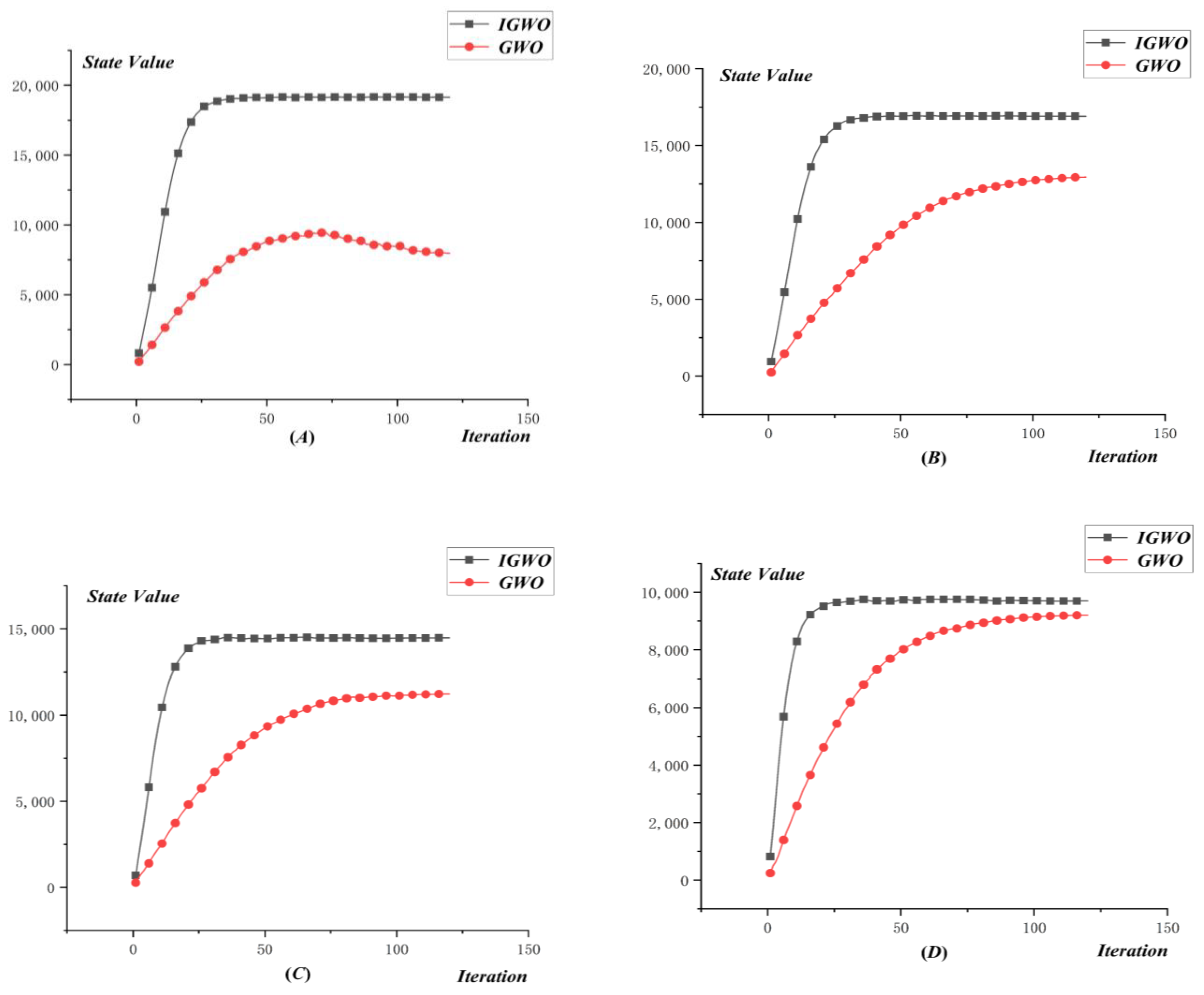
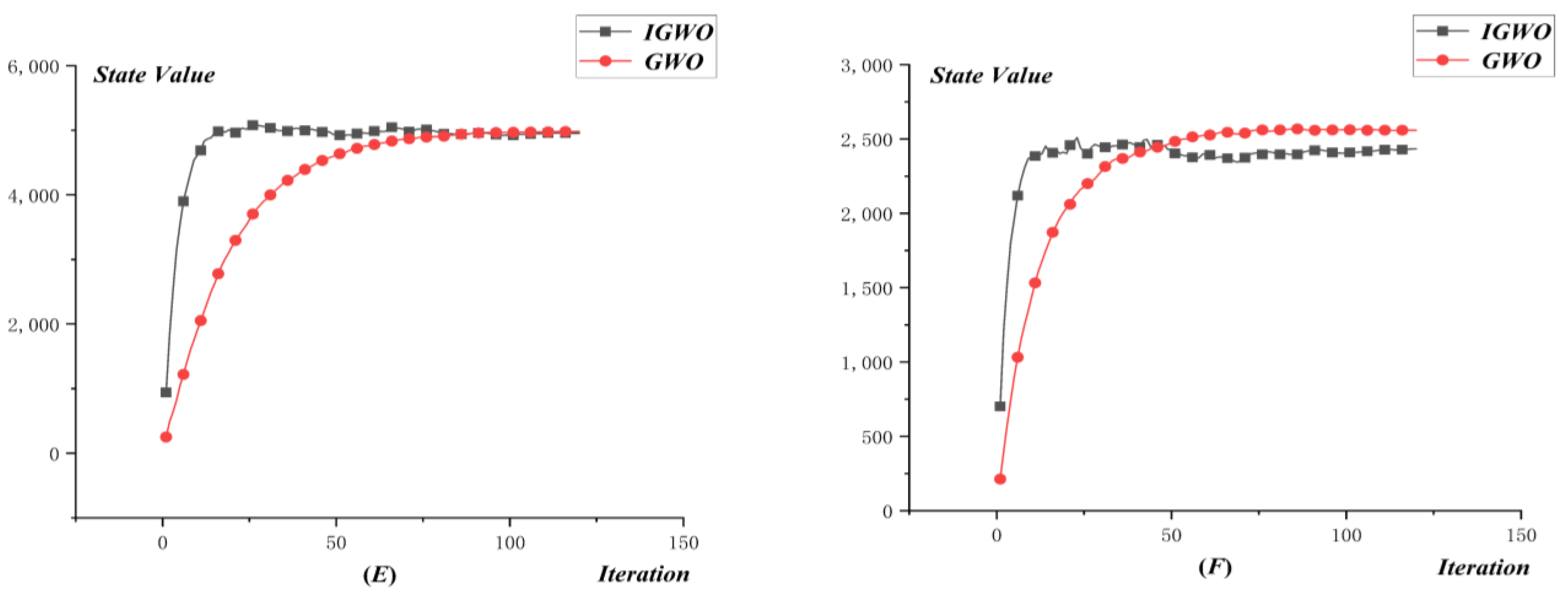
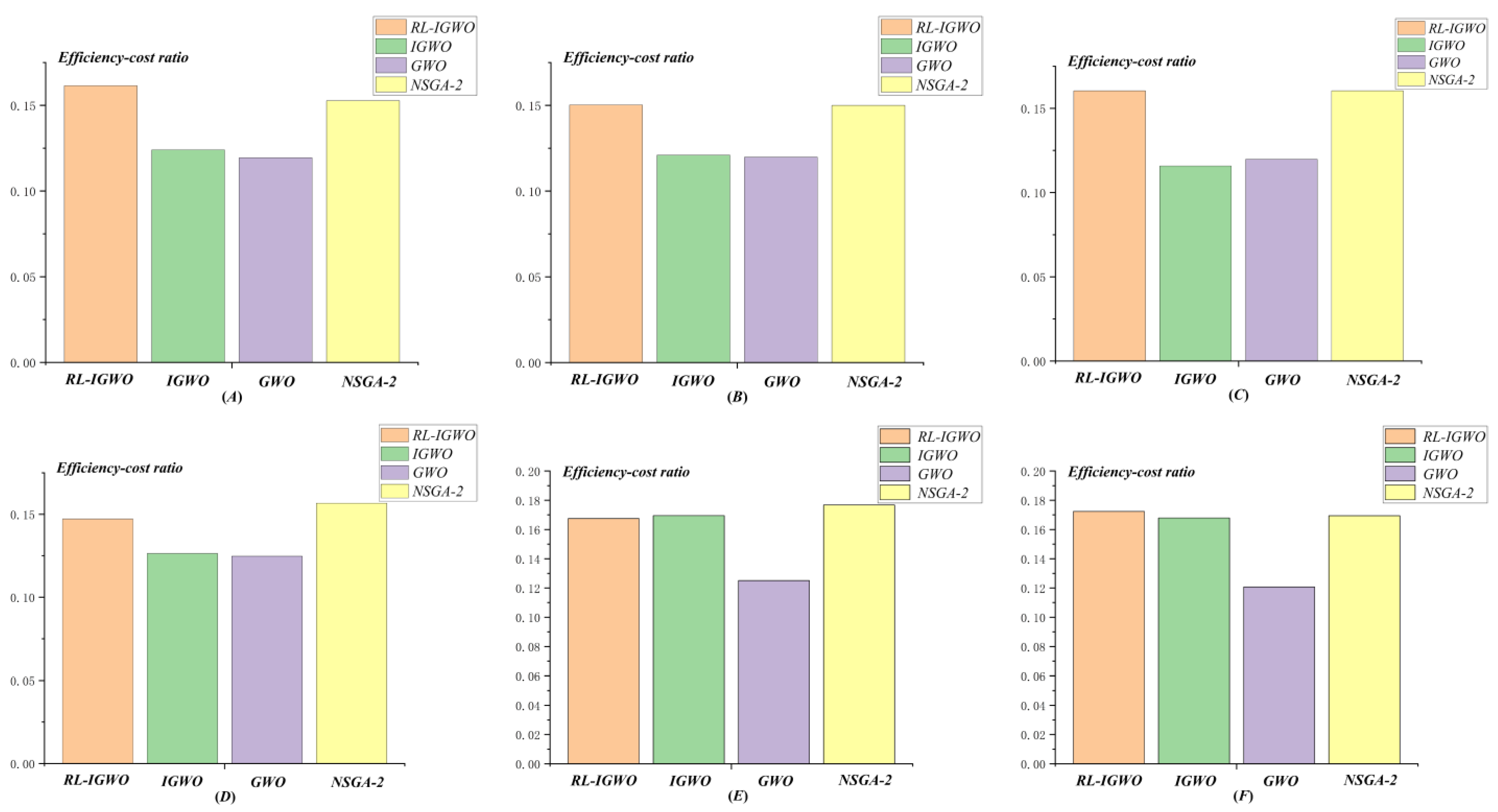
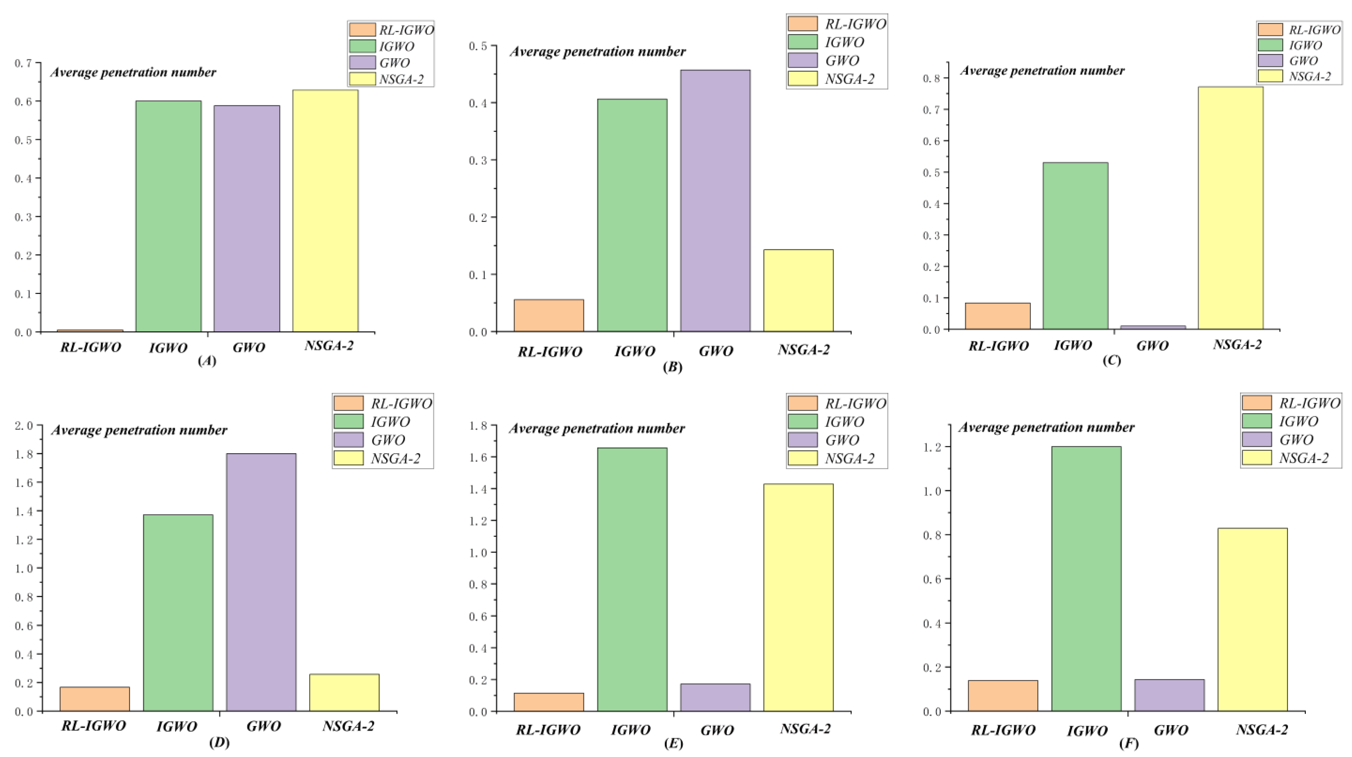
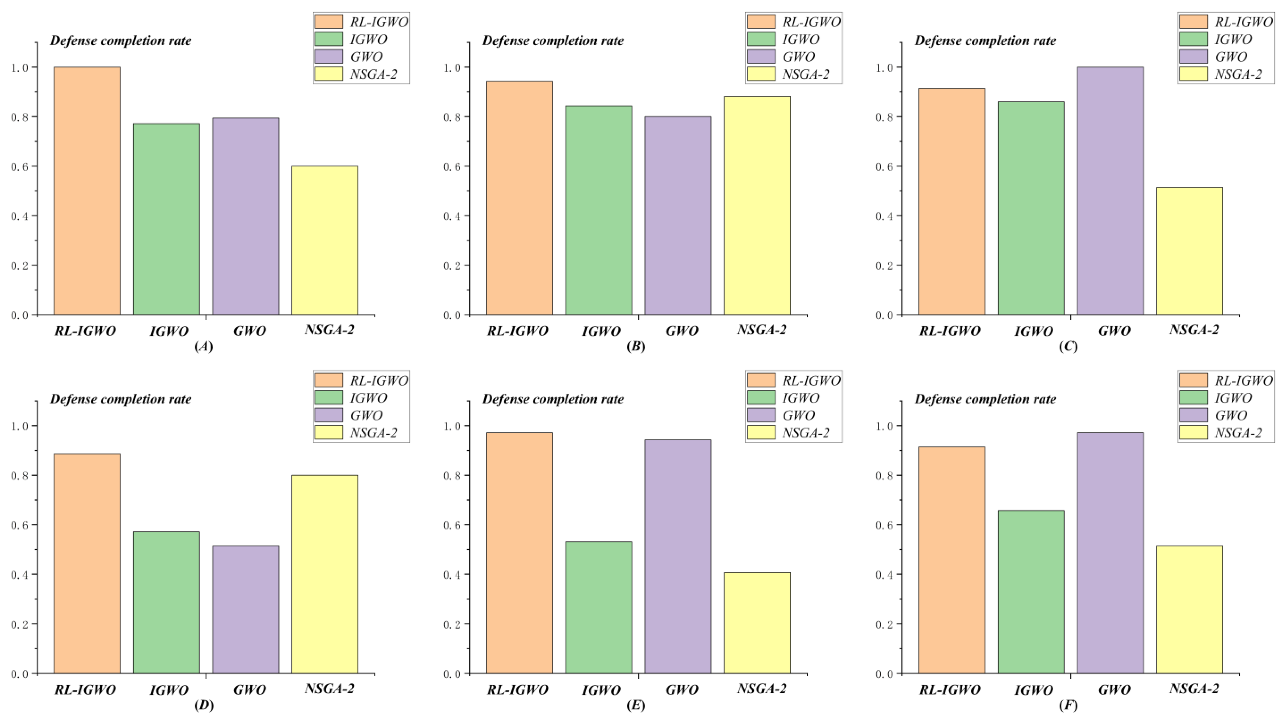
4.2.3. Results of DWTA

In order to prove the effectiveness of the improved grey wolf optimizer algorithm based on reinforcement learning (RL-IGWO), the algorithm was compared with three other algorithms, including original grey wolf optimizer algorithm (GWO), the improved grey wolf optimizer algorithm (IGWO), and the multi-objective nondominated sorting genetic algorithm (NSGA-2), where the unified crossover and random mutation operators were applied.

The simulation results of different indicators, namely destruction value $(D_v)$, resource consumption$(R_c)$, efficiency-cost ratio$(E_{cr})$, average interception rate$\left(A_{ir}\right)$, and defense completion rate$(D_{cr})$ under four different algorithms were as follows. The comparison of the destruction values is shown in

Table 9. Comparison of destruction values.

Scenario	${\mathit{D}}_{\mathit{v}}$	RL-IGWO	IGWO	GWO	NSGA-2
Scen1	Average	800	788.0	788.2	787.4
	Std. dev	0	27.1	26.2	19.2
	Median	800	800.0	800.0	800.0
	Maximum	800	800.0	800.0	800.0
	Minimum	800	680.0	700.0	720.0
Scen2	Average	778.9	771.9	770.9	777.1
	Std. dev	4.6	22.8	21.0	8.5
	Median	780.0	780.0	780.0	780.0
	Maximum	780.0	780.0	780.0	780.0
	Minimum	760.0	680.0	700.0	740.0
Scen3	Average	758.3	760	760.0	744.6
	Std. dev	5.6	0.0	0.0	18.6
	Median	760.0	760	760.0	760.0
	Maximum	760.0	760	760.0	760.0
	Minimum	740.0	760	760.0	700.0
Scen4	Average	736.6	712.6	704.0	734.9
	Std. dev	11.2	38.9	44.5	12.0
	Median	740.0	740.0	740.0	740.0
	Maximum	740.0	740.0	740.0	740.0
	Minimum	680.0	600.0	600.0	680.0
Scen5	Average	717.7	686.9	716.6	692.5
	Std. dev	13.3	39.2	14.7	27.7
	Median	720.0	720.0	720.0	700.0
	Maximum	720.0	720.0	720.0	720.0
	Minimum	640.0	580.0	640.0	640.0
Scen6	Average	697.1	676.0	697.1	683.4
	Std. dev	10.8	39.9	16.7	20.6
	Median	700.0	700.0	700.0	700.0
	Maximum	700.0	700.0	700.0	700.0
	Minimum	640.0	580.0	600.0	620.0

.

Based on the results of Table 9, the UAV swarm destruction values under the weapon-target assignment policy based on RL-IGWO were obviously higher than the GWO, IGWO, and NSGA-2 algorithms. The average value and median value of the UAV swarm destruction values under RL-IGWO were also higher than the GWO, IGWO, and NSGA-2 algorithms. For Scen1 and Scen2, the results of RL-IGWO were superior to the other algorithms. The results of GWO and IGWO were similar, being higher than NSGA-2, but the results of NSGA-2 were more stable than GWO and IGWO. For Scen3 and Scen4, the RL-IGWO algorithm, with a smaller population and fewer iterations, obtained better solutions than the other algorithms, which demonstrates that the proposed RL-IGWO had stronger goal searching ability. For Scen3, the results of IGWO were superior to GWO, and the NSGA-2 performed poorly. Comparing “Scen1 and Scen2” with “Scen5 and Scen6”, the RL-IGWO algorithm could offer dynamic weapon-target assignments of high destruction values in different air-defense regions.

The comparison of resource consumption is shown in

Table 10. Comparison of resource consumption.

Scenario	${\mathit{R}}_{\mathit{c}}$	RL-IGWO	IGWO	GWO	NSGA-2
Scen1	Average	4953.3	6353.9	6600.6	5156.4
	Std. dev	444.0	1580.8	706.8	236.3
	Median	4946.0	5786.0	6510.5	5176.0
	Maximum	5980.0	11,824.0	7997.0	5502.0
	Minimum	4212.0	4798.0	5274	4576.0
Scen2	Average	5182.5	6378.6	6432.4	5179.2
	Std. dev	401.2	1147.0	838.4	175.9
	Median	5178.0	6187.5	6352.0	5199.0
	Maximum	6124.0	9993.0	9478.0	5506.0
	Minimum	4450.0	5007.0	5368.0	4721.0
Scen3	Average	4727.7	6562.5	6344.8	4640.8
	Std. dev	484.6	985.8	638.2	220.2
	Median	4677.0	6239.5	6263.0	4636.0
	Maximum	6357.0	8791.0	8009.0	5179.0
	Minimum	3965.0	5060.0	5031.0	4212.0
Scen4	Average	5005.4	5636.4	5642.0	4688.6
	Std. dev	446.9	2081.9	607.3	227.1
	Median	4989.0	5202.0	5446.0	4697.0
	Maximum	6333.0	14,450.0	6761.0	5156.0
	Minimum	4000.0	4183.0	4276.0	4209.0
Scen5	Average	4285.3	4051.8	5726.6	3916.5
	Std. dev	383.6	498.5	688.2	214.7
	Median	4310.0	3993.5	5756.0	3888.0
	Maximum	5127.0	5269.0	7081.0	4303.0
	Minimum	3665.0	3125.0	4226.0	3485.0
Scen6	Average	4043.9	4025.4	5773.2	4033.6
	Std. dev	354.7	1225.5	562.0	289.8
	Median	4072.0	3751.0	5731.0	4087.0
	Maximum	4730.0	10778.0	7161.0	4485.0
	Minimum	3200.0	3253.0	4742.0	3361.0

.

Based on the results of Table 10, the UAV swarm resource consumption under the weapon-target assignment policy based on RL-IGWO was lower than the IGWO and GWO algorithms. The standard deviation of RL-IGWO was at a low level, showing that the results under RL-IGWO were more stable than the GWO and IGWO algorithms. The resource consumption of NSGA-2 was slightly better than RL-IGWO, but NSGA-2 performed poorly in terms of average interception rate$\left(A_{ir}\right)$, and defense completion rate$(D_{cr})$. For Scen1 and Scen2, the results of RL-IGWO were significantly lower than GWO and IGWO, and at the same level as the results of NSGA-2. For Scen3 and Scen4, the RL-IGWO algorithm, with a lower population and fewer iterations, was able to obtain a better solution with lower resource consumption. Comparing “Scen1 and Scen2” with “Scen5 and Scen6”, the RL-IGWO algorithm could offer dynamic weapon-target assignments of low resource consumption in different air-defense regions. For Scen5 and Scen6, the operational research ability of the IGWO algorithm was much higher than that of the GWO algorithm, being at the same level as the results of RL-IGWO.

The results of efficiency-cost ration $(E_{cr})$, average interception rate $\left(A_{ir}\right)$, and defense completion rate $(D_{cr})$ under different algorithms are shown in Figure 10, Figure 11 and Figure 12. Graph(A) to Graph(F) correspond to the Scen1 to Scen6 in Figure 10, Figure 11 and Figure 12. The orange bar chart is the results under the policy based on the RL-IGWO algorithm. The green bar chart is the results under the policy based on the IGWO algorithm. The purple bar chart is the results under the policy based on the GWO algorithm. The yellow bar chart is the results under the policy based on the NSGA-2 algorithm.

Based on the results of Figure 10, the efficiency-cost ratio based on the RL-IGWO was much higher than the IGWO and GWO algorithms, at the same level as the results of NSGA-2. The efficiency-cost ratio of IGWO was slightly higher than that of GWO. For Scen1, Scen2, Scen3, and Scen4, the efficiency-cost ratio of the RL-IGWO algorithm exhibited a slight decrease to some extent, with the number of iterations increasing. As the number of iterations increases, the superiority of the initial population provided by the reinforcement learning strategy is likely to gradually disappear, and, thus, the local search operators of IGWO should maintain a balance between exploration and exploitation. For Scen3 and Scen4, the RL-IGWO algorithm, with a smaller population and fewer iterations, was able to obtain a better solution with higher efficiency-cost ratio. Comparing “Scen1 and Scen2” with “Scen5 and Scen6”, the RL-IGWO algorithm could offer dynamic weapon-target assignments of high efficiency-cost ratio in different air-defense regions.

Based on the results of Figure 11, the average penetration number based on RL-IGWO was significantly superior to the IGWO, GWO, and NSGA-2 algorithms, with NSGA-2 being the worst. For Scen2, Scen5, and Scen6, the average penetration number of the IGWO algorithm was even higher than that of the GWO algorithm. However, IGWO had a stronger optimization capability than GWO, which also could not guarantee a better weapon-target assignment scheme. On the premise of defending against UAV swarms successfully, the efficiency-cost ratio was enhanced greatly, which is the fundamental interest of frigates. In fact, higher requirements are established for model construction, and objective functions need to achieve a reasonable balance under a variety of conflicting indicators. For the RL-IGWO algorithm, attempts were made to solve the conflict of different indicators by designing a new objective function, in which value state functions of reinforcement learning are considered. For Scen3 and Scen4, the RL-IGWO algorithm, with a lower population and fewer iterations, was able to obtain a better solution with a lower average penetration number. Comparing “Scen1 and Scen2” with “Scen5 and Scen6”, the RL-IGWO algorithm could offer dynamic weapon-target assignments of low average penetration number in different air-defense regions.

Based on the results of Figure 12, the defense completion rate based on RL-IGWO was much better than the IGWO, GWO, and NSGA-2 algorithms, with NSGA-2 still being the worst. For Scen3 and Scen4, the RL-IGWO algorithm, with fewer population and fewer iterations, was able to obtain a better solution with higher defense completion rate. Comparing “Scen1 and Scen2” with “Scen5 and Scen6”, the RL-IGWO algorithm could offer dynamic weapon-target assignments of high defense completion rate in different air-defense region.

According to the results of Figure 10, Figure 11 and Figure 12, the results of RL-IGWO had obvious advantages in both efficiency-cost ration $(E_{cr})$, average interception rate $\left(A_{ir}\right)$, and defense completion rate$(D_{cr})$, compared with the other state-of-the-art algorithms.

5. Discussion

In order to evaluate the proposed RL-IGWO algorithm, two sets of comparative experiments with state-of-the-art optimization algorithms were conducted. According to the experimental results of benchmark functions, the proposed IGWO algorithm achieved the best values in all evaluation indexes with rapid convergence. According to the experimental results of DWAT problems, the proposed RL-IGWO algorithm had obvious advantages in both efficiency-cost ration $(E_{cr})$, average interception rate$\left(A_{ir}\right)$, and defense completion rate$(D_{cr})$, compared with the other state-of-the-art algorithms. Although the RL-IGWO algorithm exhibited excellent performance, several flaws remain when dealing with DWAT problems.

• Based on the Markov decision process and the model-based reinforcement learning framework, the algorithm RL-IGWO decomposes a dynamic weapon-target assignment problem (DWTA) into $n$ static combinatorial optimization problems (SCO). In $n=M\times N$,$M$ is the number of the stages of the whole process of DWTA, and $N$ is the number of UAV swarms in the battlefield. The computational complexity of each SCO is $o\left(N!\right)$, and the computational complexity of the RL-IGWO algorithm is $M\times N\times o\left(N!\right)$. The assumption is that the IGWO algorithm transforms the computational complexity of each SCO problem from $o\left(N!\right)$ to $o\left(N^k\right)$, $k$ is a natural number, and the computational complexity of RL-IGWO algorithm is also $M\times o\left(N^{k+1}\right)$. High computational complexity is a common problem in solving dynamic weapon-target assignment problems, and there is no doubt that certain effective optimization algorithms with low computational complexity are urgently needed. Distributed optimization and parallel computing are one of the crucial technologies for solving dynamic problems in the future.
• For certain scenarios, with the increase in iteration, the influence of high-quality initial population offered by a reinforcement learning policy on the whole optimization process will gradually weaken or even disappear. In the process of solving SCO problems, the addition of search operators to improve the performance of the original GWO algorithm should enhance the balance between local and global search, and work to maintain diversity
• Assuming that an algorithm has strong optimization capability, the same algorithm cannot also offer a good weapon-target assignment scheme. Objective functions are significant factors in the process of optimization, which influences the optimization process of DWTA, and, thus, a reasonable balance needs to be achieved under a variety of conflicting indicators.

6. Conclusions

An improved grey wolf optimizer algorithm based on reinforcement learning (RL-IGWO) was proposed for solving DWTA problems. The methods of an opposition-based learning operator and a variable neighbor search operator were adopted to enhance the search ability of the grey wolf optimizer algorithm. The state value function of reinforcement learning facilitated the generation of high-quality original solutions through the grey wolf optimizer algorithm, and the search ability of the grey wolf optimizer algorithm also enhanced the convergence speed of reinforcement learning. Through comparison with other algorithms, the advantages of the RL-IGWO algorithm in solving DWTA problems were demonstrated. The conclusions of the present study are as follows.

• Based on the Markov decision process and the model-based reinforcement learning framework, the RL-IGWO algorithm decomposes a dynamic weapon-target assignment problem (DWTA) into a series of static combinatorial optimization problems (SCO). Multi-objective optimization was achieved in the global time-domain under the scenario of a frigate defending against UAV swarms. The algorithm proposed in this paper is applied for the model-based reinforcement learning, and it lays a foundation for the utilization of model-unknown reinforcement learning in future work.
• The policy $\pi$ based on reinforcement learning was designed to store the information of leader wolves $\alpha ,\beta$, and $\delta$ in different states. The three leader wolves will be put into the original wolf population at the beginning of optimization process, which enhances solution quality greatly and reduces operation time significantly. A method combining reinforcement learning and heuristic algorithms was proposed in this paper, which provided an idea for solving the DWTA problem through reinforcement learning in the future.
• Facing the conflicts of different indicators, traditional objective function design heavily relies on weight to resolve conflicts between indicators. For the RL-IGWO algorithm, a new form of objective function was designed, in which value state functions of reinforcement learning are considered. The simulation results show that the contradictions between different indicators were well reconciled, illustrating the significance of the state value function of the reinforcement learning to the design of objective function in the problem of DWTA, raising the issue about the objective functions design covering the state value function in the future.
• The methods of an opposition-based learning operator and a variable neighbor search operator were adopted to significantly enhance the search ability of the grey wolf optimizer algorithm.

The method proposed in this paper can be applied to the fire control problem in the scenario of a frigate defensing UAV swarms. Besides that, it also could be utilized in other typical scenarios, such as islands and reefs defensing UAV swarms. The future scope of the method may be extended as follows.

• Extend the utilization scope of the algorithm, especially for the scenario of model-unknown reinforcement learning.
• Propose more combination methods of heuristic algorithms and reinforcement learning, and improve the solution quality and optimization speed further.
• Design more appropriate objective functions problems in different scenarios, covering the state value function of the reinforcement learning.

In further work, the proposed algorithm could be considered to combine with distributed optimization and parallel computing to solve large scale DWAT problems, and could also be adapted for solving dynamic multi-objective optimization problems in other scenarios.

References

1. Ca, O.M.; Fang, W. Swarm Intelligence Algorithms for Weapon-Target Assignment in a Multilayer Defense Scenario: A Comparative Study. Symmetry 2020, 12, 824. [Google Scholar] [CrossRef]
2. Zhao, Y.; Chen, Y.; Zhen, Z.; Jiang, J. Multi-weapon multi-target assignment based on hybrid genetic algorithm in uncertain environment. Int. J. Adv. Robot. Syst. 2020, 17, 1729881420905922. [Google Scholar] [CrossRef] [Green Version]
3. Hu, X.; Luo, P.; Zhang, X.; Wang, J. Improved Ant Colony Optimization for Weapon-Target Assignment. Math. Probl. Eng. 2018, 2018, 6481635. [Google Scholar] [CrossRef] [Green Version]
4. Zhao, P.; Wang, J.; Kong, L. Decentralized Algorithms for Weapon-Target Assignment in Swarming Combat System. Math. Probl. Eng. 2019, 2019, 8425403. [Google Scholar] [CrossRef]
5. Davis, M.T.; Robbins, M.J.; Lunday, B. Approximate dynamic programming for missile defense interceptor fire control. Eur. J. Oper. Res. 2017, 259, 873–886. [Google Scholar] [CrossRef] [Green Version]
6. Zheng, X.; Zhou, D.; Li, N.; Wu, T.; Lei, Y.; Shi, J. Self-Adaptive Multi-Task Differential Evolution Optimization: With Case Studies in Weapon–Target Assignment Problem. Electronics 2021, 10, 2945. [Google Scholar] [CrossRef]
7. Li, X.; Zhou, D.; Yang, Z.; Pan, Q.; Huang, J. A Novel Genetic Algorithm for the Synthetical Sensor-Weapon-Target Assignment Problem. Appl. Sci. 2019, 9, 3803. [Google Scholar] [CrossRef] [Green Version]
8. Kong, L.; Wang, J.; Zhao, P. Solving the Dynamic Weapon Target Assignment Problem by an Improved Multi-objective Particle Swarm Optimization Algorithm. Appl. Sci. 2021, 11, 9254. [Google Scholar] [CrossRef]
9. Lai, C.-M.; Wu, T.-H. Simplified swarm optimization with initialization scheme for dynamic weapon–target assignment problem. Appl. Soft Comput. 2019, 82, 105542. [Google Scholar] [CrossRef]
10. Hocaolu, M.F. Weapon target assignment optimization for land based multi-air defense systems: A goal programming approach. Comput. Ind. Eng. 2019, 128, 681–689. [Google Scholar] [CrossRef]
11. Zhang, K.; Zhou, D.; Yang, Z.; Li, X.; Zhao, Y.; Kong, W. A dynamic weapon target assignment based on receding horizon strategy by heuristic algorithm. J. Phys. Conf. Ser. 2020, 1651, 012062. [Google Scholar] [CrossRef]
12. Zhang, K.; Zhou, D.; Yang, Z.; Zhao, Y.; Kong, W. Efficient Decision Approaches for Asset-Based Dynamic Weapon Target Assignment by a Receding Horizon and Marginal Return Heuristic. Electronics 2020, 9, 1511. [Google Scholar] [CrossRef]
13. Zhao, L.; An, Z.; Wang, B.; Zhang, Y.; Hu, Y. A hybrid multi-objective bi-level interactive fuzzy programming method for solving ECM-DWTA problem. Complex Intell. Syst. 2022, 1–19. [Google Scholar] [CrossRef]
14. Zhang, X.J. Land defense weapon versus target assignment against air attack. J. Natl. Univ. Def. Technol. 2019, 41, 6. [Google Scholar] [CrossRef]
15. Hu, L.; Yi, G.; Huang, C.; Nan, Y.; Xu, Z. Research on Dynamic Weapon Target Assignment Based on Cross-Entropy. Math. Problem. Eng. 2020, 2020, 8618065. [Google Scholar] [CrossRef]
16. Lu, X.; Di, H.; Jia, Z.; Zhang, X. Optimal weapon target assignment based on improved QPSO algorithm. In Proceedings of the 2019 International Conference on Information Technology and Computer Application (ITCA), Guangzhou, China, 20–22 December 2019; pp. 217–220. [Google Scholar]
17. Li, J.; Chen, J.; Xin, B.; Dou, L. Solving multi-objective multistage weapon target assignment problem via adaptive NSGA-II and adaptive MOEA/D: A comparison study. In Proceedings of the 2015 IEEE Congress on Evolutionary Computation, Sendai, Japan, 25–28 May 2015; pp. 3132–3139. [Google Scholar]
18. Wang, C.; Fu, G.; Zhang, D.; Wang, H.; Zhao, J. Genetic Algorithm-Based Variable Value Control Method for Solving the Ground Target Attacking Weapon-Target Allocation Problem. Math. Probl. Eng. 2019, 9, 6761073. [Google Scholar] [CrossRef] [Green Version]
19. Li, X.; Zhou, D.; Pan, Q.; Tang, Y.; Huang, J. Weapon-target assignment problem by multi-objective evolutionary algorithm based on decomposition. Complexity 2018, 2018, 8623051. [Google Scholar] [CrossRef]
20. Huang, J.; Li, X.; Yang, Z.; Kong, W.; Zhao, Y.; Zhou, D. A Novel Elitism Co-Evolutionary Algorithm for Antagonistic Weapon-Target Assignment. IEEE Access 2021, 9, 139668–139684. [Google Scholar] [CrossRef]
21. Wu, X.; Chen, C.; Ding, S. A Modified MOEA/D Algorithm for Solving Bi-Objective Multi-Stage Weapon-Target Assignment Problem. IEEE Access 2021, 9, 71832–71848. [Google Scholar] [CrossRef]
22. Gupta, S.; Dalal, U.; Mishra, V.N. Novel Analytical Approach of Non Conventional Mapping Scheme with Discrete Hartley Transform in OFDM System. Am. J. Oper. Res. 2014, 04, 281–292. [Google Scholar] [CrossRef] [Green Version]
23. Gupta, S.; Dalal, U.; Mishra, V.N. Performance on ICI self cancellation in FFT-OFDM and DCT-OFDM system. J. Funct. Spaces 2015, 2015, 854753. [Google Scholar] [CrossRef] [Green Version]
24. Shojaeifard, A.; Amroudi, A.N.; Mansoori, A.; Erfanian, M. Projection Recurrent Neural Network Model: A New Strategy to Solve Weapon-Target Assignment Problem. Neural Process. Lett. 2019, 50, 3045–3057. [Google Scholar] [CrossRef]
25. Xie, J.; Fang, F.; Peng, D.; Ren, J.; Wang, C. Weapon-Target Assignment Optimization Based on Multi-attribute Decision-making and Deep Q-Network for Missile Defense System. J. Electron. Info. Technol. 2022, 42, 1–9. [Google Scholar] [CrossRef]
26. Vieira, A. Reinforcement Learning and Robotics. In Introduction to Deep Learning Business Applications for Developers; Apress: Berkeley, CA, USA, 2018; pp. 137–168. [Google Scholar]
27. Recht, B. A Tour of Reinforcement Learning: The View from Continuous Control. Annu. Rev. Control. Robot. Auton. Syst. 2019, 2, 253–279. [Google Scholar] [CrossRef] [Green Version]
28. Ramírez, J.; Yu, W.; Perrusquía, A. Model-free reinforcement learning from expert demonstrations: A survey. Artif. Intell. Rev. 2022, 55, 3213–3241. [Google Scholar] [CrossRef]
29. Mirjalili, S.; Mirjalili, S.M.; Lewis, A. Grey wolf optimizer. Adv. Eng. Soft. 2014, 69, 46–61. [Google Scholar] [CrossRef] [Green Version]
30. Nadimi-Shahraki, M.H.; Taghian, S.; Mirjalili, S. An improved grey wolf optimizer for solving engineering problems. Expert Syst. Appl. 2020, 166, 113917. [Google Scholar] [CrossRef]
31. Hu, P.; Pan, J.S.; Chu, S.C. Improved binary grey wolf optimizer and its application for feature selection. Knowl. Based Syst. 2020, 195, 105746. [Google Scholar] [CrossRef]
32. Nadimi-Shahraki, M.H.; Taghian, S.; Mirjalili, S.; Zamani, H.; Bahreininejad, A. GGWO: Gaze cues learning-based grey wolf optimizer and its applications for solving engineering problems. J. Comput. Sci. 2022, 61, 101636. [Google Scholar] [CrossRef]
33. Izci, D.; Ekinci, S.; Eker, E.; Kayri, M. Augmented Hunger Games Search Algorithm Using Logarithmic Spiral Opposition-based Learning for Function Optimization and Controller Design. J. King Saud Univ. Eng. Sci. 2022. [Google Scholar] [CrossRef]
34. Mahdavi, S.; Rahnamayan, S.; Deb, K. Opposition based learning: A literature review. Swarm Evol. Comput. 2018, 39, 1–23. [Google Scholar] [CrossRef]
35. Cheikh, M.; Ratli, M.; Mkaouar, O.; Jarboui, B. A variable neighborhood search algorithm for the vehicle routing problem with multiple trips. Electron. Notes Discret. Math. 2015, 47, 277–284. [Google Scholar] [CrossRef]
36. Amous, M.; Toumi, S.; Jarboui, B.; Eddaly, M. A variable neighborhood search algorithm for the capacitated vehicle routing problem. Electron. Notes Discret. Math. 2017, 58, 231–238. [Google Scholar] [CrossRef]
37. Baniamerian, A.; Bashiri, M.; Tavakkoli-Moghaddam, R. Modified variable neighborhood search and genetic algorithm for profitable heterogeneous vehicle routing problem with cross-docking. Appl. Soft Comput. 2019, 75, 441–460. [Google Scholar] [CrossRef]
38. Awad, N.H.; Ali, M.Z.; Suganthan, P.N.; Liang, J.J.; Qu, B.Y. Problem Definitions and Evaluation Criteria for the CEC 2017 Special Session and Competition on Single Objective Real-Parameter Numerical Optimization; Technical Report; Nanyang Technological University: Singapore, 2017. [Google Scholar]
39. Mallipeddi, R.; Suganthan, P.N. Problem Definitions and Evaluation Criteria for the CEC 2010 Competition on Constrained Real-Parameter Optimization; Nanyang Technological University: Singapore, 2010; p. 24. [Google Scholar]
40. He, Y.; Xue, G.; Chen, W.; Tian, Z. Three-Dimensional Inversion of Semi-Airborne Transient Electromagnetic Data Based on a Particle Swarm Optimization-Gradient Descent Algorithm. Appl. Sci. 2022, 12, 3042. [Google Scholar] [CrossRef]
41. Rytis, M. Agent State Flipping Based Hybridization of Heuristic Optimization Algorithms: A Case of Bat Algorithm and Krill Herd Hybrid Algorithm. Algorithms 2021, 14, 358. [Google Scholar]
42. Zou, G. An Integrated Method for Modular Design Based on Auto-Generated Multi-Attribute DSM and Improved Genetic Algorithm. Symmetry 2021, 14, 48. [Google Scholar]
Figure 1. Framework of the RL-IGWO algorithm.
Electronics 11 01796 g001
Figure 2. Process of opposition-based learning.
Electronics 11 01796 g002
Figure 3. Illumination of the OB operator.
Electronics 11 01796 g003
Figure 4. Flow of the variable neighborhood search.
Electronics 11 01796 g004
Figure 5. Illumination of the balancing operator.
Electronics 11 01796 g005
Figure 6. Illumination of the sliding operator.
Electronics 11 01796 g006
Figure 7. Flow of RL-IGWO.
Electronics 11 01796 g007
Figure 8. (AL) Best processes of optimization.
Electronics 11 01796 g008
Figure 9. (AF) Flow of RL-IGWO.
Electronics 11 01796 g009aElectronics 11 01796 g009b
Figure 10. (AF) Comparison of the efficiency-cost ratio.
Electronics 11 01796 g010
Figure 11. (AF) Comparison of the average penetration number.
Electronics 11 01796 g011
Figure 12. (AF) Comparison of defense completion rate.
Electronics 11 01796 g012