Three-Dimensional Reconstruction Method for Bionic Compound-Eye System Based on MVSNet Network

Abstract

In practical scenarios, when shooting conditions are limited, high efficiency of image shooting and success rate of 3D reconstruction are required. To achieve the application of bionic compound eyes in small portable devices for 3D reconstruction, auto-navigation, and obstacle avoidance, a deep learning method of 3D reconstruction using a bionic compound-eye system with partial-overlap fields was studied. We used the system to capture images of the target scene, then restored the camera parameter matrix by solving the PnP problem. Considering the unique characteristics of the system, we designed a neural network based on the MVSNet network structure, named CES-MVSNet. We fed the captured image and camera parameters to the trained deep neural network, which can generate 3D reconstruction results with good integrity and precision. We used the traditional multi-view geometric method and neural networks for 3D reconstruction, and the difference between the effects of the two methods was analyzed. The efficiency and reliability of using the bionic compound-eye system for 3D reconstruction are proved.

1. Introduction

Three-dimensional reconstruction methods reconstruct dense 3D models from multiple images, and their improvement is a fundamental problem in computer vision. These methods have been extensively studied in recent decades. The traditional method mainly comprises image feature extraction and matching, camera parameter estimation, triangulation, and bundle adjustment [1]. Structure from motion (SfM) is a common method for 3D reconstruction and is widely used in autonomous driving, mapping, military reconnaissance, and other fields.

SfM methods mainly include incremental, global, and hybrid methods [2]. Noah et al. developed Bundler [3], which is a typical incremental system. It reconstructs large scenes from a large internet image collection and exhibits good reconstruction accuracy and stability. Schonberger et al. proposed COLMAP [4] to improve the incremental method by introducing a geometric verification strategy and a best-view selection strategy to improve the robustness of the system initialization and triangulation process; however, it requires considerable computational time to achieve a complete and accurate 3D model [5].

The global method was designed to improve the computational efficiency and reduce the accumulated drift error of the incremental method; however, it is less robust to image mismatch, and the errors are accumulated and difficult to correct, which leads to low reconstruction accuracy. The hybrid method combines the advantages of the incremental and global methods. Cui et al. proposed the HSfM system [6], which uses the global method when estimating the camera rotation matrix and the incremental method when estimating the camera position, and then performs triangulation and bundle adjustment to optimize the 3D model. Zhu et al. proposed a parallel SfM system [7] that can reconstruct a city-scale scene containing millions of high-resolution images. The system decomposes a large SfM problem into smaller sub-problems by a camera clustering algorithm and then performs a hybrid method to apply the relative camera poses into a global motion-averaging framework.

Recent studies have adopted deep CNNs to infer the depth maps of all images from different viewpoints. Eigen et al. [8] first proposed a 3D convolution for reconstruction. The neural network fed by a single input image can directly generate a depth map. Yao et al. proposed MVSNet [9], which introduces differentiable homography transformation to construct a 3D cost volume. This network not only achieves good reconstruction results but also significantly improves the efficiency of the algorithm. Chen et al. proposed Point-MVSNet [10], which fuses the 3D geometry priors and 2D texture information into a coarse depth prediction and then refines the prediction by estimating the residual between the current iteration and that of the ground truth information. PVA-MVSNet [11] adaptively aggregates cost volumes by gated convolution, which can alleviate the occlusion problem by giving smaller weights to occluded views. R-MVSNet [12] and D2HC-RMVSNet [13] replace 3D CNNs with RNN in order to reduce memory consumption and achieve better results in larger-scale reconstruction. Cas-MVSNet [14] and UCS-Net [15] adopt a coarse-to-fine strategy method and encoder-decoder architectures to recover delicate details.

Whether applying the traditional or deep-learning method, the first step of reconstruction is to obtain multiple images of the target scene. Previous studies usually adopt a camera array to obtain images. The advantage is that the camera parameters of the system and the lighting condition can be precisely adjusted, but the whole system lacks flexibility. It is inconvenient to switch between different shooting scenes and adjust the system configuration. If using a monocular camera to shoot multiple times, the efficiency is low, and it is difficult to control the initial captured images and the final reconstruction result. In practical scenarios, when using an unmanned aerial vehicle or autonomous vehicle for detection, the device needs to pass through the target area at a relatively fast speed due to the limitations of environmental conditions. The number of shots that can be taken during the detection is limited. Therefore, the high efficiency of shooting and the success rate and completeness of 3D reconstruction are required. The use of a multi-vision system to obtain images is convenient and reliable, which can be quickly adjusted for different scenarios while ensuring the success rate of reconstruction tasks. The insect compound eye is a miniature multi-eye vision system with a multi-aperture and wide field of view. By applying fiber bundles to the design of a compound-eye system, the image transmission and relay problems of a wide field of view multi-aperture compound-eye system are solved, enabling its applications to more scenarios.

In this work, we study the principle and algorithm of 3D reconstruction using a compound-eye vision system based on research on a bionic compound-eye vision system with nine sub-eyes developed by our research group. The main contributions of the paper are the following:

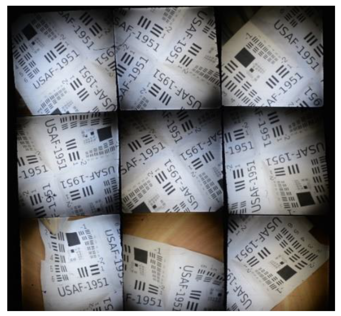
• The nine-eye bionic compound-eye system with partial overlap of fields was proposed to capture images of the target scene with fewer shots, and the image quality was improved.
• CES-MVSNet for 3D reconstruction using the bionic compound-eye system was proposed to improve the reconstruction results.
• The efficiency and reliability of using the bionic compound-eye system for 3D reconstruction were proved.

The rest of the paper is organized as follows. As mentioned above, the characteristics of the nine-eye bionic compounded-eye system and the entire experimental system are described in Section 2. The proposed method is described in detail in Section 3. Experimental results and discussion are demonstrated in Section 4. Finally, Section 5 presents the conclusions.

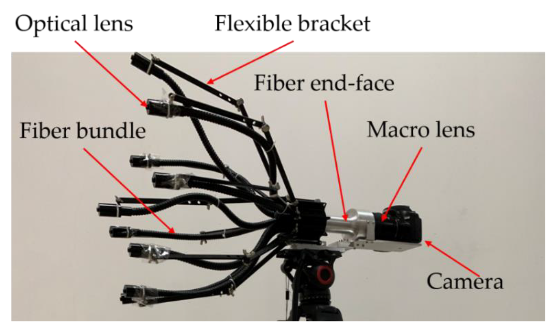
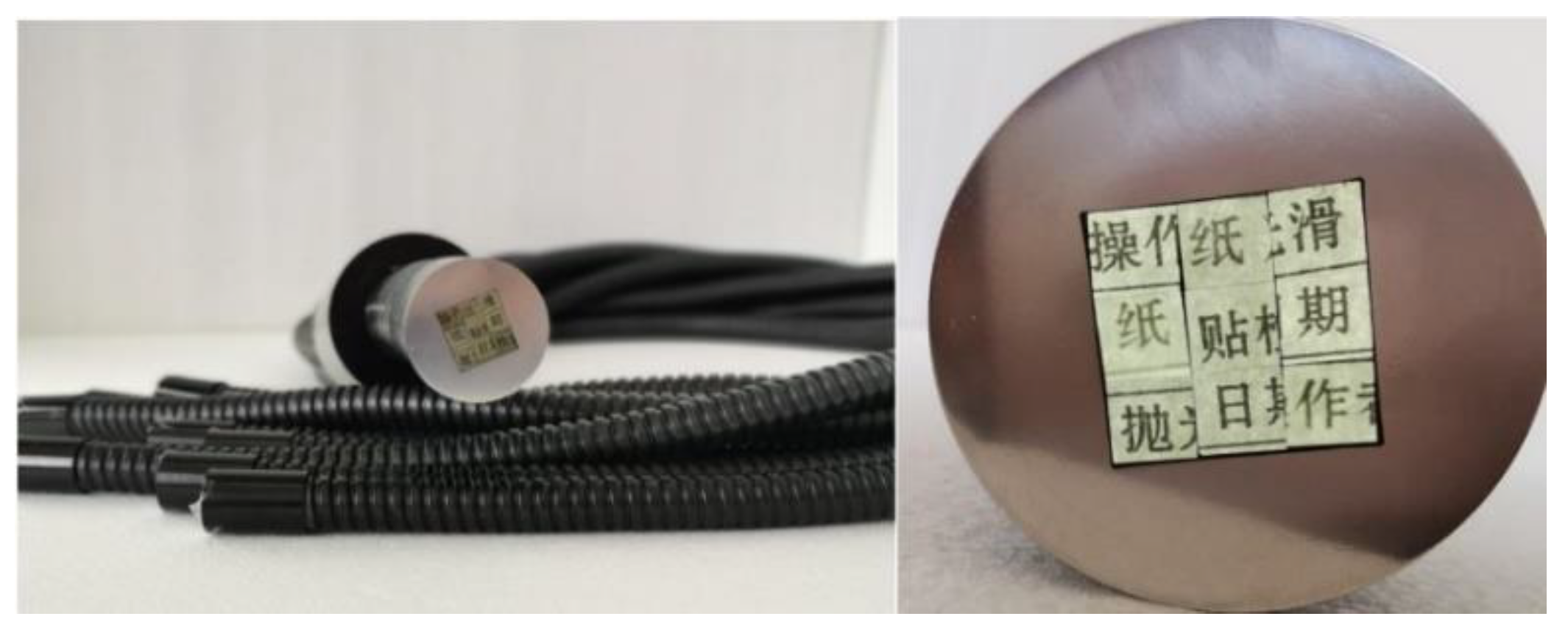
2. Nine-Eye Bionic Compound-Eye System

The structure of the nine-eye bionic compound-eye system with partial overlap of fields used in this study is shown in Figure 1. The structure of this system is similar to the compound eye structure of insects and adopts a flexible multibranch image transmission cluster mode. The front end of the flexible optical fiber has an optical lens with a field of view of 40°, distortion of less than 0.5%, focal length of 9 mm, back focal length of 4.92 mm, entrance pupil diameter of 4 mm, light transmission band of 435–656 μm, and diaphragm in the center that can be adjusted to control exposure. The end face of the optical fiber bundle is optically coupled with a camera that captures images through the sleeve. The intersecting surface of each optical fiber is square, and nine bundle clusters are connected by epoxy resin adhesive to output the image, as depicted in Figure 2. The flexible fiber bundle is fixed by two adjustable brackets that can be bent to a certain angle to control the orientation of the front lens. Owing to this octopus-like design, the baseline length between the lenses can be increased. The camera module with a macro lens is connected behind the end face of the optical fiber bundle to capture the image formed by the sub-eye lens and transmitted through the optical fiber. We used a Nikon D3200 digital SLR camera with a Nikkor 60 mm f/2.8D macro lens as the camera module, which could capture photos of 6016 × 4000 pixels. The whole system was installed on a tripod for manipulating the position and posture of the system by moving the tripod and adjusting the pan/tilt.

Owing to the design of the flexible fiber bundles for image transmission, the field-of-view overlap rate between the sub-eyes of the system can be adjusted according to the distance and scale of the object or target scene, which can make the use of the system more flexible and convenient. Whilst the images of the object or target scene are captured, a certain baseline length is maintained between the sub-eye lenses; thus, functions such as the ranging and 3D reconstruction of objects and scenes can be achieved.

An image captured by the bionic compound-eye system is shown in Figure 3. Because the gaps between the fiber bundles and the intersecting surface are not standard squares, it is necessary to perform correction processing after capturing the image of each sub-eye. In addition, the image also contains some noise and hexagonal fringes owing to the shape of the fiber material, which must be denoised and edge enhanced. At the same time, the four corners and edge areas of the image still exhibit a relatively obvious brightness drop, which requires image vignetting correction.

The luminance uniformity at different locations in the image caused by vignetting can be described by a sixth-order polynomial [16] as in Equation (1).

$$g_{a,b,c}\left(r\right)=1+ar+b{r}^2+c{r}^3+d{r}^4+e{r}^5+f{r}^6$$

(1)

The r in Equation (1) is defined by Equation (2).

$$r=\frac{\sqrt{{\left(x-x_{cm}\right)}^2+{\left(y-y_{cm}\right)}^2}}{\underset{i=0,1,2,3}{\max }\sqrt{{\left(c_{xi}-x_{cm}\right)}^2+{\left(c_{yi}-y_{cm}\right)}^2}}$$

(2)

where (x_cm, y_cm) is the center of mass of the image applied with a low-pass Gaussian filter, and (c_xi, c_yi) are the coordinates of the four corners of the image, respectively. The reason for calculating the center of mass of the image is that the optical center may not coincide with the center of the image [17]. The numerator of Equation (2) represents the Euclidean distance between the pixel and the center of mass, and the denominator is the maximum distance from the four corners of the image to the optical center to ensure that r is in the range of [0,1].

Since the intensity entropy may lead the optimization into a local optimum [18], the image log-intensity entropy is used here as the minimum criterion. First, the luminance of the image pixels L is mapped to N histogram bin i by Equation (3).

$$i\left(L\right)=\left(N-1\right)\log \left(1+L\right)/\log 256$$

(3)

The histogram bins n_k are computed by Equation (4).

$$n_k={\displaystyle \sum _{x,y:\lfloor i\left(L\left(x,y\right)\right)\rfloor =k}\left(1+k-i\left(L\left(x,y\right)\right)\right)}+{\displaystyle \sum _{x,y:\lceil i\left(L\left(x,y\right)\right)\rceil =k}\left(k-i\left(L\left(x,y\right)\right)\right)}$$

(4)

The discrete entropy is finally computed from the histogram by Equation (5).

$$H={\displaystyle \sum _k{\widehat{p}}_{k}log{\widehat{p}}_k}$$

(5)

where ${\widehat{p}}_k={\widehat{n}}_k/{\displaystyle {\sum }_j{\widehat{n}}_j}$.

We determined the best correction parameters using log-intensity entropy as the optimization criterion. The corrected image luminance is computed by Equation (6).

$$L_{corr}\left(x,y\right)=L_{orig}\left(x,y\right)g_{a,b,c}\left(r\right)$$

(6)

After the final processing, the size of the obtained image was 900 × 900 pixels, and the processing effect is shown in Figure 4. The red point is the center of mass as the optical center of the image, and the blue point is the center of the image. The correction parameters are a = 0.012, b = 0.03, c = 0.17, d = 0.448, e = 0.942, and f = 5.661, respectively. The log-intensity entropy of the images before and after correction decreased from 6.65112 to 5.90766. It can also be seen that the luminance uniformity was significantly improved after correction.

We used NVIDIA Jetson AGX Xavier to process the images captured by the compound-eye system and run the 3D reconstruction algorithm, as shown in Figure 5. Jetson AGX Xavier is an intelligent development kit from NVIDIA. Compared with the previous generation Jetson TX2, the performance was improved by more than 20 times, and the energy efficiency was improved by a factor of 10. Furthermore, it can support algorithms, such as visual SLAM, obstacle detection, and path planning. A diagram of the entire system is shown in Figure 6.

3. Method of 3D Reconstruction Using a Bionic Compound-Eye System

3.1. Traditional Method

The traditional 3D reconstruction method is based on the principle of multi-view geometry and estimates the depth of the point in view by triangulation. The projective geometry between the two views is called epipolar geometry [19], which describes the relationship between the projected points and projected rays of points in space in different views, as depicted in Figure 7. According to the epipolar geometric constraints of different views, the spatial position of the pixel point can be obtained, and two parts of the information must be known for the calculation. The first is to determine the pixel positions of the same point in space for different views, that is, to perform feature matching between images. There are different types of image features: First, SIFT, which has scale-invariant image features, is a good choice for the algorithm to identify the corresponding features in multiple different images. Second, the state of the camera when capturing different views must be known, that is, the intrinsic and motion matrices of the camera must be known. To obtain this information, camera calibration must be performed.

Many mature calibration algorithms are available for the calibration of camera parameters, such as the calibration method proposed by Zhang [20]. In the 3D reconstruction method with a fixed camera configuration, the camera parameters only need to be calibrated once, and the same parameters can be used for subsequent calculations. The position of the sub-eye lens can be adjusted freely for the compound-eye system. However, during the image-capturing process, the entire system is in consistent motion. The camera parameters must be recalibrated after each shot. However, if a calibration object, such as the checkerboard, is used, the entire shooting process becomes very cumbersome, and at the same time, more images need to be processed, as mentioned above. Therefore, in this work, we restore the camera parameters by solving the Perspective-n-Point (PnP) problem [21], which does not need to shoot the calibration object after each movement of the system but directly uses the image of the subject or scene captured by the system.

3.2. CES-MVSNet: Method of 3D Reconstruction Using a Nine-Eye Bionic Compound-Eye System

In this study, we adopted an incremental method owing to its good reconstruction performance. The main steps of the algorithm are as follows: first, extract and match the feature points between two images, estimate two-view reconstruction, use it as the initialization of the reconstruction, continuously add new images to the current model, and perform triangulation and bundle adjustment to refine the final 3D model. When choosing the initial pair at the initialization stage, the images should have a large number of matches and a large baseline [22]. The advantage of using a bionic compound-eye system for 3D scene reconstruction is that, by adjusting and controlling the angles between the sub-eyes of the system, even if the system is constantly moved, the success rate of establishing good two-view initialization can be guaranteed, which is convenient for further steps.

The time complexity of the incremental method is typically O(n⁴), and the main time consumption lies in the increasing number of input images, which leads to an increase in the time required for image matching and nonlinear optimization of the bundle adjustment [23].

Deep-learning networks have unique advantages for the prediction and reconstruction of 3D spatial shapes by learning and mining deeper structural features. Three-dimensional reconstruction through deep learning is essentially carried out through prediction of the depth value of the pixel point. The general processing method regards the estimation of the depth value as a typical classification problem, uses different depth values within a certain depth range as different depth hypotheses, estimates the probability of each depth estimation, and finally calculates the expectation depth value along the depth direction to obtain the depth of the pixel.

Based on the basic structure of the MVSNet, in this study, we designed a deep neural network of the bionic compound-eye system named CES-MVSNet. The network structure is illustrated in Figure 8.

3.2.1. Feature Extraction

First, extract the image features {I_i${\}}_{i=1}^N$ of the input image {F_i${\}}_{i=1}^N$, where N represents the total number of input images. Since the resolution of the images captured by the compound-eye system is relatively low, in order to extract higher-order image features while ensuring computational efficiency, compared with the eight-layer convolutional network in MVSNet, CES-MVSNet uses a nine-layer convolutional as shown in

Table 1. Detailed architecture of the feature extraction network.

Input	Layer	Output	Output Size
Ii	Conv2D + BN + ReLU, K = 3 × 3, S = 1, F = 8	2D_0	H × W × 8
2D_0	Conv2D + BN + ReLU, K = 3 × 3, S = 1, F = 8	2D_1	H × W × 8
2D_1	Conv2D + BN + ReLU, K = 5 × 5, S = 2, F = 16	2D_2	½H × ½W × 16
2D_2	Conv2D + BN+ReLU, K = 3 × 3, S = 1, F = 16	2D_3	½H × ½W × 16
2D_3	Conv2D + BN + ReLU, K = 3 × 3, S = 1, F = 16	2D_4	½H × ½W × 16
2D_4	Conv2D + BN + ReLU, K = 5 × 5, S = 2, F = 32	2D_5	¼H × ¼W × 32
2D_5	Conv2D + BN + ReLU, K = 3 × 3, S = 1, F = 32	2D_6	¼H × ¼W × 32
2D_6	Conv2D + BN + ReLU, K = 3 × 3, S = 1, F = 32	2D_7	¼H × ¼W × 32
2D_7	Conv2D + BN + ReLU, K = 3 × 3, S = 1, F = 32	Fi	¼H × ¼W × 32

, where K denotes the kernel size, S the kernel stride, F the number of output channels, and H and W the width and height of the image, respectively. A batch-normalization (BN) layer and a Leaky-ReLU layer are added after each convolutional layer.

3.2.2. Build Cost Volume

After obtaining the extracted image features, it is necessary to construct an image-matching cost volume for depth estimation from the reference view. Assuming that the depth range covered by the scene in the reference view is [d_min, d_max], this depth range was evenly divided into M different depth hypotheses to construct the cost volume. Each depth hypothesis is d_m = d_min + m(d_max − d_min)/M, where m∈{0,1,2,…,M − 1}, representing the different fronto-parallel planes of the reference camera.

The relationship between pixel x in the reference view and corresponding pixel x_i in the ith source view can be expressed using differentiable homography [9], as in Equation (7).

$${\mathbf{H}}_i\left(d\right)={\mathbf{K}}_i{\mathbf{R}}_i\left(\mathbf{I}-\frac{\left({\mathbf{R}}_i{\mathbf{t}}_i-{\mathbf{R}}_0^{-1}{\mathbf{t}}_0\right){\mathbf{n}}_0^T{\mathbf{R}}_0}{d}\right){\mathbf{R}}_0^{-1}{\mathbf{K}}_0^{-1}$$

(7)

where I denotes the identity matrix, and K, the intrinsic matrix of the camera. This correspondence can be expressed as λ_i·x_i = H_i(d)·x, where λ_i represents the depth of x_i in the ith source view.

At a plane of depth d, the matching cost of all pixels is defined as the variance of all features in N views, as in Equation (8).

$$c_d=\frac{1}{N}{\displaystyle \sum _{i=0}^N{\left(F_{i,d}-F_d\right)}^2}$$

(8)

where F_i,d denotes the feature maps that are transformed from the source view into the reference view by bilinear interpolation, and F_d is the expectation of the feature volume of each pixel in all views.

When using the compound-eye system, we can adjust the number of shots for different scenes to improve the reconstruction effect. Using variance can leverage any number of image inputs while balancing image-feature differences among multiple views to satisfy photometric consistency constraints. The matching cost of each depth hypothesis is calculated and concatenated to obtain the cost volume, which has a size of H/4 × W/4 × M × C, where C is the number of channels of the feature map.

3.2.3. Depth Map Estimation

The resulting cost volume is fed into a 3D U-Net [24] that outputs the depth probability volume. Unlike the 3D U-Net of MVSNet, which uses convolutional layers with a convolution kernel size of 3 × 3 × 3, on shallow layers, anisotropic convolutional layers with convolution kernel sizes of 3 × 3 × 1 and 5 × 5 × 1 were adopted to fuse the information on each depth hypothesis plane, which are equivalent to 2D convolution with convolution kernels of 3 × 3 and 5 × 5 on each depth hypothesis plane. The purpose of using two kernel sizes is to extract global and local information at the same time. We also use anisotropic convolutional layers with convolution kernel sizes of 1 × 1 × 7 to enlarge the receptive field along the depth direction with less memory usage and computation. In the deeper layers, as well as the output layer, an isotropic convolutional layer with a kernel size of 3 × 3 × 3 was used to fuse more contextual information [25]. The detailed architecture of the 3D U-Net of CES-MVSNet is shown in

Table 2. Detailed architecture of the 3D U-Net.

Input	Layer	Output	Output Size
C	Conv3D + BN + ReLU, K = 3 × 3 × 1, S = 1, F = 8	3D_0	¼H × ¼W × D × 8
3D_0	Conv3D + BN + ReLU, K = 1 × 1 × 7, S = 2, F = 16	3D_1	⅛H × ⅛W × ½D × 16
3D_1	Conv3D + BN + ReLU, K = 5 × 5 × 1, S = 1, F = 16	3D_2	⅛H × ⅛W × ½D × 16
3D_2	Conv3D + BN + ReLU, K = 1 × 1 × 7, S = 2, F = 32	3D_3	1/16H × 1/16W × ¼D × 32
3D_3	Conv3D + BN + ReLU, K = 3 × 3 × 1, S = 1, F = 32	3D_4	1/16H × 1/16W × ¼D × 32
3D_4	Conv3D + BN + ReLU, K = 1 × 1 × 7, S = 2, F = 64	3D_5	1/32H × 1/32W × ⅛D × 64
3D_5	Conv3D + BN + ReLU, K = 3 × 3 × 3, S = 1, F = 64	3D_6	1/32H × 1/32W × ⅛D × 64
3D_6	Deconv3D + BN + ReLU, K = 3 × 3 × 3, S = 2, F = 32	3D_7	1/16H × 1/16W × ¼D × 32
3D_7 + 3D_4	Addition	3D_8	1/16H × 1/16W × ¼D × 32
3D_8	Deconv3D + BN + ReLU, K = 1 × 1 × 7, S = 2, F = 16	3D_9	⅛H × ⅛W × ½D × 16
3D_9 + 3D_2	Addition	3D_10	⅛H × ⅛W × ½D × 16
3D_10	Deconv3D + BN + ReLU, K = 3 × 3 × 1, S = 2, F = 16	3D_11	¼H × ¼W × D × 8
3D_11 + 3D_0	Addition	3D_12	¼H × ¼W × D × 8
3D_12	Conv3D, K = 3 × 3 × 3, S = 1, F = 1	P	¼H × ¼W × D

, where D denotes the depth sample number.

To be able to generate continuous depth estimation, a soft-max operation on the probability volume along the depth direction to obtain the estimated depth map must be performed; then, the depth estimation of pixel x can be expressed as in Equation (9).

$$D\left(x\right)={\displaystyle \sum _{m=0}^{M-1}{d}_m{P}_x\left(d_m\right)}$$

(9)

3.2.4. Loss Function

To select the loss function, we used the l1 norm as a measure of the mean absolute error between the ground truth and estimated depth map. For each training sample, the training loss can be expressed as Equation (10).

$$Loss={\displaystyle \sum _{x\in {\Omega }_{valid}}{\Vert D_{gt}\left(x\right)-D\left(x\right)\Vert }_1}$$

(10)

where Ω_valid represents the set of pixels with the ground-truth depth information in view.

After the network training was completed, we fed the images that needed to be reconstructed and the corresponding camera parameters to the network. Each image was used as a reference to obtain an estimated depth map. Finally, the depth map was re-projected to obtain the final 3D reconstructed point cloud model [26].

4. Experiments

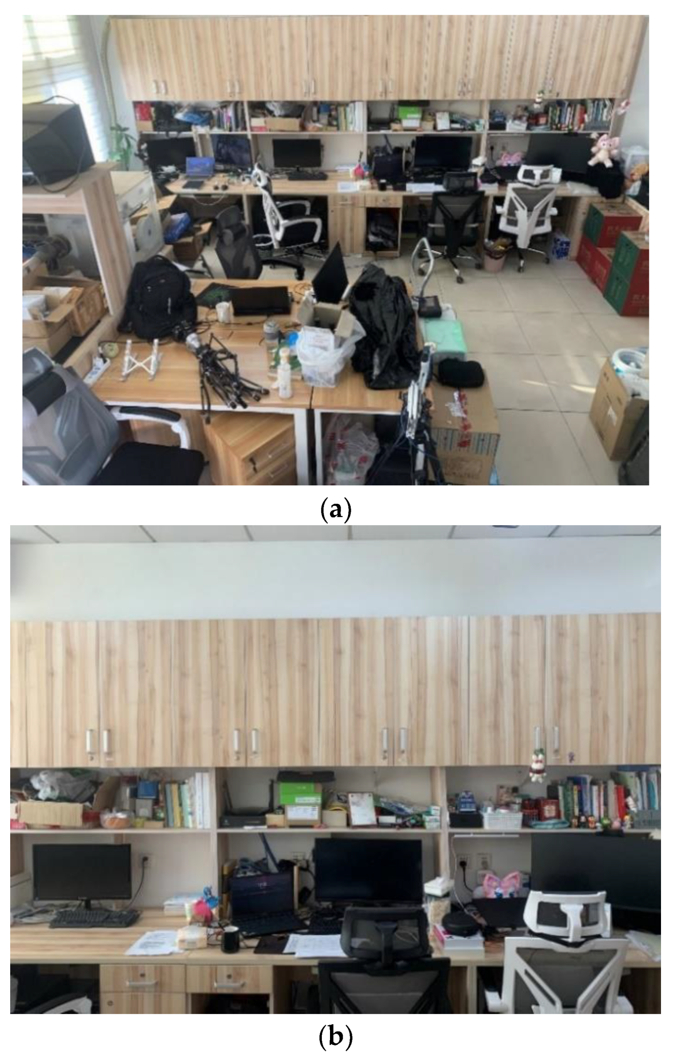
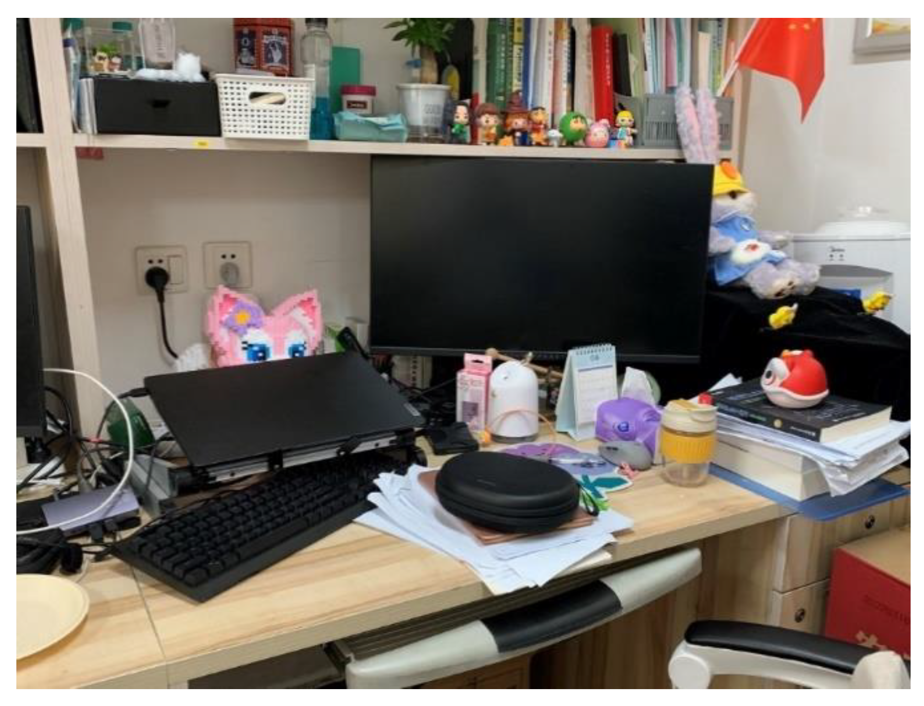
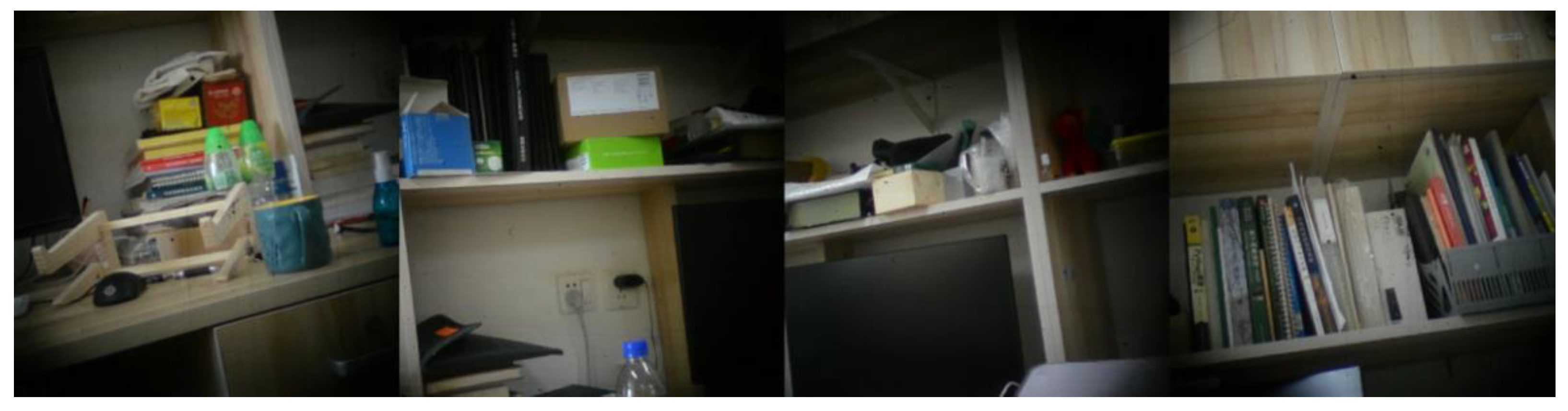
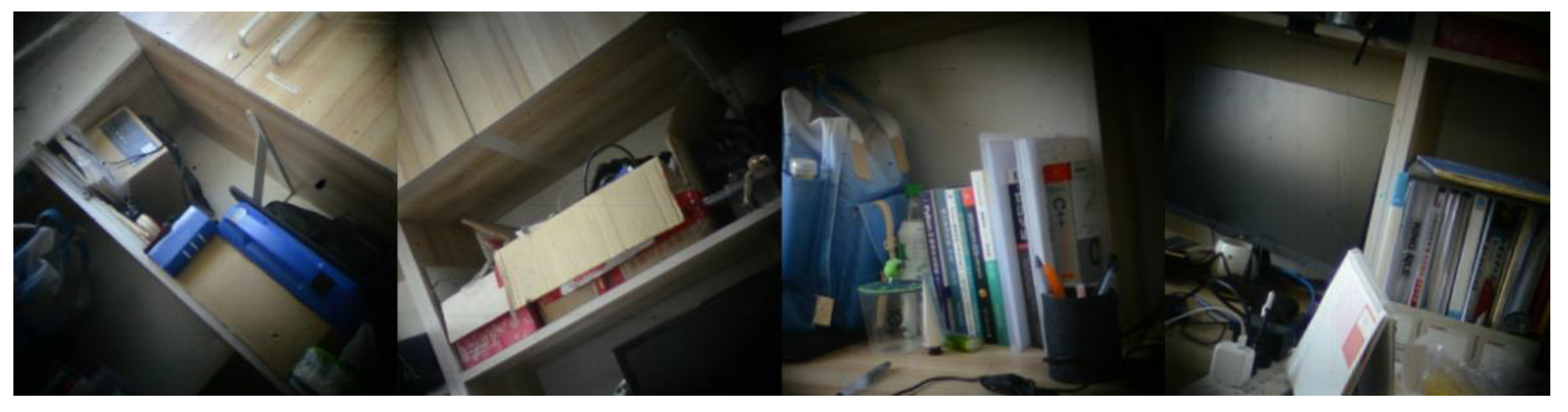
4.1. System and Scene

We installed the whole system on a tripod and manipulated the position and posture of the system by moving the tripod and adjusting the pan/tilt. Imaging of the experiment was conducted in a laboratory room with an area of approximately 6 m × 6 m. The indoor layout was relatively simple, and the furnishings were rich and varied, as shown in Figure 9.

4.2. Training

Similar to the training MVSNet [9], the training dataset was divided into three parts: the training set, validation set, and test set. The BlendedMVS datasets were used to train the network to test and enhance the generalization ability of the neural network for different scenes.

The BlendedMVS dataset [27] is a large-scale MVS dataset for multi-view 3D reconstructions, as shown in Figure 10. The dataset contained 17,000 MVS training samples covering 113 scenes, including large buildings, sculptures, and small objects. The BlendedMVS dataset was a synthetic dataset. A 3D model was generated from the image using Altizure, an online 3D reconstruction platform, and output the rendered image and depth map from different viewpoints according to the model. The input image was applied with a low-pass filter to extract ambient light information, and the rendered image was applied with a high-pass filter to extract image-edge information. Then, the two results were linearly fused to obtain a fused image.

We used Pytorch 1.6.0 and an NVIDIA RTX3080ti GPU to train CES-MVSNet. Then, we used an NVIDIA Jetson AGX Xavier to process the captured images and run the 3D reconstruction algorithm to simulate the practical application scenarios and verify the proposed method in this paper.

The network training used an Adam optimizer; the batch size was set to 2 with an initial learning rate of 0.001. The total epochs were set to 15, and the learning rate scheduler was set to cosine.

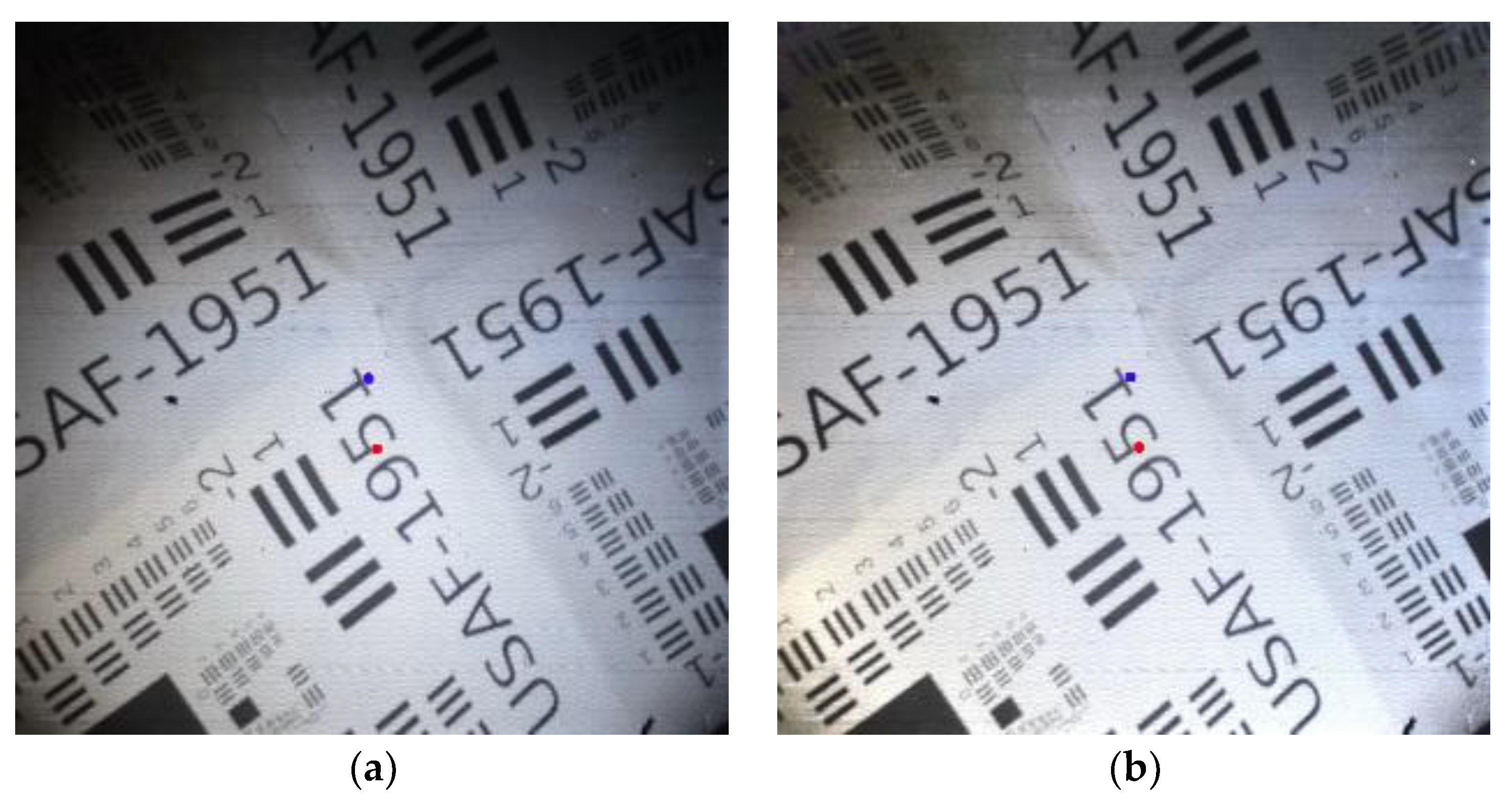
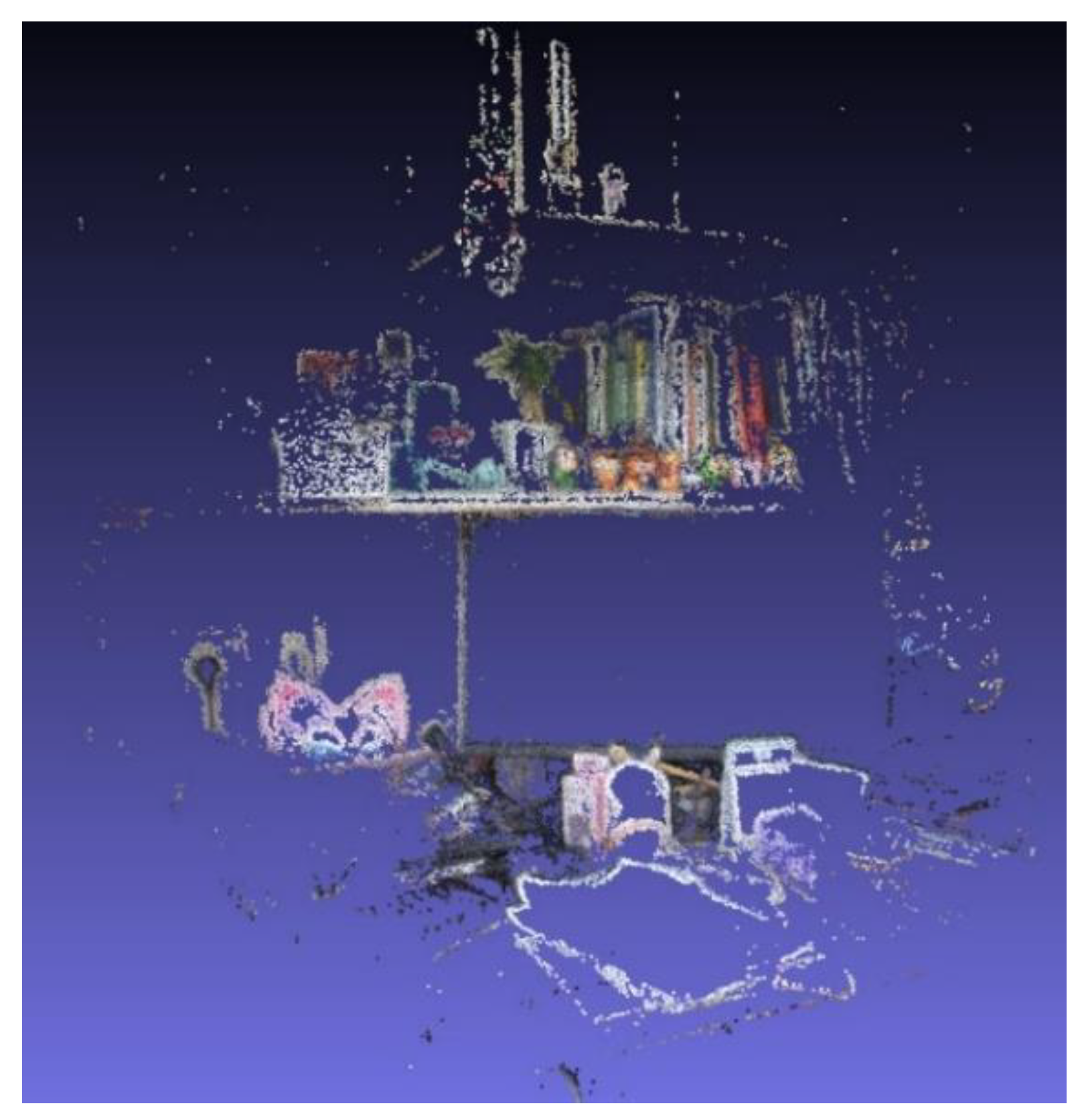
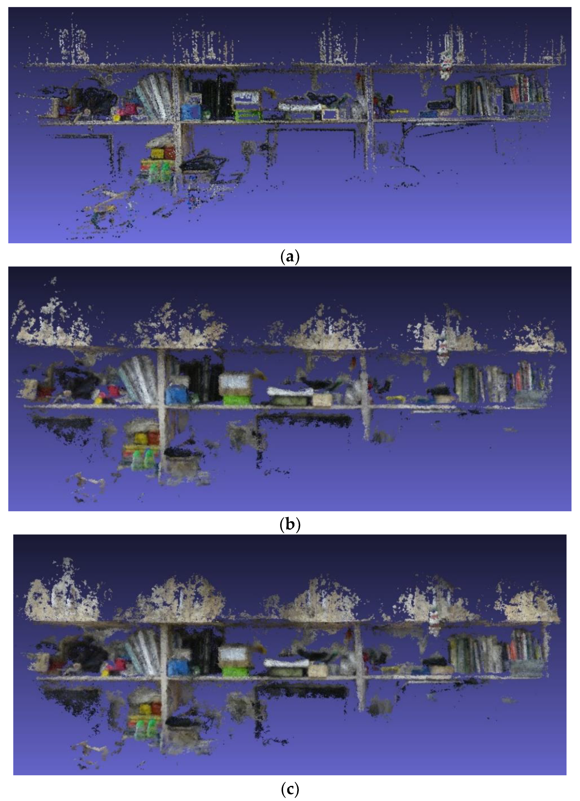
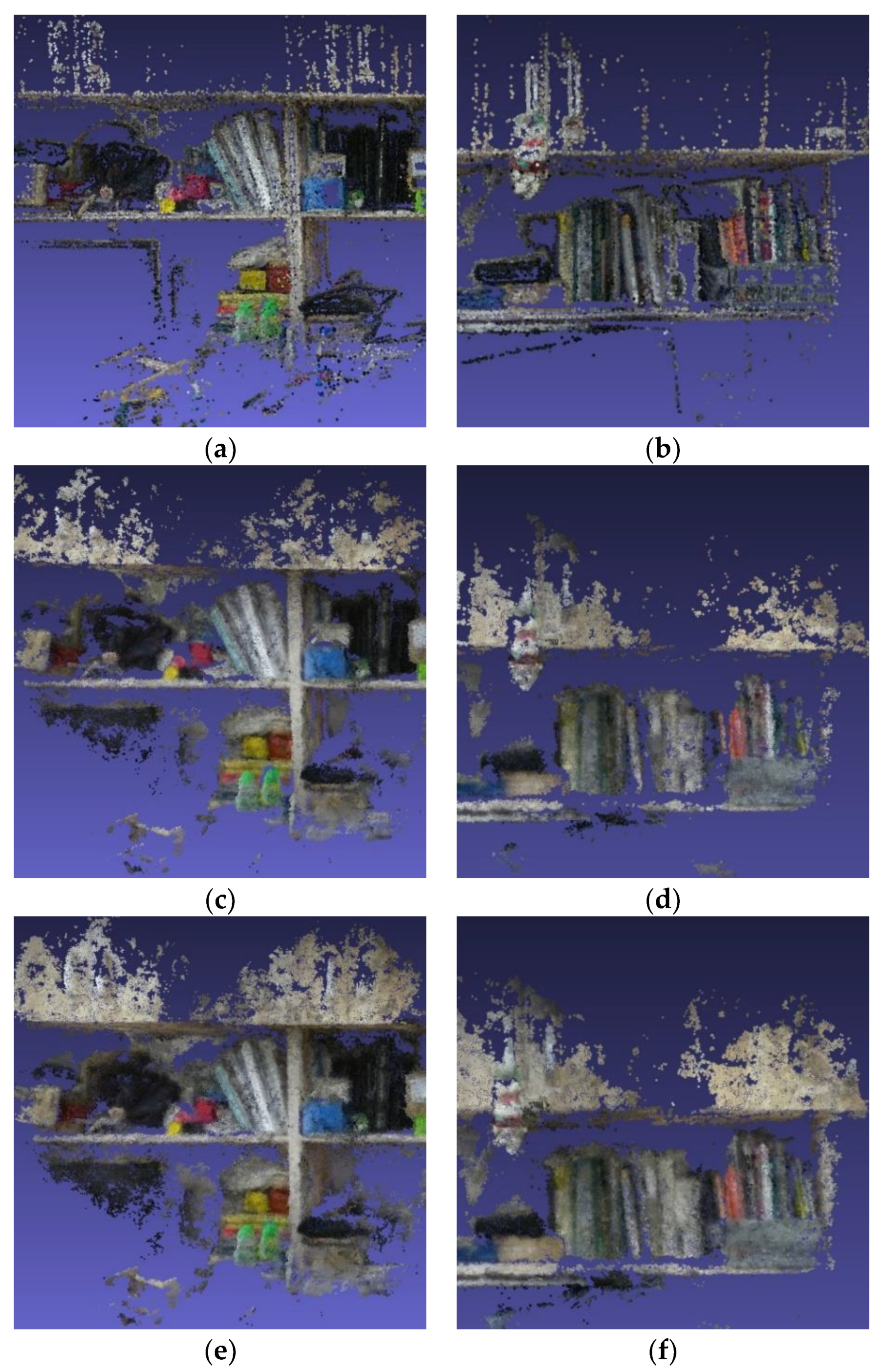
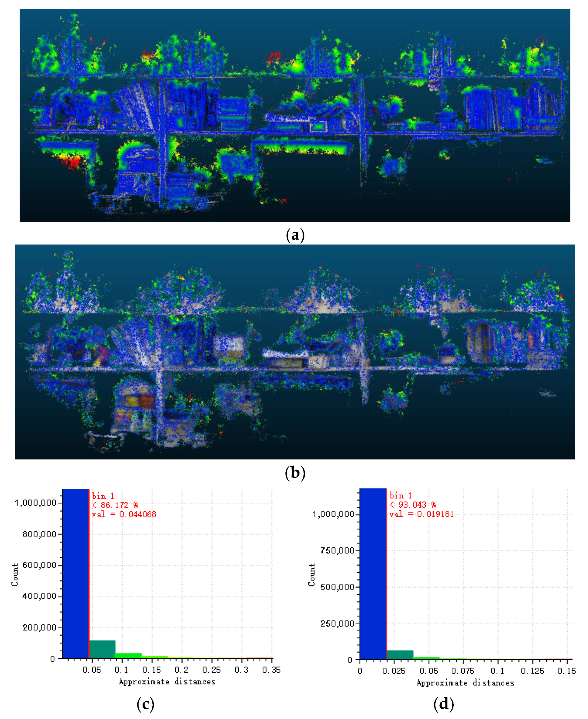
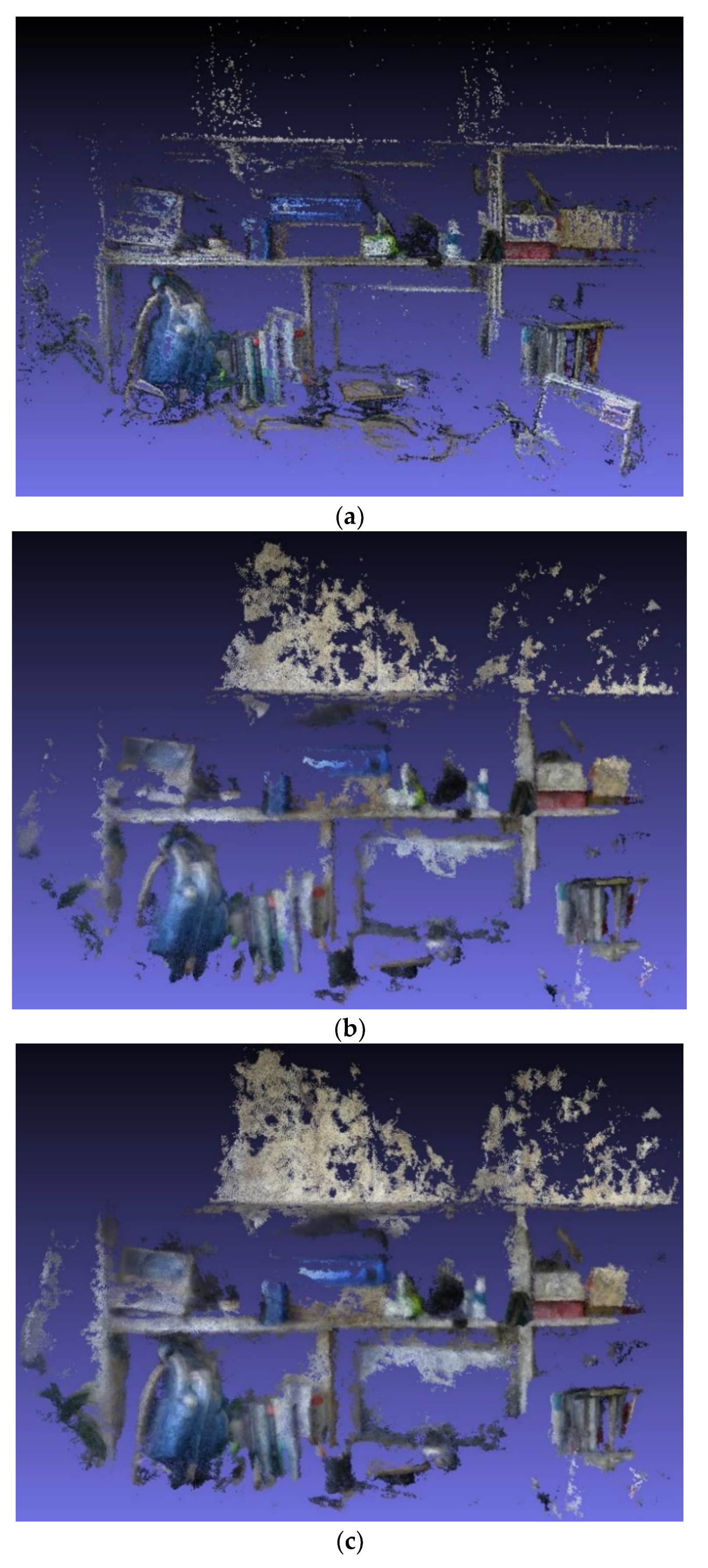
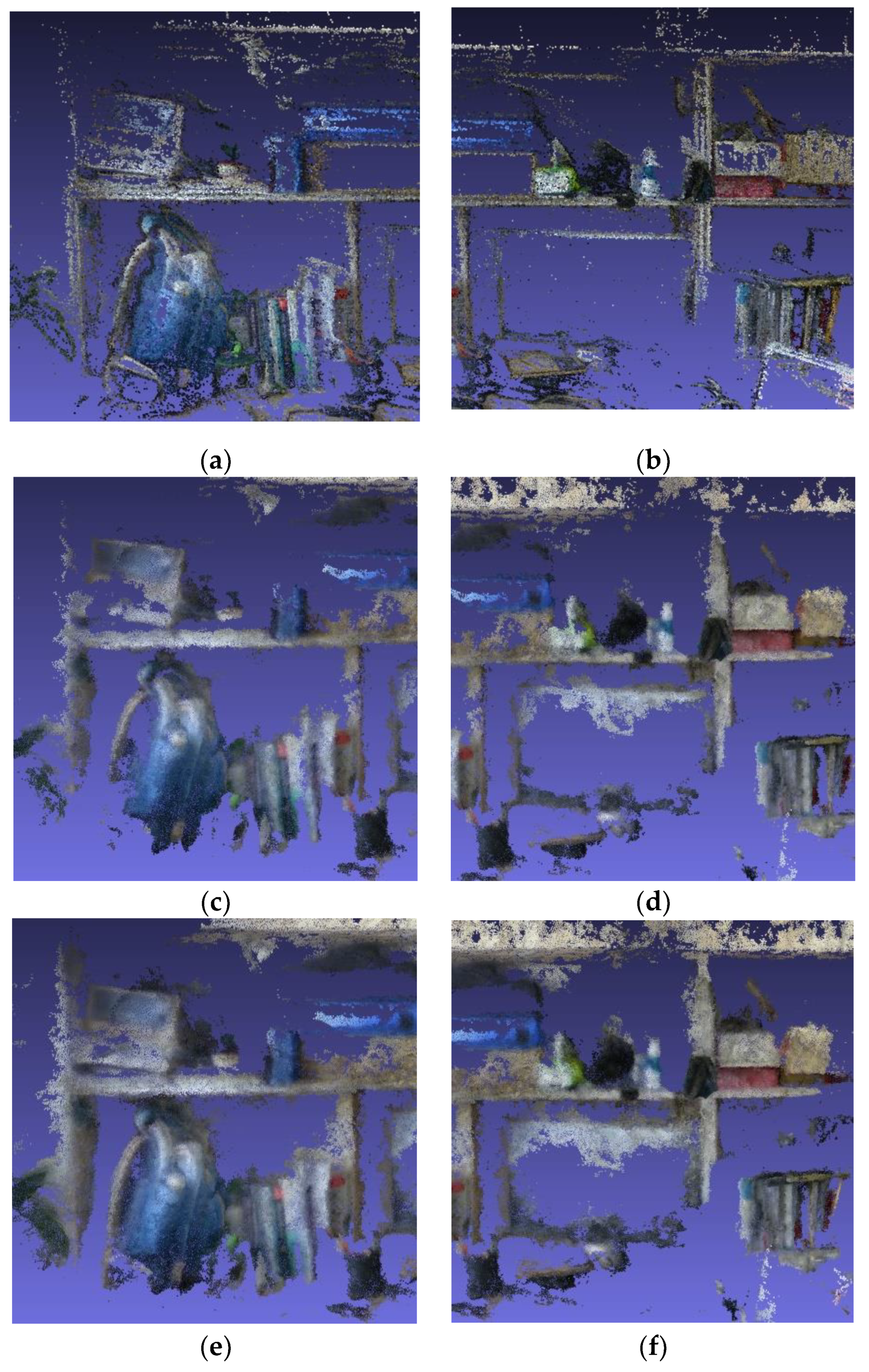
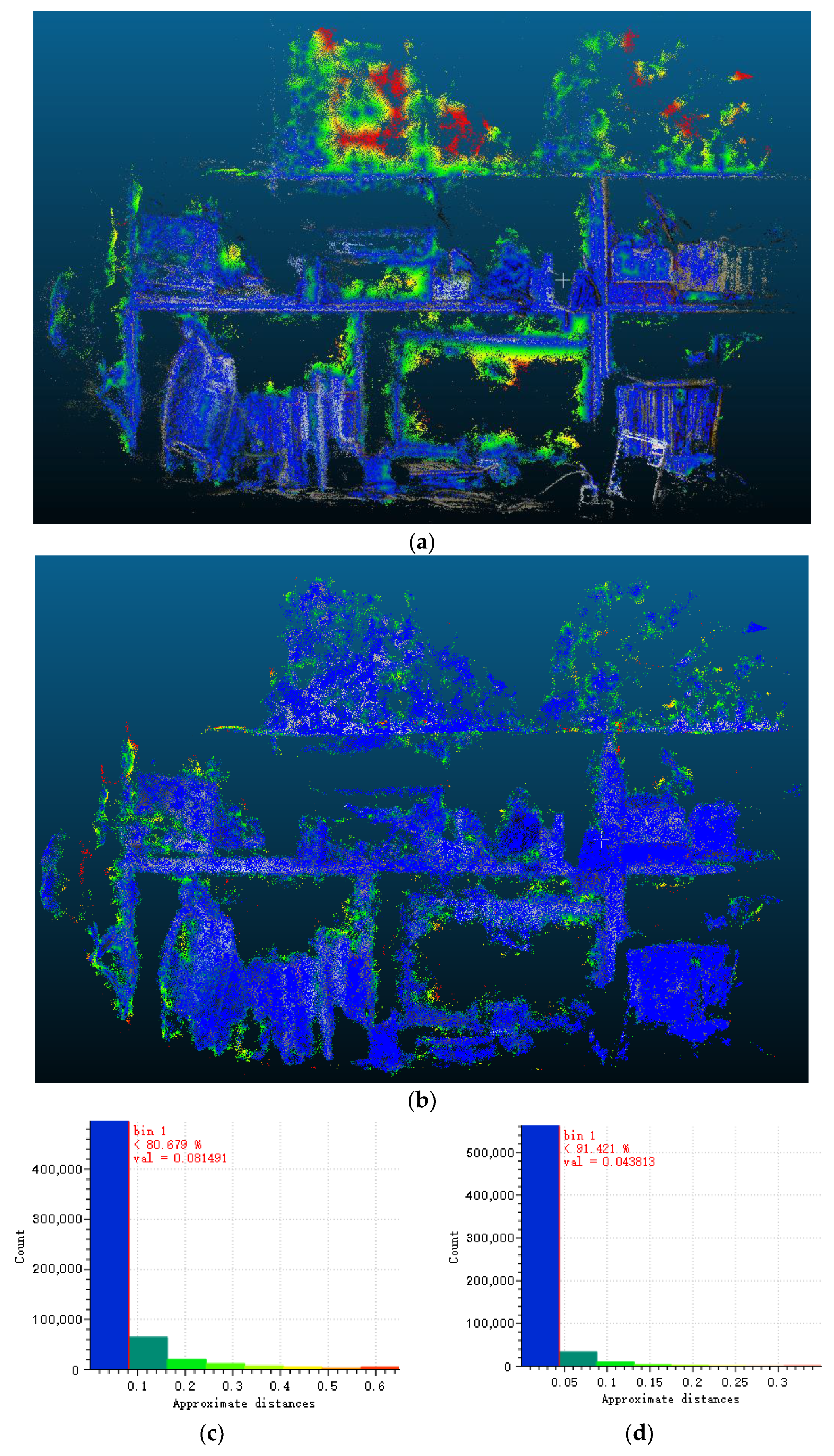
4.3. Experiment with Compound-Eye System and Discussion

In order to prove the efficiency and reliability of the 3D scene reconstruction using the bionic compound-eye system, we captured a scene in the laboratory room, which is shown in Figure 11, using the compound-eye system and a monocular camera, respectively. When shooting with the bionic compound-eye system, the relative positions of the sub-eye lenses of the system remained fixed, and the sub-eye images maintained a partial overlap of fields. The system was slightly moved to shoot five times from different angles and distances, and a total of 45 images were obtained for 3D reconstruction. When shooting with a monocular camera, the relative position of the camera between each shot was not limited, and multiple shots were taken from different angles and distances. The program automatically selected 45 available images from the initial input images. The 3D reconstruction results of the bionic compound-eye system and the monocular camera are shown in Figure 12 and Figure 13, respectively.

For the images captured by the bionic compound-eye system, the relative positions of the sub-eye lenses of the system were fixed, and all images obtained by shooting five times could be successfully matched and reconstructed. For the images captured by the monocular camera, some images failed to match with other images, so the reconstruction could not be performed successfully. From the initial input of 54 images, the same number of 45 images could be selected for reconstruction by the program. By comparing the results, the reconstruction of images captured by the bionic compound eye included about 110,000 points, which is better than that of the monocular camera with about 73,000 points.

A similar experiment was performed on another narrower scene in the laboratory. The experimental scene is shown in Figure 14, and the reconstruction results of the bionic compound-eye system and the monocular camera are shown in Figure 15 and Figure 16, respectively. The bionic compound-eye system was used for 3 shots, and a total of 27 images were obtained. The number of initial inputs of monocular camera images was 32, and 27 images were finally selected for reconstruction. The number of points of the two reconstruction results was about 104,000 and 62,000, respectively, and the number of reconstruction points of the bionic compound-eye system was slightly more than that of the monocular camera. The experimental results also showed that 3D reconstruction for a smaller scene can be achieved using a smaller number of images.

After several experiments, it was verified that all the images captured by the bionic compound-eye system could be used for 3D reconstruction, while a small part of the images captured by a monocular camera could not. The bionic compound-eye system has nine sub-eyes, so the shooting efficiency of using the bionic compound-eye system is nine times that of using a monocular camera. In the case of using the same number of images for reconstruction, the reconstruction effect of the bionic compound-eye system is close to or even slightly better than that of a monocular camera in terms of visual effects, and the number of reconstruction points of the former is about 50% more than that of the latter. Therefore, using the bionic compound-eye system for 3D reconstruction can effectively improve the shooting efficiency and, at the same time, achieve the 3D reconstruction effect consistent with using a monocular camera.

In order to compare the difference between the effects of different reconstruction methods, we used the compound-eye system to capture two wider scenes in the laboratory room, and 144 and 81 images were selected for each scene. Some of the processed captured images of scene 1 are shown in Figure 17, and the overall and detailed 3D models reconstructed by different methods are shown in Figure 18 and Figure 19, respectively.

We also use cloud compare software to analyze the results reconstructed by different methods, as shown in Figure 20. We compute the approximate distances of each point of the compared cloud relative to the reference cloud. The compared cloud is colored with the approximate distances. The histogram of the compared cloud shows that the points with green, yellow, and red colors, which indicate larger approximate distances, can be seen as the parts that are not well recovered in the reference cloud. As shown in Figure 20c,d, the ratios of the points with their colors were about 14% and 7%, respectively, which shows that the proposed method outperforms the previous methods in terms of completeness.

Some of the processed captured images of scene 2 are shown in Figure 21, and the overall and detailed 3D models reconstructed by different methods are shown in Figure 22 and Figure 23, respectively. The computed cloud-to-cloud distance results are shown in Figure 24.

The results of the two different networks show that the reconstruction details and completeness of the model obtained by CES-MVSNet are significantly improved compared to the model obtained by MVSNet. Additionally, a comparison of the results of the two different methods shows that the completeness of the model obtained using the neural network was generally better than those obtained using the traditional method. The resolution of the traditional method was higher. However, the model contains more obvious outliers. The distribution of point clouds is relatively loose, especially in areas with fewer texture features, such as the surface of the top lockers, which have very vague details. The computer monitor below was almost invisible, but its black edges were still visible, and a few points in the part of the screen panel were not on the same spatial plane. Although the results of the deep learning network are slightly blurry, it can retain more detail in areas with fewer texture features compared to the former result, and the model had higher integrity and smoother visual effects. The two methods can achieve a relatively good recovery of the basic shape and relative positional relationship of the object, and generally, there were no obvious errors. Because the probability volume was used in the deep learning method, it can be used as a confidence measure for depth estimation. The confidence threshold can be set during the reconstruction process, and points with low confidence can be filtered to obtain reconstructed points with high confidence. Neither of the methods could reconstruct more subtle features well, such as some text on the spine of the book or on the box, but this is determined more by the resolution of the optical lens of the system and the quality of the image acquisition.

In terms of the running time of the algorithm, using the traditional method to obtain a relatively good 3D reconstruction required about 100 more images and 1~2 h each time, which is determined by the accuracy of the feature extraction and optimization operations, whereas using a pre-trained deep neural network requires a few minutes, which is more efficient than the traditional method. The training time of the deep learning network on the RTX 3080Ti graphics card could also be controlled within 20 h.

5. Conclusions

This study investigated 3D reconstruction using a nine-eye bionic compound-eye system with a partial overlap of fields and proposed CES-MVSNet for 3D reconstruction using our system. We fed the captured image and camera parameters to the trained deep neural network, which can generate a 3D reconstruction result quickly. The difference between the effects of the traditional multi-view geometric method and neural networks for 3D reconstruction was analyzed, which proved that using the bionic compound-eye system for 3D reconstruction can greatly improve the efficiency while ensuring the success rate of reconstruction tasks and the integrity and accuracy of the reconstruction results.

In the future, the main research direction of 3D reconstruction using the bionic compound-eye system is to further improve the completeness and accuracy of the resulting model, and further improvements to the imaging quality of the optical system and integration of the whole system will be pursued. The high-quality 3D reconstruction of the scene obtained by the bionic compound-eye system has broad application prospects in automated vehicle recognition, map drawing, robot navigation, and obstacle avoidance.

References

1. Arie-Nachimson, M.; Kovalsky, S.Z.; Kemelmacher-Shlizerman, I.; Singer, A.; Basri, R. Global Motion Estimation from Point Matches. In Proceedings of the 2012 Second International Conference on 3D Imaging, Modeling, Processing, Visualization & Transmission, Zurich, Switzerland, 13–15 October 2012; pp. 81–88. [Google Scholar]
2. Shah, R.; Deshpande, A.; Narayanan, P.J. Multistage SFM: A Coarse-to-Fine Approach for 3D Reconstruction. arXiv 2015, arXiv:1512.06235. [Google Scholar]
3. Snavely, N.; Seitz, S.M.; Szeliski, R. Photo Tourism: Exploring image collections in 3D. ACM Trans. Graph. 2006, 25, 835–846. [Google Scholar] [CrossRef]
4. Schönberger, J.L.; Frahm, J.M. Structure-from-Motion Revisited. In Proceedings of the IEEE Conference on Computer Vision & Pattern Recognition, Las Vegas, NV, USA, 27–30 June 2016; pp. 4104–4113. [Google Scholar]
5. Chen, Y.; Chan, A.B.; Lin, Z.; Suzuki, K.; Wang, G. Efficient tree-structured SfM by RANSAC generalized Procrustes analysis. Comput. Vis. Image Underst. 2017, 157, 179–189. [Google Scholar] [CrossRef]
6. Cui, H.; Gao, X.; Shen, S.; Hu, Z. HSfM: Hybrid Structure-from-Motion. In Proceedings of the IEEE Conference on Computer Vision & Pattern Recognition, Honolulu, HI, USA, 21–26 July 2017; pp. 2393–2402. [Google Scholar]
7. Zhu, S.; Zhang, R.; Zhou, L.; Shen, T.; Fang, T.; Tian, P.; Quan, L. Very Large-Scale Global SfM by Distributed Motion Averaging. In Proceedings of the 2018 IEEE Conference on Computer Vision and Pattern Recognition (CVPR), Salt Lake City, UT, USA, 18–23 June 2018; pp. 4568–4577. [Google Scholar]
8. Eigen, D.; Puhrsch, C.; Fergus, R. Depth Map Prediction from a Single Image using a Multi-Scale Deep Network. In Proceedings of the 27th International Conference on Neural Information Processing System (NIPS), Montreal, QC, Canada, 8–13 December 2014; Volume 2, pp. 2366–2374. [Google Scholar]
9. Yao, Y.; Luo, Z.; Li, S.; Fang, T.; Quan, L. MVSNet: Depth Inference for Unstructured Multi-view Stereo. Lect. Notes Comput. Sci. 2018, 8, 785–801. [Google Scholar]
10. Chen, R.; Han, S.; Xu, J.; Su, H. Point-Based Multi-View Stereo Network. In Proceedings of the International Conference on Computer Vision, Seoul, Korea, 27–28 October 2019; pp. 1538–1547. [Google Scholar]
11. Yi, H.; Wei, Z.; Ding, M.; Zhang, R.; Chen, Y.; Wang, G.; Tai, Y. Pyramid multi-view stereo net with self-adaptive view aggregation. In Proceedings of the European Conference on Computer Vision, Glasgow, UK, 23–28 August 2020; pp. 766–782. [Google Scholar]
12. Yao, Y.; Luo, Z.; Li, S.; Shen, T.; Fang, T.; Quan, L. Recurrent mvsnet for high-resolution multi-view stereo depth inference. In Proceedings of the IEEE/CVF Conference on Computer Vision and Pattern Recognition, Long Beach, CA, USA, 15–20 June 2019; pp. 5525–5534. [Google Scholar]
13. Yan, J.; Wei, Z.; Yi, H.; Ding, M.; Zhang, R.; Chen, Y.; Wang, G.; Tai, Y. Dense hybrid recurrent multi-view stereo net with dynamic consistency checking. In Proceedings of the European Conference on Computer Vision, Glasgow, UK, 23–28 August 2020; pp. 674–689. [Google Scholar]
14. Gu, X.; Fan, Z.; Zhu, S.; Dai, Z.; Tan, F.; Tan, P. Cascade cost volume for high-resolution multi-view stereo and stereo matching. In Proceedings of the IEEE/CVF Conference on Computer Vision and Pattern Recognition, Seattle, WA, USA, 13–19 June 2020; pp. 2495–2504. [Google Scholar]
15. Cheng, S.; Xu, Z.; Zhu, S.; Li, Z.; Li, E.; Ramamoorthi, R.; Su, H. Deep stereo using adaptive thin volume representation with uncertainty awareness. In Proceedings of the IEEE/CVF Conference on Computer Vision and Pattern Recognition, Seattle, WA, USA, 13–19 June 2020; pp. 2524–2534. [Google Scholar]
16. Goldman, D.B.; Chen, J. Vignette and Exposure Calibration and Compensation. IEEE Trans. Pattern Anal. Mach. Intell. 2010, 32, 2276–2288. [Google Scholar] [CrossRef] [PubMed]
17. Lopez-Fuentes, L.; Oliver, G.; Massanet, S. Revisiting Image Vignetting Correction by Constrained Minimization of Log-Intensity Entropy. Adv. Comput. Intell. 2015, 9095, 450–463. [Google Scholar]
18. Rohlfing, T. Single-Image Vignetting Correction by Constrained Minimization of log-Intensity Entropy. In Lecture Notes in Computer Science; Springer: Cham, Switzerland, 2012; pp. 450–463. [Google Scholar]
19. Hartley, R.; Zisserman, A. Multiple View Geometry in Computer Vision, 2nd ed.; Cambridge University Press: Cambridge, UK, 2003; pp. 239–241. [Google Scholar]
20. Zhang, Z. A Flexible New Technique for Camera Calibration. IEEE Trans. Pattern Anal. Mach. Intell. 2000, 22, 1330–1334. [Google Scholar] [CrossRef] [Green Version]
21. Nister, D. An efficient solution to the five-point relative pose problem. IEEE Trans. Pattern Anal. Mach. Intell. 2004, 26, 756–770. [Google Scholar] [CrossRef] [PubMed]
22. Snavely, N.; Simon, I.; Goesele, M.; Szeliski, R.; Seitz, S. Scene Reconstruction and Visualization from Internet Photo Collections. IPSJ Trans. Comput. Vis. Appl. 2011, 3, 1370–1390. [Google Scholar] [CrossRef] [Green Version]
23. Wu, C. Towards Linear-Time Incremental Structure from Motion. In Proceedings of the 2013 International Conference on 3DV-Conference, Seattle, WA, USA, 29 June–1 July 2013; IEEE Computer Society: Washington, DC, USA, 2013; pp. 127–134. [Google Scholar]
24. Çiçek, Ö.; Abdulkadir, A.; Lienkamp, S.S.; Brox, T.; Ronneberger, O. 3D U-Net: Learning Dense Volumetric Segmentation from Sparse Annotation. In Medical Image Computing and Computer-Assisted Intervention—MICCAI 2016; Springer: Cham, Switzerland, 2016; Volume 9901, pp. 424–432. [Google Scholar]
25. Luo, K.; Guan, T.; Ju, L.; Huang, H.; Luo, Y. P-MVSNet: Learning Patch-Wise Matching Confidence Aggregation for Multi-View Stereo. In Proceedings of the 2019 IEEE/CVF International Conference on Computer Vision (ICCV), Seoul, Korea, 27 October–2 November 2019; pp. 10451–10460. [Google Scholar]
26. Galliani, S.; Lasinger, K.; Schindler, K. Massively Parallel Multiview Stereopsis by Surface Normal Diffusion. In Proceedings of the IEEE International Conference on Computer Vision, Santiago, Chile, 7–13 December 2015; IEEE Computer Society: Washington, DC, USA, 2015; pp. 873–881. [Google Scholar]
27. Yao, Y.; Luo, Z.; Li, S.; Zhang, J.; Ren, Y.; Zhou, L.; Fang, T.; Quan, L. BlendedMVS: A Large-scale Dataset for Generalized Multi-view Stereo Networks. In Proceedings of the Computer Vision and Pattern Recognition (CVPR), Seattle, WA, USA, 13–19 June 2020; pp. 1790–1799. [Google Scholar]
Figure 1. Structure of compound-eye system.
Electronics 11 01790 g001
Figure 2. The end face of the optical fiber bundle.
Electronics 11 01790 g002
Figure 3. Image captured by compound-eye system.
Electronics 11 01790 g003
Figure 4. Images before and after processing. (a) Image before processing; (b) image after processing.
Electronics 11 01790 g004
Figure 5. NVIDIA Jetson AGX Xavier Developer Kit.
Electronics 11 01790 g005
Figure 6. Diagram of the entire system.
Electronics 11 01790 g006
Figure 7. Epipolar geometry constraint.
Electronics 11 01790 g007
Figure 8. Network structure of CES-MVSNet.
Electronics 11 01790 g008
Figure 9. Images of experimental environment. (a) Overall appearance. (b) Tables and lockers.
Electronics 11 01790 g009
Figure 10. Sample images in BlendedMVS dataset.
Electronics 11 01790 g010
Figure 11. Image of experimental scene.
Electronics 11 01790 g011
Figure 12. Three-dimensional reconstruction results of images shot by the compound-eye system.
Electronics 11 01790 g012
Figure 13. Three-dimensional reconstruction results of images shot by a monocular camera.
Electronics 11 01790 g013
Figure 14. Image of another experimental scene.
Electronics 11 01790 g014
Figure 15. Three-dimensional reconstruction results of images shot by the compound-eye system.
Electronics 11 01790 g015
Figure 16. Three-dimensional reconstruction results of images shot by a monocular camera.
Electronics 11 01790 g016
Figure 17. Sample images of scene 1.
Electronics 11 01790 g017
Figure 18. Overall 3D reconstruction results of the different methods. (a) Traditional method; (b) MVSNet; (c) CES-MVSNet.
Electronics 11 01790 g018
Figure 19. Detailed 3D reconstruction results of the different methods. (a,b) Traditional method; (c,d) MVSNet; (e,f) CES-MVSNet.
Electronics 11 01790 g019
Figure 20. Cloud-to-cloud distance results. (a) Compared cloud: CES-MVSNet. Reference cloud: traditional method; (b) compared cloud: CES-MVSNet. Reference cloud: MVSNet; (c) histogram of the compared cloud in (a); (d) histogram of the compared cloud in (b).
Electronics 11 01790 g020
Figure 21. Sample images of scene 2.
Electronics 11 01790 g021
Figure 22. Overall 3D reconstruction results of the different methods. (a) Traditional method; (b) MVSNet; (c) CES-MVSNet.
Electronics 11 01790 g022
Figure 23. Detailed 3D reconstruction results of the different methods. (a,b) Traditional method; (c,d) MVSNet; (e,f) CES-MVSNet.
Electronics 11 01790 g023
Figure 24. Cloud-to-cloud distance result. (a) Compared cloud: CES-MVSNet. Reference cloud: traditional method; (b) compared cloud: CES-MVSNet. Reference cloud: MVSNet; (c) histogram of the compared cloud in (a); (d) histogram of the compared cloud in (b).
Electronics 11 01790 g024