Active Disturbance Rejection Adaptive Control for Hydraulic Lifting Systems with Valve Dead-Zone

Abstract

In this article, the motion control problem of hydraulic lifting systems subject to parametric uncertainties, unmodeled disturbances, and a valve dead-zone is studied. To surmount the problem, an active disturbance rejection adaptive controller was developed for hydraulic lifting systems. Firstly, the dynamics, including both mechanical dynamics and hydraulic actuator dynamics with a valve dead-zone of the hydraulic lifting system, were modeled. Then, by adopting the system model and a backstepping technique, a composite parameter adaptation law and extended state disturbance observer were successfully combined, which were employed to dispose of the parametric uncertainties and unmodeled disturbances, respectively. This much decreased the learning burden of the extended state disturbance observer, and the high-gain feedback issue could be shunned. An ultimately bounded tracking performance can be assured with the developed control method based on the Lyapunov theory. A simulation example of a hydraulic lifting system was carried out to demonstrate the validity of the proposed controller.

1. Introduction

Hydraulic lifting systems are applied widely in modern industry owing to their advantages including large force/torque output, small size-to-power ratio, and high response [1,2,3,4,5]. However, considering that heavy nonlinearities (i.e., friction nonlinearity, transmission nonlinearity, and valve dead-zone) and unmodeled uncertainties (i.e., parametric uncertainties and unmodeled disturbances) exist in hydraulic lifting systems, achieving high-performance motion control for hydraulic lifting systems is still challenging [6,7,8,9,10]. Therefore, to attain the enhancement of tracking accuracy for hydraulic lifting systems, it is essential to study advanced controllers.

Over the past serval decades, many advanced control methods have been developed to obtain high-precision tracking for hydraulic systems. The feedback linearization control in [11,12] was employed to address dynamic nonlinearities. To dispose of parametric uncertainties in hydraulic actuating systems, adaptive control was utilized in [13], while it did nothing about external disturbances [14]. In [14], adaptive robust control was developed to simultaneously handle parametric uncertainties and disturbances and is widely utilized in actual systems [15,16,17,18,19,20,21]. Nevertheless, only the boundedness of the tracking error was attained while facing time-varying disturbances. In addition, sliding mode control with a simple structure was employed in [22] to attain anti-disturbance ability for electrohydraulic actuators. An output–feedback-based sliding mode control framework was presented in [23] to obtain the finite-time tracking performance. Nonetheless, as the disturbances increased, the high-gain feedback way in [11,12,13,14,15,16,17,18,19,20,22,23] was adopted, which might make the system become uncontrollable.

To eliminate the influence of unmodeled disturbances on tracking performance, many disturbance observers have been proposed. In [24], Yao et al. used an extended state disturbance observer to obtain the estimations of mismatched and matched disturbances. Whereas only the bounded control performance of a hydraulic system can be attained in the face of time-variant disturbances, a new estimator [25] was adopted to deal with unknown uncertainties for servo systems, where the bounded stability was ensured. A novel sliding mode observer in [26] was adopted to handle pressure dynamics and force dynamics in hydraulic actuators, whereas the sign function in the controller could result in chattering and system instability. In [27], Deng et al. developed an extended-state-observer-based adaptive controller to dispose of parameter uncertainties and external disturbances existing in hydraulic systems, in which the system velocity signal was not measured. Moreover, compared with the aforementioned controller methods for hydraulic actuation systems, the controller development of the hydraulic lifting systems presented in this article is more complicated in consideration of its inherent transmission nonlinearities and valve dead-zone. Hence, developing a high-performance controller for a hydraulic lifting system is challenging.

In this article, an active disturbance rejection adaptive control framework was developed for hydraulic lifting systems subject to parametric uncertainties, unmodeled disturbances, and a valve dead-zone. Firstly, the dynamics, including both mechanical dynamics and hydraulic actuator dynamics with a valve dead-zone of the hydraulic lifting system, were modeled. Using the system model and backstepping technique, a composite parameter adaptation law and extended state disturbance observer were successfully combined, which were adopted to dispose of parametric uncertainties and unmodeled disturbances, respectively. This much decreased the learning burden of the extended state disturbance observer, and the high-gain feedback issue could be shunned. In addition, based on the Lyapunov theory, the ultimately bounded tracking performance of the controller could be assured. A simulation example of a hydraulic lifting system was carried out to demonstrate the effectiveness of the proposed controller.

The main contributions of this article are as follows: (1) an active disturbance rejection adaptive control framework was developed for a hydraulic lifting system subject to parametric uncertainties, unmodeled disturbances, and a valve dead-zone, in which the ultimately bounded tracking performance of the controller could be assured; (2) by adopting the adaptive control, the learning burden of the extended state disturbance observer could be much reduced; therefore, the high-gain feedback way could be shunned; (3) the merits of the developed control method were verified by simulation results.

The structure of this paper is as follows: a system description of the hydraulic lifting system is shown in Section 2. The controller design and its stability proof can be found in Section 3. The simulation results and conclusions are presented in Section 4 and Section 5, respectively.

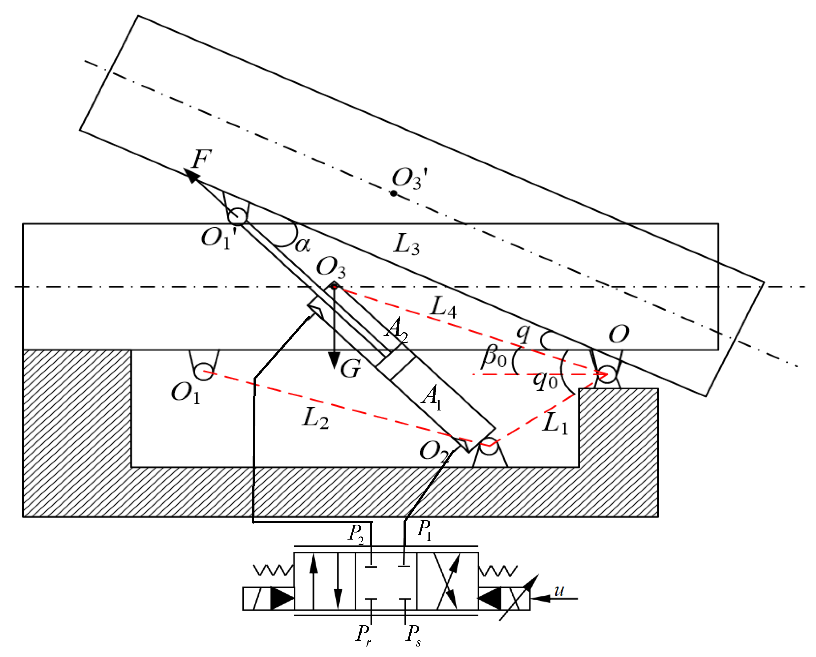
2. System Description

The hydraulic lifting system under study is presented in Figure 1. As shown in Figure 1, O stands for the gyration center; O₁ and O₂ denote the rotation centers of the upper and lower ears of the hydraulic cylinder, respectively; O₃ stands for the lifting system barycenter; q stands for the lifting arm rotary angle; G and F denote the force acting on the arm and the arm gravity, respectively. In addition, let OO₂ = L₁, O₁O₂ = L₂, OO₁ = L₃, OO₃ = L₄, $O_1{}^{\prime }{O}_2=L$, $\angle O_{1}O{O}_1{}^{\prime }=q$, ∠O₁OO₂ = q₀, ∠O₁OO₃ = β₀, and $\angle O{O}_1{}^{\prime }{O}_2=\alpha$.

The dynamics of the lifting system can be written as:

$$J\ddot{q}=\left(\frac{\partial x_p}{\partial q}\right)(P_1{A}_1-P_2{A}_2)-mg{L}_4\cos (q+{\beta }_0)-B\dot{q}-A_f{S}_f(\dot{q})+d_1(t)$$

(1)

where J and m stand for the rotary inertia and arm mass, respectively; P₁ and P₂ stand for the pressure values of two chambers of the hydraulic cylinder, respectively; A₁ and A₂ stand for the effective areas of two chambers in the hydraulic cylinder, respectively; A_f and S_f stand for the amplitude and approximated shape function of the Coulomb friction, respectively; B stands for the viscous friction coefficient; $d_1(t)$ stands for the unmodeled disturbances.

Defining the cylinder displacement as $x_p$ obtains:

$$\begin{array}{cc}\hfill x_p& =L-L_2\hfill \\ & =\sqrt{L_1^2+L_3^2-2L_1{L}_3\cos (q+q_0)}-L_2\hfill \end{array}$$

(2)

There exists:

$$\frac{\partial x_p}{\partial q}=\frac{L_1{L}_3\sin (q+q_0)}{\sqrt{L_1^2+L_3^2-2L_1{L}_3\cos (q+q_0)}}$$

(3)

Considering the oil compressibility, the pressure dynamics of the hydraulic actuator are written as [28]:

$$\begin{array}{l}{\dot{P}}_1=\frac{{\beta }_e}{V_1(q)}[-A_1\frac{\partial x_p}{\partial q}\dot{q}-C_t(P_1-P_2)+Q_1+d_{21}(t)]\\ {\dot{P}}_2=\frac{{\beta }_e}{V_2(q)}[A_2\frac{\partial x_p}{\partial q}\dot{q}+C_t(P_1-P_2)-Q_2-d_{22}(t)]\end{array}$$

(4)

where V₁ = V₀₁ + A₁x_s and V₂ = V₀₂ − A₂x_s stand for the volumes of the two chambers, respectively; V₀₁ and V₀₂ stand for the original volumes of the two chambers, respectively; ${\beta }_e$ stands for the effective oil bulk modulus; C_t stands for the internal leakage coefficient; Q₁ and Q₂ stand for the return flow and supplied flow of the hydraulic cylinder, respectively; d₂₁(t) and d₂₂(t) stand for the unmodeled disturbances.

Consequently, the flows Q₁ and Q₂ thus are modeled as [28]:

$$\begin{array}{l}{Q}_1=k_q{x}_v[s(x_v)\sqrt{P_s-P_1}+s(-x_v)\sqrt{P_1-P_r}]\\ Q_2=k_q{x}_v[s(x_v)\sqrt{P_2-P_r}+s(-x_v)\sqrt{P_s-P_2}]\end{array}$$

(5)

where k_q stands for the flow gain; $x_v$ stands for the valve spool displacement; P_r and P_s stand for the return pressure and supply pressure, respectively; s(*) is defined as:

$$s(*)=\{\begin{array}{ll}1,& \mathrm{if} \ast \ge 0\\ 0,& \mathrm{if} \ast <0\end{array}$$

(6)

Given that the compressibility flow is small and the valve window is configured and symmetrical, one obtains [28]:

$$P_s\approx P_1+P_2$$

(7)

Defining the load pressure $P_L=P_1-{\overline{A}}_c{P}_2$, where ${\overline{A}}_c=A_2/A_1$, it is easy to derive:

$$P_1=\frac{{\overline{A}}_c{P}_s+P_L}{1+{\overline{A}}_c}, P_2=\frac{P_s-P_L}{1+{\overline{A}}_c}$$

(8)

Defining the state variables $x=\left[x_1;x_2;x_3\right]=\left[q;\dot{q};A_1{P}_L/J\right]$, the system’s state-space form using (1)–(5) and (8) is:

$$\begin{array}{l}{\dot{x}}_1=x_2\\ {\dot{x}}_2=\frac{\partial x_p}{\partial x_1}{x}_3-\frac{m}{J}{g}_1(x_1)-\frac{B}{J}{x}_2-\frac{A_f}{J}{S}_f(x_2)+{\Delta }_1(t)\\ {\dot{x}}_3=\frac{{\beta }_e{k}_t}{J}{g}_2(x_v,x_3)\cdot x_v(u)-\frac{{\beta }_e}{J}{g}_3(x_1,x_2)-\frac{{\beta }_e{C}_t}{J}{g}_4(x_1,x_3)+{\Delta }_2(t)\end{array}$$

(9)

where

$$\begin{array}{l}{g}_1\left(x_1\right)=g{L}_{4}cos\left(x_1+{\beta }_0\right) \\ {\Delta }_1\left(t\right)=d_1\left(t\right)/J\\ {\Delta }_2\left(t\right)={\beta }_e\left(A_1{d}_{21}\left(t\right)/V_1+A_2{d}_{22}\left(t\right)/V_2\right)/J\end{array}$$

(10)

and

$$\begin{array}{l}{g}_2(x_v,x_3)=\frac{A_1{R}_1{}^{\prime }}{V_1}+\frac{A_2{R}_2{}^{\prime }}{V_2},\\ R_1{}^{\prime }=s(x_v)\sqrt{P_s-\frac{{\overline{A}}_c{P}_s+J{x}_3/A_1}{1+{\overline{A}}_c}}+s(-x_v)\sqrt{\frac{{\overline{A}}_c{P}_s+J{x}_3/A_1}{1+{\overline{A}}_c}-P_r},\\ R_2{}^{\prime }=s(x_v)\sqrt{\frac{P_s-J{x}_3/A_1}{1+{\overline{A}}_c}-P_r}+s(-x_v)\sqrt{P_s-\frac{P_s-J{x}_3/A_1}{1+{\overline{A}}_c}},\\ g_3(x_1,x_2)=\frac{\partial x_p}{\partial x_1}(\frac{A_1^2}{V_1}+\frac{A_2^2}{V_2})x_2, g_4(x_1,x_3)=(\frac{A_1}{V_1}+\frac{A_2}{V_2})\frac{({\overline{A}}_c-1)P_s+\frac{2J{x}_3}{A_1}}{1+{\overline{A}}_c}\end{array}$$

(11)

Omitting the valve dynamics, the valve spool displacement, $x_v$, can be modeled as a static mapping of the control input voltage, u, with a dead-zone [29]

$$x_v(u)=DZ(u)=\{\begin{array}{cc}{m}_{r}u-m_r{b}_r,& \mathrm{if} u\ge b_r\\ 0,& \mathrm{if} b_l<u<b_r\\ m_{l}u-m_l{b}_l,& \mathrm{if} u\le b_l\end{array}$$

(12)

where $DZ(u)$ stands for the valve dead-zone nonlinear function; $m_r>0$, $m_l>0$, $b_r\ge 0$, and $b_l\ge 0$ denote the unknown constants of the right slope, left slope, right break-point, and left break-point of the dead-zone, respectively. The characteristic of the valve dead-zone is given in Figure 2.

Assumption 1.

Although the valve dead-zone parameters are unknown, the maximum and minimum values of the left slope and right slope are known, i.e., $\overline{m}$ = max{$m_r$, $m_l$} and $\underset{\_}{m}$ = min{$m_r$, $m_l$}, where $\overline{m}$ and $\underset{\_}{m}$ are known positive constants.

Based on Assumption 1, Formula (12) can be reconstructed as:

$$x_v(u)=m(t)u+d(t)$$

(13)

in which

$$m(t)\triangleq \{\begin{array}{cc}{m}_l,& \mathrm{if} u\le 0\\ m_r,& \mathrm{if} u>0\end{array}$$

(14)

and

$$d(t)\triangleq \{\begin{array}{cc}-m_r{b}_r,& \mathrm{if} u\ge b_r\\ -m(t)u,& \mathrm{if} b_l<u<b_r\\ -m_l{b}_l,& \mathrm{if} u\le b_l\end{array}$$

(15)

It is worth noting that:

$$\frac{m(t)}{\underset{\_}{m}}=1+k(t)$$

(16)

where $k(t)$ stands for a positive bounded piecewise continuous function.

Taking the parametric uncertainties into consideration, defining the unknown parameter vector, $\theta =\left[{\theta }_1;{\theta }_2;{\theta }_3;{\theta }_4;{\theta }_5;{\theta }_6\right]=\left[\frac{m}{J};\frac{B}{J};\frac{A_f}{J};\frac{{\beta }_e{k}_t}{J};\frac{{\beta }_e}{J};\frac{{\beta }_e{C}_t}{J}\right]$. According to (9), (13) and (16) can be rewritten by:

$$\begin{array}{l}{\dot{x}}_1=x_2\\ {\dot{x}}_2=\frac{\partial x_p}{\partial x_1}{x}_3-{\theta }_1{g}_1(x_1)-{\theta }_2{x}_2-{\theta }_3{S}_f(x_2)+{\Delta }_1(t)\\ {\dot{x}}_3={\theta }_4{g}_2(x_v,x_3)u-{\theta }_5{g}_3(x_1,x_2)-{\theta }_6{g}_4(x_1,x_3)+{\overline{\Delta }}_2(t)\end{array}$$

(17)

in which ${\overline{\Delta }}_2(t)={\Delta }_2(t)+\underset{\_}{m}k(t)u+d(t)$.

Before developing the controller, the following assumptions were provided:

Assumption 2.

The desired trajectory $x_{1d}\in {ℂ}^3$ is bounded.

Assumption 3.

${\Delta }_1(t)$and${\overline{\Delta }}_2(t)$in (17) meet:

$$\left|{\Delta }_1(t)\right|\le {\delta }_1, \left|{\overline{\Delta }}_2(t)\right|\le {\delta }_2$$

(18)

where ${\delta }_i$ ($i=1,2$) are unknown positive constants. In addition, the set of parameters $\theta$ satisfies:

$$\theta \in {\Omega }_{\theta }\triangleq \left\{\theta :{\theta }_{\min }\le \theta \le {\theta }_{\max }\right\}$$

(19)

where ${\theta }_{\max }=[{\theta }_{1\max };{\theta }_{2\max };{\theta }_{3\max };{\theta }_{4\max };{\theta }_{5\max };{\theta }_{6\max }]$, ${\theta }_{\min }=[{\theta }_{1\min };{\theta }_{2\min };{\theta }_{3\min };{\theta }_{4\min };{\theta }_{5\min };{\theta }_{6\min }]$.

3. Controller Design

3.1. Discontinuous Mapping and Parameter Adaptive Law

Defining the estimation values of $\theta$ as $\widehat{\theta }$, and the estimation error $\tilde{\theta }=\widehat{\theta }-\theta$, the discontinuous mapping was designed as [30]:

$${\mathrm{Proj}}_{{\widehat{\theta }}_i}({•}_i)=\{\begin{array}{l}0,\hspace{1em}\mathrm{if} {\widehat{\theta }}_i={\theta }_{i\max } \mathrm{and} {•}_i>0\\ 0,\hspace{1em}\mathrm{if} {\widehat{\theta }}_i={\theta }_{i\min } \mathrm{and} {•}_i<0\\ {•}_i,\hspace{1em}\mathrm{otherwise}\end{array}$$

(20)

in which i = 1, 2, 3, 4, 5, and 6. The adopted updated law is set as:

$$\dot{\widehat{\mathit{\theta }}}={\mathrm{Proj}}_{\widehat{\mathit{\theta }}}(\mathsf{\Gamma }\mathit{\tau })\hspace{1em}\widehat{\mathit{\theta }}(0)\in {\mathsf{\Omega }}_{\mathit{\theta }}$$

(21)

where ${\mathrm{Proj}}_{\widehat{\mathit{\theta }}}(•)={[{\mathrm{Proj}}_{{\widehat{\theta }}_1}({•}_1),\dots ,{\mathrm{Proj}}_{{\widehat{\theta }}_6}({•}_6)]}^{\mathrm{T}}$; $\mathsf{\Gamma }\in {ℝ}^{6\times 6}$ denotes a positive diagonal matrix, for any adapted function $\mathit{\tau }$, the projection mapping (20) ensures [30]:

$$\widehat{\mathit{\theta }}\in {\Omega }_{\widehat{\mathit{\theta }}}=\{\widehat{\mathit{\theta }}:{\mathit{\theta }}_{\mathbf{min}}\le \widehat{\mathit{\theta }}\le {\mathit{\theta }}_{\mathbf{max}}\}$$

(22)

$${\tilde{\mathit{\theta }}}^{{\rm T}}[{\mathsf{\Gamma }}^{-1}{\mathrm{Proj}}_{\widehat{\mathit{\theta }}}(\mathsf{\Gamma }\mathit{\tau })-\mathit{\tau }]\le 0, \forall \mathit{\tau }$$

(23)

3.2. Disturbance Observer Design

To realize the observation of matching and mismatching disturbances in (17), the disturbance observer should be designed first. We defined the disturbances ${\Delta }_1(t)$ and ${\overline{\Delta }}_2(t)$ as the extended states $x_{e1}$ and $x_{e2}$, and the variables $H_1(t)={\dot{x}}_{ei}$ for i = 1, 2. In addition, we assumed the functions $H_1(t)$ and $H_2(t)$ were unknown bounded. Hence, based on (17), two extended state disturbance observers were constructed as:

$$\{\begin{array}{l}{\dot{\widehat{x}}}_1={\widehat{x}}_2+3{\omega }_{o1}(x_1-{\widehat{x}}_1)\\ {\dot{\widehat{x}}}_2=\frac{\partial x_p}{\partial x_1}{x}_3+{\widehat{\mathit{\theta }}}^T{\mathit{\phi }}_2+{\widehat{x}}_{e1}+3{\omega }_{o1}^2(x_1-{\widehat{x}}_1)\\ {\dot{\widehat{x}}}_{e1}={\omega }_{o1}^3(x_1-{\widehat{x}}_1)\end{array}$$

(24)

$$\{\begin{array}{l}{\dot{\widehat{x}}}_3={\widehat{\mathit{\theta }}}^T{\mathit{\phi }}_3+{\widehat{x}}_{e2}+2{\omega }_{o2}(x_3-{\widehat{x}}_3)\\ {\dot{\widehat{x}}}_{e2}={\omega }_{o2}^2(x_3-{\widehat{x}}_3)\end{array}$$

(25)

where ${\mathit{\phi }}_2=\left[-g_1\left(x_1\right);-x_2;-S_f\left(x_2\right);0;0;0\right]$; ${\mathit{\phi }}_3=\left[0;0;0;g_2\left(x_v,x_3\right)u;-g_3\left(x_1,x_2\right);-g_4\left(x_1,x_3\right)\right]$; ${\omega }_{o1}$ and ${\omega }_{o2}$ denote the adjustable parameters of observers (24) and (25); $\widehat{·}$ denotes the estimation of $·$, and the estimation error of $·$ is defined as $\widetilde{·}=\widehat{·}-·$ throughout the paper.

Considering the existence of the parametric uncertainties, $\tilde{\theta }$, and the disturbances, ${\Delta }_1(t)$ and ${\overline{\Delta }}_2(t)$, the following two constructed forms of $x_{e1}$ and $x_{e2}$ are given as:

(1) Define $x_{e1}={\Delta }_1(t)$ and $x_{e2}={\overline{\Delta }}_2(t)$; then, (17) is rewritten as:

$$\{\begin{array}{l}{\dot{x}}_1=x_2\\ {\dot{x}}_2=\frac{\partial x_p}{\partial x_1}{x}_3+{\widehat{\mathit{\theta }}}^T{\mathit{\phi }}_2-{\tilde{\mathit{\theta }}}^T{\mathit{\phi }}_2+x_{e1}\\ {\dot{x}}_{e1}=H_1(t)\end{array}$$

(26)

$$\{\begin{array}{l}{\dot{x}}_3={\widehat{\mathit{\theta }}}^T{\mathit{\phi }}_3-{\tilde{\mathit{\theta }}}^T{\mathit{\phi }}_3+x_{e2}\\ {\dot{x}}_{e2}=H_2(t)\end{array}$$

(27)

Defining $\eta ={\left[{\eta }_1,{\eta }_2,{\eta }_3\right]}^T={[{\tilde{x}}_1, {\tilde{x}}_2/{\omega }_{o1}, {\tilde{x}}_{e1}/{\omega }_{o1}^2]}^T$, $\chi ={\left[{\chi }_1,{\chi }_2\right]}^T={[{\tilde{x}}_3, {\tilde{x}}_{e2}/{\omega }_{o2}]}^T$, and based on (24)–(27), the dynamics of the designed observers are presented as:

$$\{\begin{array}{l}\dot{\mathit{\eta }}={\omega }_{o1}{\mathit{A}}_1\mathit{\eta }-{\mathit{B}}_1\frac{{\tilde{\mathit{\theta }}}^T{\mathit{\phi }}_2}{{\omega }_{o1}}+{\mathit{B}}_2\frac{H_1(t)}{{\omega }_{o1}^2}\\ \dot{\mathit{\chi }}={\omega }_{o2}{\mathit{A}}_2\mathit{\chi }-{\mathit{B}}_3{\tilde{\mathit{\theta }}}^T{\mathit{\phi }}_3+{\mathit{B}}_4\frac{H_2(t)}{{\omega }_{o2}}\end{array}$$

(28)

in which B₁ = [0, 1, 0]^T, B₂ = [0, 0, 1]^T, B₃ = [1, 0]^T, B₄ = [0, 1]^T and

$${\mathit{A}}_1=\left[\begin{array}{ccc}-3& 1& 0\\ -3& 0& 1\\ -1& 0& 0\end{array}\right],{\mathit{A}}_2=\left[\begin{array}{cc}-2& 1\\ -1& 0\end{array}\right]\circ$$

(29)

(2) Define $x_{e1}={\Delta }_1(t)-{\tilde{\mathit{\theta }}}^T{\mathit{\phi }}_2$ and $x_{e2}={\overline{\Delta }}_2(t)-{\tilde{\mathit{\theta }}}^T{\mathit{\phi }}_3$; then, (17) is rewritten as:

$$\{\begin{array}{l}{\dot{x}}_1=x_2\\ {\dot{x}}_2=\frac{\partial x_p}{\partial x_1}{x}_3+{\widehat{\mathit{\theta }}}^T{\mathit{\phi }}_2+x_{e1}\\ {\dot{x}}_{e1}=H_1(t)\end{array}$$

(30)

$$\{\begin{array}{l}{\dot{x}}_3={\widehat{\mathit{\theta }}}^T{\mathit{\phi }}_3+x_{e2}\\ {\dot{x}}_{e2}=H_2(t)\end{array}$$

(31)

Based on (24), (25), (30) and (31), the dynamics of the designed observers are presented as:

$$\{\begin{array}{l}\dot{\mathit{\eta }}={\omega }_{o1}{\mathit{A}}_1\mathit{\eta }+{\mathit{B}}_2\frac{H_1(t)}{{\omega }_{o1}^2}\\ \dot{\mathit{\chi }}={\omega }_{o2}{\mathit{A}}_2\mathit{\chi }+{\mathit{B}}_4\frac{H_2(t)}{{\omega }_{o2}}\end{array}$$

(32)

Since the matrices ${\mathit{A}}_1$ and ${\mathit{A}}_2$ are Hurwitz, there always exist positive definite matrices ${\mathit{P}}_1$ and ${\mathit{P}}_2$ meeting ${\mathit{A}}_1^T{\mathit{P}}_1+{\mathit{P}}_1{\mathit{A}}_1=-\mathit{I},$ and ${\mathit{A}}_2^T{\mathit{P}}_2+{\mathit{P}}_2{\mathit{A}}_2=-\mathit{I}$, where $\mathit{I}$ denotes the unit matrix. Hence, one has:

$${\mathit{P}}_1=\left[\begin{array}{ccc}1& -\frac{1}{2}& -1\\ -\frac{1}{2}& 1& -\frac{1}{2}\\ -1& -\frac{1}{2}& 4\end{array}\right],{\mathit{P}}_2=\left[\begin{array}{cc}\frac{1}{2}& -\frac{1}{2}\\ -\frac{1}{2}& \frac{3}{2}\end{array}\right]\circ$$

(33)

3.3. Controller Design

In this section, the backstepping method [31] was utilized to develop the controller. The details are as follows:

Step 1: Several error variables were designed as below:

$$\begin{array}{l}{z}_2={\dot{z}}_1+k_1{z}_1=x_2-{\alpha }_1,\\ {\alpha }_1={\dot{x}}_{1d}-k_1{z}_1, z_3=x_3-{\alpha }_2\end{array}$$

(34)

where $z_1=x_1-x_{1d}$ denotes the tracking error; $k_1$ stands for the feedback gain.

According to (17) and (34), and differentiating $z_2$, there is:

$$\begin{array}{cc}\hfill {\dot{z}}_2& ={\dot{x}}_2-{\dot{\alpha }}_1\hfill \\ & =\frac{\partial x_p}{\partial x_1}(z_3+{\alpha }_2)+{\widehat{\mathit{\theta }}}^T{\mathit{\phi }}_2-{\tilde{\mathit{\theta }}}^T{\mathit{\phi }}_2+{\Delta }_1(t)-{\dot{\alpha }}_1\hfill \end{array}$$

(35)

From (35), the virtual control ${\alpha }_2$ is constructed as:

$$\begin{array}{l}{\alpha }_2={\alpha }_{2a}+{\alpha }_{2s},\\ {\alpha }_{2a}={\left(\frac{\partial x_p}{\partial x_1}\right)}^{-1}(-{\widehat{\mathit{\theta }}}^T{\mathit{\phi }}_2+{\dot{\alpha }}_1-{\widehat{x}}_{e1}),\\ {\alpha }_{2s}=-{\left(\frac{\partial x_p}{\partial x_1}\right)}^{-1}{k}_2{z}_2\end{array}$$

(36)

where $k_2$ stands for the feedback gain.

Putting (36) into (35), one obtains:

$${\dot{z}}_2=\frac{\partial x_p}{\partial x_1}{z}_3-k_2{z}_2+{\tilde{x}}_{e1}+{\Delta }_1(t)-{\tilde{\mathit{\theta }}}^T{\mathit{\phi }}_2-x_{e1}$$

(37)

Step 2: On the basis of (17) and (34), and differentiating z₃, there is:

$$\begin{array}{cc}\hfill {\dot{z}}_3& ={\dot{x}}_3-{\dot{\alpha }}_2\hfill \\ & ={\widehat{\theta }}_4{g}_2(x_v,x_3)u-{\widehat{\theta }}_5{g}_3(x_1,x_2)-{\widehat{\theta }}_6{g}_4(x_1,x_3)-{\tilde{\mathit{\theta }}}^T{\mathit{\phi }}_3+{\overline{\Delta }}_2(t)-{\dot{\alpha }}_2\hfill \end{array}$$

(38)

Given that ${\dot{\alpha }}_2$ contains the incalculable part, it has:

$$\begin{array}{l}{\dot{\alpha }}_2(t,x_1,x_2,\widehat{\mathit{\theta }},{\widehat{x}}_{e1})={\dot{\alpha }}_{2c}+{\dot{\alpha }}_{2u},\\ {\dot{\alpha }}_{2c}=\frac{\partial {\alpha }_2}{\partial t}+\frac{\partial {\alpha }_2}{\partial x_1}{x}_2+\frac{\partial {\alpha }_2}{\partial x_2}(\frac{\partial x_p}{\partial x_1}{x}_3+{\widehat{\mathit{\theta }}}^T{\mathit{\phi }}_2+{\widehat{x}}_{e1})+\frac{\partial {\alpha }_2}{\partial \widehat{\mathit{\theta }}}\dot{\widehat{\mathit{\theta }}}+\frac{\partial {\alpha }_2}{\partial x_{e1}}{\dot{\widehat{x}}}_{e1},\\ {\dot{\alpha }}_{2u}=\frac{\partial {\alpha }_2}{\partial x_2}({\Delta }_1(t)-{\tilde{\mathit{\theta }}}^T{\mathit{\phi }}_2-x_{e1}+{\tilde{x}}_{e1})\end{array}$$

(39)

in which ${\dot{\alpha }}_{2c}$ stands for the calculable part; ${\dot{\alpha }}_{2u}$ stands for the incalculable part.

Hence, the controller input, u, is designed as below:

$$\begin{array}{l}u=u_a+u_s,\\ u_a=\frac{1}{{\widehat{\theta }}_4{g}_2(x_v,x_3)}[{\widehat{\theta }}_5{g}_3(x_1,x_2)+{\widehat{\theta }}_6{g}_4(x_1,x_3)+{\dot{\alpha }}_{2c}-{\widehat{x}}_{e2}],\\ u_s=-\frac{1}{{\widehat{\theta }}_4{g}_2(x_v,x_3)}{k}_3{z}_3\end{array}$$

(40)

where $k_3$ stands for the feedback gain.

Putting (40) into (38), one obtains:

$${\dot{z}}_3=-k_3{z}_3+{\tilde{x}}_{e2}+{\overline{\Delta }}_2(t)-{\tilde{\mathit{\theta }}}^T{\mathit{\phi }}_3-x_{e2}-{\dot{\alpha }}_{2u}$$

(41)

3.4. Stability Analysis

The main results of this paper are provided below.

Theorem 1.

If the uncertain nonlinearities are constants (i.e.,), with Assumptions 1–3, the control law (40), choosing the adaption function $\mathit{\tau }$ as:

$$\mathit{\tau }=a_2{\mathit{\phi }}_2{z}_2+a_3({\mathit{\phi }}_3-\frac{\partial {\alpha }_2}{\partial x_2}{\mathit{\phi }}_2)z_3+c_2{\mathit{\eta }}^T{\mathit{P}}_1{\mathit{B}}_1\frac{{\mathit{\phi }}_2}{{\omega }_{o1}}+c_3{\mathit{\chi }}^T{\mathit{P}}_2{\mathit{B}}_3{\mathit{\phi }}_3$$

(42)

and picking up the proper control parameters, $k_1$, $k_2$, and $k_3$, and the positive coordinating parameters $a_j$ and $c_j$ for j = 2, 3, such that the matrix Λ defined below is positive definite:

$$\mathsf{\Lambda }=\left[\begin{array}{ccc}{\mathsf{\Lambda }}_1& 0& {\mathsf{\Lambda }}_3\\ 0& {\varpi }_1& 0\\ {\mathsf{\Lambda }}_3^T& 0& {\mathsf{\Lambda }}_2\end{array}\right]$$

(43)

in which $0$ denotes the zero vector and

$${\mathsf{\Lambda }}_1=\left[\begin{array}{ccc}{k}_1& -\frac{1}{2}& 0\\ -\frac{1}{2}& k_2{a}_2& -\frac{a_2}{2}\frac{\partial x_p}{\partial x_1}\\ 0& -\frac{a_2}{2}\frac{\partial x_p}{\partial x_1}& k_3{a}_3\end{array}\right], {\mathsf{\Lambda }}_2=\left[\begin{array}{cccc}{\varpi }_1& 0& 0& 0\\ 0& {\varpi }_1& 0& 0\\ 0& 0& {\varpi }_2& 0\\ 0& 0& 0& {\varpi }_2\end{array}\right],{\mathsf{\Lambda }}_3=\left[\begin{array}{cccc}0& 0& 0& 0\\ 0& -\frac{{\gamma }_1}{2}& 0& 0\\ 0& -\frac{{\gamma }_2}{2}& 0& -\frac{{\gamma }_3}{2}\end{array}\right]$$

(44)

in which

$$\begin{array}{l}{\varpi }_1=\frac{c_2({\omega }_{o1}-1)}{2}, {\varpi }_2=\frac{c_3({\omega }_{o2}-1)}{2},\\ {\gamma }_1=a_2{\omega }_{o1}^2, {\gamma }_2=a_3{\omega }_{o1}^2\left|\frac{\partial {\alpha }_2}{\partial x_2}\right|, {\gamma }_3=a_3{\omega }_{o2}\end{array}$$

(45)

then it can be concluded that all the closed-loop signals are bounded, and asymptotic tracking performance is also realized, i.e., $z_1\to 0$ as $t\to +\infty$.

Proof of Theorem 1.

For this case, define $x_{e1}={\Delta }_1(t)$ and $x_{e2}={\overline{\Delta }}_2(t)$, and choose a Lyapunov function as:

$$V_1=\frac{1}{2}{z}_1^2+\frac{1}{2}{a}_2{z}_2^2+\frac{1}{2}{a}_3{z}_3^2+\frac{1}{2}{c}_2{\mathit{\eta }}^T{\mathit{P}}_1\mathit{\eta }+\frac{1}{2}{c}_3{\mathit{\chi }}^T{\mathit{P}}_2\mathit{\chi }+\frac{1}{2}{\tilde{\mathit{\theta }}}^T{\mathsf{\Gamma }}^{-1}\tilde{\mathit{\theta }}$$

(46)

According to (28), (34), (37) and (41), there is:

$$\begin{array}{ccc}\hfill {\dot{V}}_1& =& z_1{\dot{z}}_1+a_2{z}_2{\dot{z}}_2+a_3{z}_3{\dot{z}}_3+\frac{1}{2}{c}_2{\dot{\mathit{\eta }}}^T{\mathit{P}}_1\mathit{\eta }+\frac{1}{2}{c}_2{\mathit{\eta }}^T{\mathit{P}}_1\dot{\mathit{\eta }}\hfill \\ & & +\frac{1}{2}{c}_3{\dot{\mathit{\chi }}}^T{\mathit{P}}_2\mathit{\chi }+\frac{1}{2}{c}_3{\mathit{\chi }}^T{\mathit{P}}_2\dot{\mathit{\chi }}+{\tilde{\mathit{\theta }}}^T{\mathsf{\Gamma }}^{-1}\dot{\widehat{\mathit{\theta }}}\hfill \\ & =& z_1(z_2-k_1{z}_1)+a_2{z}_2(\frac{\partial x_p}{\partial x_1}{z}_3-k_2{z}_2+{\tilde{x}}_{e1}-{\tilde{\mathit{\theta }}}^T{\mathit{\phi }}_2)+a_3{z}_3[-k_3{z}_3+{\tilde{x}}_{e2}\hfill \\ & & -{\tilde{\mathit{\theta }}}^T{\mathit{\phi }}_3-\frac{\partial {\alpha }_2}{\partial x_2}(-{\tilde{\mathit{\theta }}}^T{\mathit{\phi }}_2+{\tilde{x}}_{e1})]-\frac{1}{2}{c}_2{\omega }_{o1}{\Vert \mathit{\eta }\Vert }^2-c_2{\mathit{\eta }}^T{\mathit{P}}_1{\mathit{B}}_1\frac{{\tilde{\mathit{\theta }}}^T{\mathit{\phi }}_2}{{\omega }_{o1}}\hfill \\ & & -\frac{1}{2}{c}_3{\omega }_{o2}{\Vert \mathit{\chi }\Vert }^2-c_3{\mathit{\chi }}^T{\mathit{P}}_2{\mathit{B}}_3{\tilde{\mathit{\theta }}}^T{\mathit{\phi }}_3+{\tilde{\mathit{\theta }}}^T{\mathsf{\Gamma }}^{-1}\dot{\widehat{\mathit{\theta }}}\hfill \end{array}$$

(47)

Putting (42) into (47), it has:

$$\begin{array}{cc}\hfill {\dot{V}}_1\le & -k_1{z}_1^2+\left|z_1\right|\left|z_2\right|+a_2\frac{\partial x_p}{\partial x_1}\left|z_2\right|\left|z_3\right|-k_2{a}_2{z}_2^2+a_2{\omega }_{o1}^2\left|z_2\right|\left|{\eta }_3\right|\hfill \\ & -k_3{a}_3{z}_3^2+a_3{\omega }_{o2}\left|z_3\right|\left|{\chi }_2\right|+a_3{\omega }_{o1}^2\left|\frac{\partial {\alpha }_2}{\partial x_2}\right|\left|z_3\right|\left|{\eta }_3\right|-\frac{1}{2}{c}_2({\omega }_{o1}-1){\Vert \mathit{\eta }\Vert }^2\hfill \\ & -\frac{1}{2}{c}_3({\omega }_{o2}-1){\Vert \mathit{\chi }\Vert }^2-\frac{1}{2}{c}_2{\Vert \mathit{\eta }\Vert }^2-\frac{1}{2}{c}_3{\Vert \mathit{\chi }\Vert }^2\hfill \end{array}$$

(48)

This results in:

$$\begin{array}{cc}\hfill {\dot{V}}_1& \le -{\mathit{Z}}^T\mathsf{\Lambda }\mathit{Z}\hfill \\ & \le -{\lambda }_{\min }(\mathsf{\Lambda })({\mathbf{z}}^T\mathbf{z}+{\mathit{\eta }}_a^T{\mathit{\eta }}_a+{\mathit{\chi }}_a^T{\mathit{\chi }}_a)\triangleq -M\hfill \end{array}$$

(49)

where $\mathit{Z}={\left[({\mathit{z}}^T,{\mathit{\eta }}_a{}^T,{\mathit{\chi }}_a{}^T\right]}^T$, $\mathit{z}={\left[\left|z_1\right|, \left|z_2\right|, \left|z_3\right|\right]}^T$, ${\mathit{\eta }}_a={\left[\left|{\eta }_1\right|, \left|{\eta }_2\right|, \left|{\eta }_3\right|\right]}^T$, ${\mathit{\chi }}_a={\left[\left|{\chi }_1\right|, \left|{\chi }_2\right|\right]}^T$, and ${\lambda }_{\min }(\mathsf{\Lambda })$ denotes the minimum eigenvalue of the matrix $\mathsf{\Lambda }$.

Hence, $V_1\in L_{\infty }$, $M\in L_2$, and the boundness of all the system’s signals holds. Based on error dynamics, the time derivative of $M$ is bounded as well. Thus, it is concluded that $M$ is uniformly continuous. Using the Barbalat’s lemma [31], $M\to 0$ as $t\to \infty$. Consequently, the asymptotic stability of the closed-loop system can be ensured, i.e., the tracking error converges to zero asymptotically. As a result, Theorem 1 holds.  □

Theorem 2.

If the unknown nonlinearities are time-varying (i.e., $H_1(t)\ne 0$ and $H_2(t)\ne 0$), with Assumptions 1–3 and the control law (40), by picking up the proper control parameters, $k_1$, $k_2$, and $k_3$, then it can be concluded that all the closed-loop signals are uniformly bounded.

Proof of Theorem 2.

For this case, define $x_{e1}={\Delta }_1(t)-{\tilde{\mathit{\theta }}}^T{\mathit{\phi }}_2$ and $x_{e2}={\overline{\Delta }}_2(t)-{\tilde{\mathit{\theta }}}^T{\mathit{\phi }}_3$, and choose a Lyapunov function as:

$$V_2=\frac{1}{2}{z}_1^2+\frac{1}{2}{a}_2{z}_2^2+\frac{1}{2}{a}_3{z}_3^2+\frac{1}{2}{c}_2{\mathit{\eta }}^T{\mathit{P}}_1\mathit{\eta }+\frac{1}{2}{c}_3{\mathit{\chi }}^T{\mathit{P}}_2\mathit{\chi }$$

(50)

According to (32), (34), (37) and (41), there is:

$$\begin{array}{cc}\hfill {\dot{V}}_2=& z_1(z_2-k_1{z}_1)+a_2{z}_2(\frac{\partial x_p}{\partial x_1}{z}_3-k_2{z}_2+{\tilde{x}}_{e1})+a_3{z}_3(-k_3{z}_3+{\tilde{x}}_{e2}-\frac{\partial {\alpha }_2}{\partial x_2}{\tilde{x}}_{e1})\hfill \\ & -\frac{1}{2}{c}_2{\omega }_{o1}{\Vert \mathit{\eta }\Vert }^2+c_2{\mathit{\eta }}^T{\mathit{P}}_1{\mathit{B}}_2\frac{H_1(t)}{{\omega }_{o1}^2}-\frac{1}{2}{c}_3{\omega }_{o2}{\Vert \mathit{\chi }\Vert }^2+c_3{\mathit{\chi }}^T{\mathit{P}}_2{\mathit{B}}_4\frac{H_2(t)}{{\omega }_{o2}}\hfill \end{array}$$

(51)

One has:

$$\begin{array}{ccc}\hfill {\dot{V}}_2& \le & -k_1{z}_1^2+\left|z_1\right|\left|z_2\right|+a_2\frac{\partial x_p}{\partial x_1}\left|z_2\right|\left|z_3\right|-k_2{a}_2{z}_2^2+a_2{\omega }_{o1}^2\left|z_2\right|\left|{\eta }_3\right|\hfill \\ & & -k_3{a}_3{z}_3^2+a_3{\omega }_{o2}\left|z_3\right|\left|{\chi }_2\right|+a_3{\omega }_{o1}^2\left|\frac{\partial {\alpha }_2}{\partial x_2}\right|\left|z_3\right|\left|{\eta }_3\right|-\frac{1}{2}{c}_2({\omega }_{o1}-1){\Vert \mathit{\eta }\Vert }^2\hfill \\ & & -\frac{1}{2}{c}_2{\Vert \mathit{\eta }\Vert }^2+c_2\Vert \mathit{\eta }\Vert \frac{\Vert {\mathit{P}}_1{\mathit{B}}_2\Vert {\left|H_1(t)\right|}_{\max }}{{\omega }_{o1}^2}-\frac{1}{2}{c}_3({\omega }_{o2}-1){\Vert \mathit{\chi }\Vert }^2-\frac{1}{2}{c}_3{\Vert \mathit{\chi }\Vert }^2\hfill \\ & & +c_3\Vert \mathit{\chi }\Vert \frac{\Vert {\mathit{P}}_2{\mathit{B}}_4\Vert {\left|H_2(t)\right|}_{\max }}{{\omega }_{o2}}\hfill \\ & \le & -{\mathit{Z}}^T\mathsf{\Lambda }\mathit{Z}+\zeta \hfill \end{array}$$

(52)

in which

$$\zeta =\frac{1}{2}{c}_2{(\frac{\Vert {\mathit{P}}_1{\mathit{B}}_1\Vert {\left|H_1(t)\right|}_{\max }}{{\omega }_{o1}^2})}^2+\frac{1}{2}{c}_3{(\frac{\Vert {\mathit{P}}_2{\mathit{B}}_4\Vert {\left|H_2(t)\right|}_{\max }}{{\omega }_{o2}})}^2$$

(53)

This results in:

$$\begin{array}{cc}\hfill {\dot{V}}_2& \le -{\lambda }_{\min }(\mathsf{\Lambda })(|\left|\mathbf{z}\right|{|}^2+\left|\right|\mathit{\eta }|{|}^2+|\left|\mathit{\chi }\right|{|}^2)+\zeta \hfill \\ & \le -{\lambda }_{\min }(\mathsf{\Lambda })[{\lambda }_1(z_1^2+a_2{z}_2^2+a_3{z}_3^2)+\frac{1}{c_2{\lambda }_{\max }({\mathit{P}}_1)}{c}_2{\mathit{\eta }}^T{\mathit{P}}_1\mathit{\eta }+\frac{1}{c_3{\lambda }_{\max }({\mathit{P}}_2)}{c}_3{\mathit{\chi }}^T{\mathit{P}}_2\mathit{\chi }]+\zeta \hfill \\ & \le -{\lambda }_2{V}_2+\zeta \hfill \end{array}$$

(54)

where ${\lambda }_1=min\left\{1, 1/a_2, 1/a_3\right\}$, ${\lambda }_2=2{\lambda }_{min}\left(\Lambda \right)min\left\{{\lambda }_1,1/\left(c_2{\lambda }_{max}\left(P_1\right)\right), 1/\left(c_3{\lambda }_{max}\left(P_2\right)\right)\right\}$, and ${\lambda }_{\max }(·)$ and ${\lambda }_{\min }(·)$ denote the maximum and minimum eigenvalues of the matrix $·$, respectively.

Hence, using the comparison Lemma [31], it is easy to obtain:

$$V_2(t)\le V_2(0)e^{-{\lambda }_{2}t}+\frac{\zeta }{{\lambda }_2}(1-e^{-{\lambda }_{2}t})$$

(55)

Consequently, the uniformly ultimately bounded stability of the closed-loop system can be guaranteed, i.e., the tracking error is bounded, and all the system’s signals are bounded. Thus, Theorem 2 holds.  □

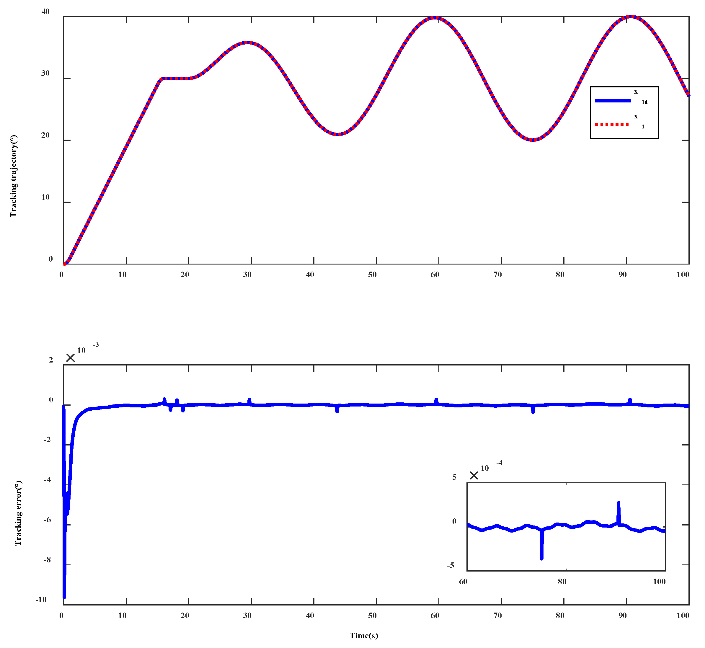
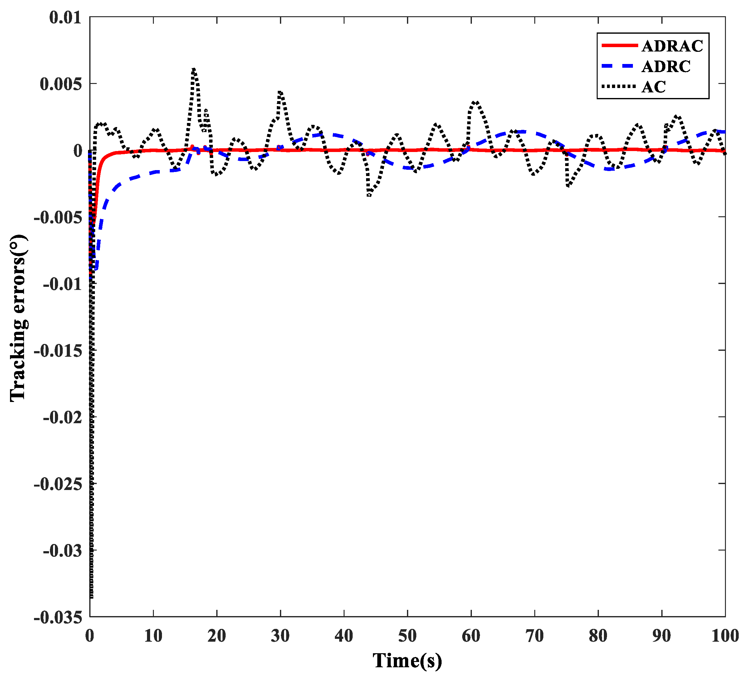
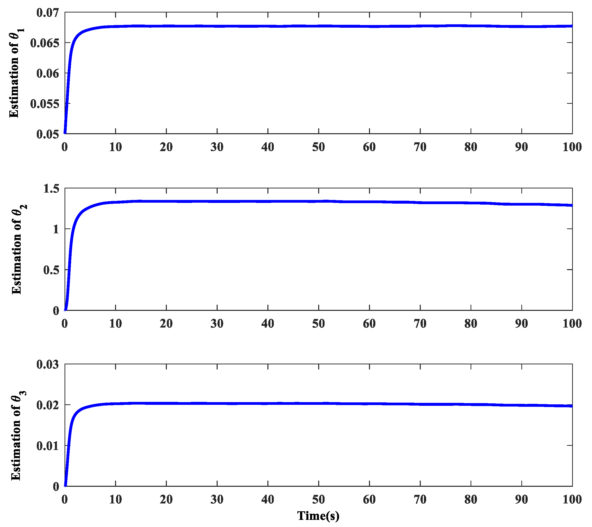
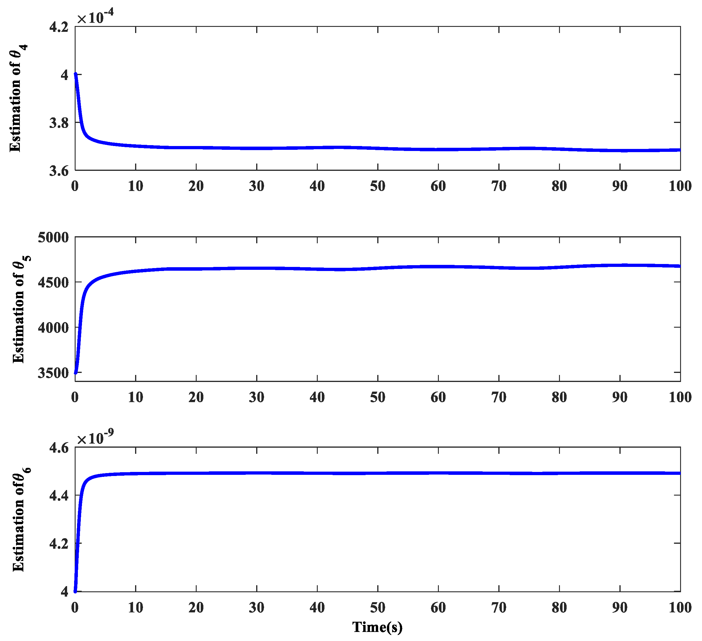
4. Simulation Results

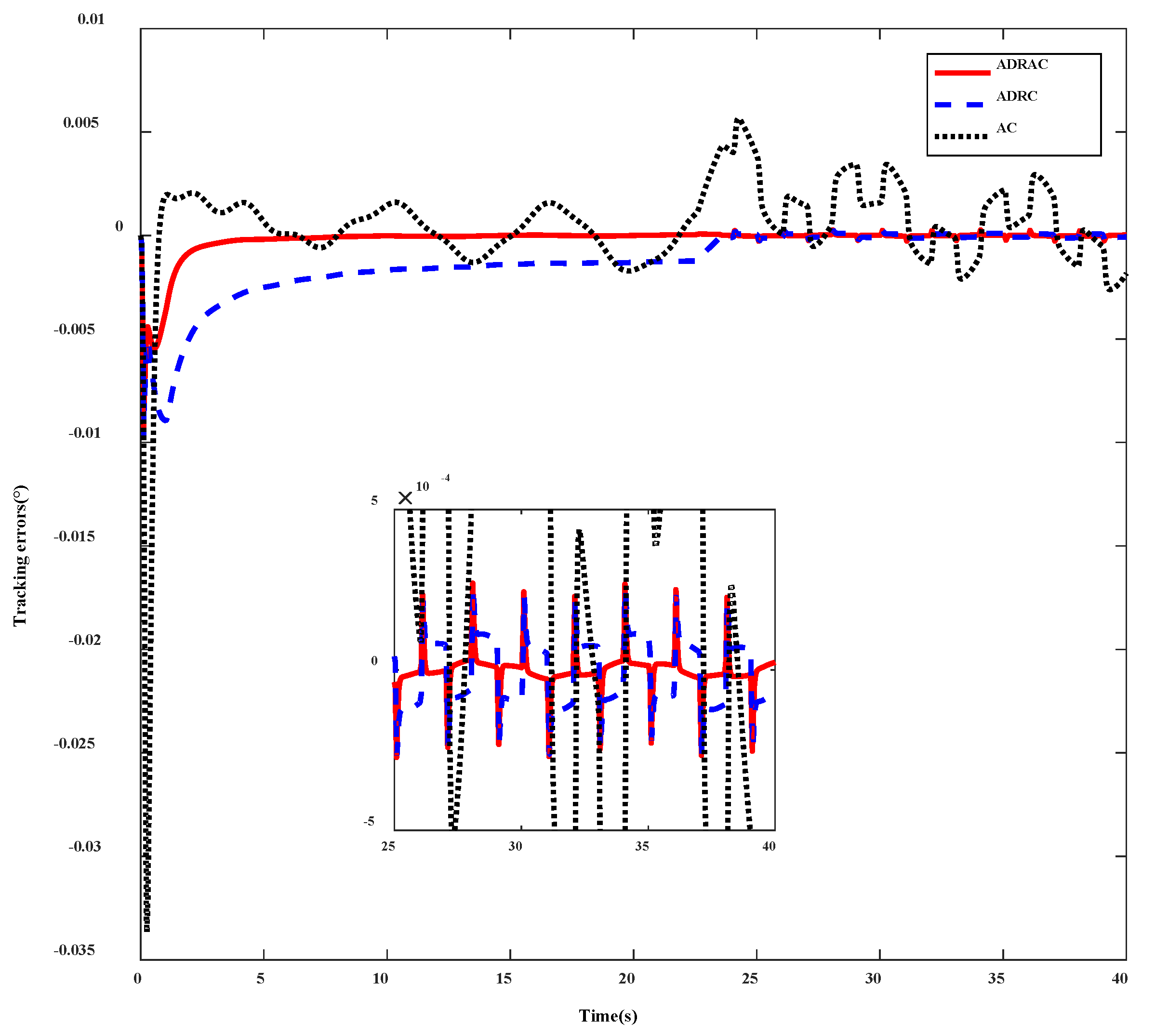
The physical parameters of the hydraulic lifting system are collected in

Table 1. Physical parameters of the hydraulic lifting system.

Parameter	Value	Parameter	Value
m (kg)	10,000	$B(\mathrm{N}\cdot \mathrm{m}\cdot \mathrm{s}/\mathrm{rad}$)	2.5 × 105
$J (\mathrm{kg}\cdot {\mathrm{m}}^2$)	1.5 × 105	$A_f (\mathrm{N}\cdot \mathrm{m}$)	3 × 103
Ps (Pa)	2.1 × 106	$k_t({\mathrm{m}}^4/(\mathrm{s}\cdot \mathrm{V}\cdot \sqrt{\mathrm{N}})$)	7.937× 10−8
Pr (Pa)	0	${\beta }_e$ (Pa)	7 × 108
A1 (m2)	3.14 × 10−2	$C_t ({\mathrm{m}}^5/(\mathrm{s}\cdot \mathrm{N})$)	9.6 × 10−13
A2 (m2)	1.6 × 10−2	L1 (m)	1.6
V01 (m3)	3.1416 × 10−4	L2 (m)	2
V02 (m3)	3.04 × 10−2	L3 (m)	3.5
g (m/s2)	9.8	L4 (m)	3
$q_0$ (rad)	0.2648	${\beta }_0$ (rad)	0.2618

. The function was set as $S_f(x_2)=2\arctan (900x_2)/\pi$, and the disturbances were set as $d_1\left(t\right)=50000sin\left(t\right)N·m$, d₂₁(t) = 5 × 10⁻⁵ sin (πt) m³/s, d₂₂(t) = −5 × 10⁻⁵ sin (πt) m³/s. The valve dead-zone nonlinear function was set as:

$$x_v(u)=DZ(u)=\{\begin{array}{cc}u-1,& \mathrm{if} u\ge 1\\ 0,& \mathrm{if} -1<u<1\\ u+1,& \mathrm{if} u\le -1\end{array}$$

(56)

where $m_r=1$, $m_l=1$, $b_r=1$, and $b_l=1$. The sample time was set as 0.5 ms.

Three controllers were compared to verify the validity of the developed controller.

(1)

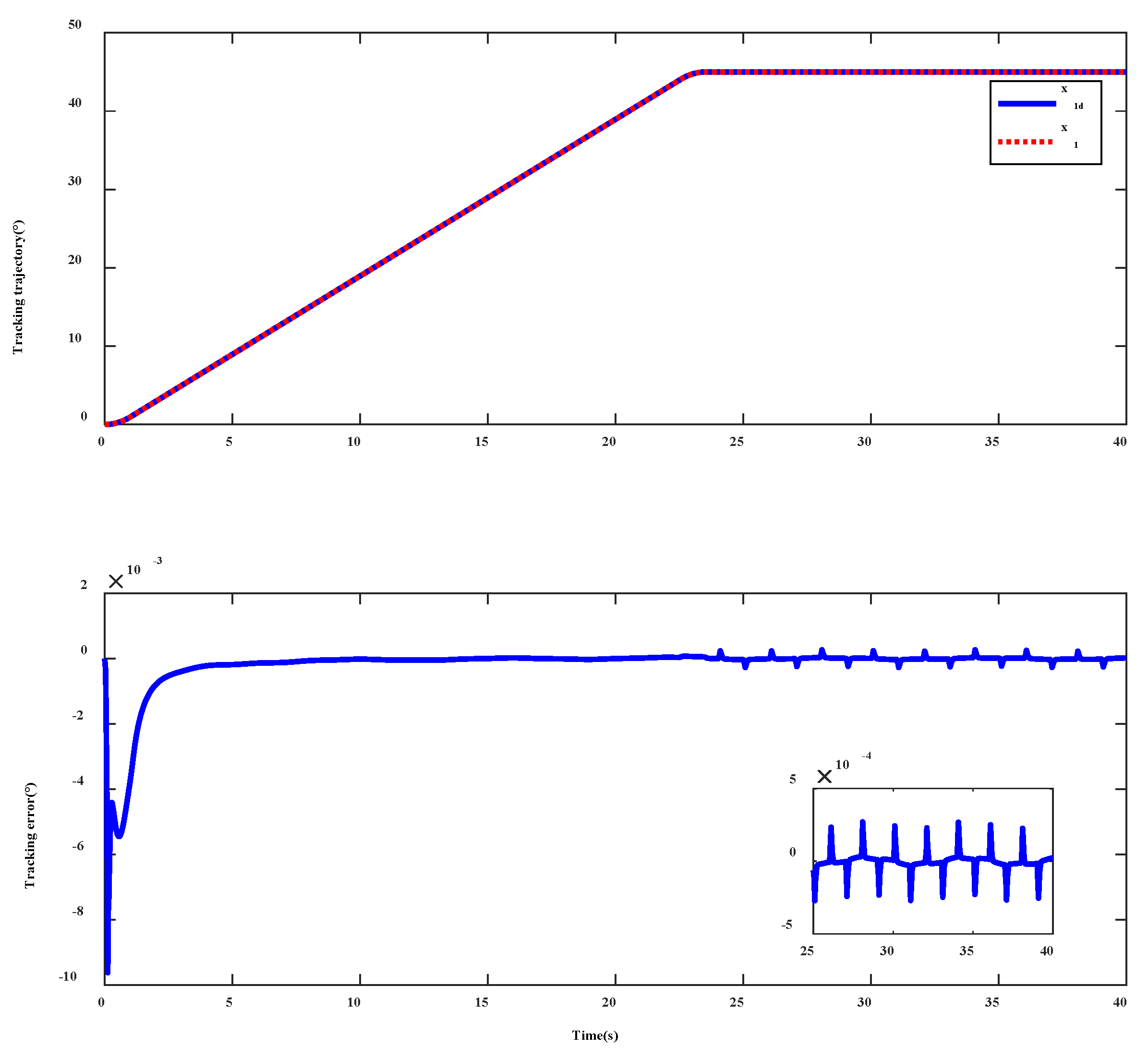
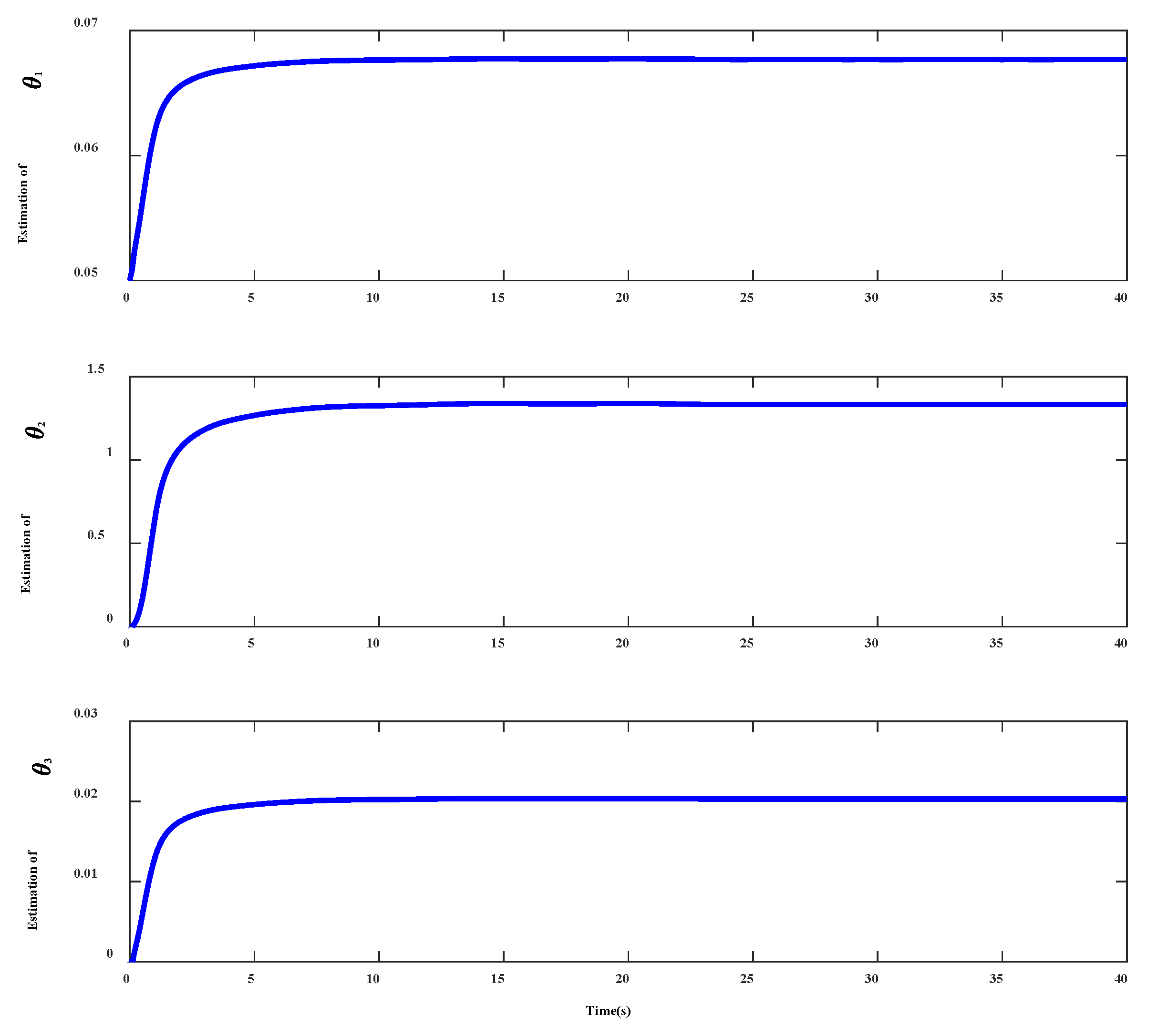
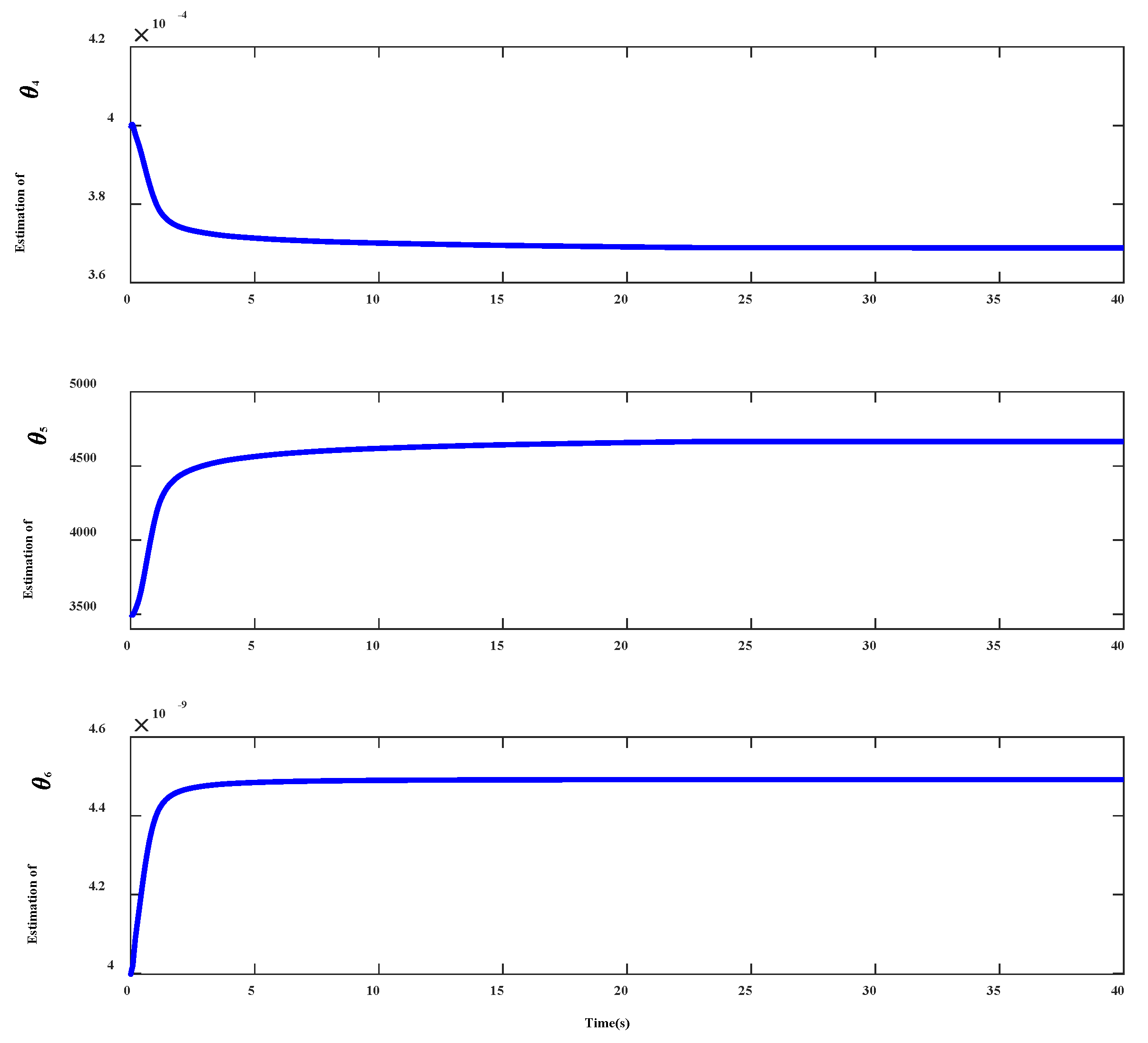
ADRAC: This controller was introduced in Section 3, and the controller parameters were provided by $k_1=200$, $k_2=50$, $k_3=30$, Γ = diag {1.1 × 10⁻⁴, 10.5, 4 × 10⁻³, 2.6 × 10⁻⁹, 1.8 × 10⁶, 3.5 × 10⁻⁷}, a₂ = 1, a₃ = 0.01, c₂ = 0.01, c₃ = 0.01, ω_o1 = 200, ω_o2 = 200, θ_max = [1, 10, 1, 1 × 10⁻², 2 × 10⁵, 1 × 10⁻⁷]^T, and θ_min = [0, 0, 0, 0, 1 × 10²,−1 × 10⁻⁷]^T. The initial parameter estimation values were set as ${\widehat{\mathit{\theta }}}_0={[0.05, 0, 0, 4\times {10}^{-4}, 3.5\times {10}^3, 4\times {10}^{-9}]}^T$.

(2)

ADRC: This is an active disturbance rejection control without parameter adaption. The difference between the ADRC and the ADRAC was that the parameter adaption matrix was set as $\mathsf{\Gamma }=0$ in the ADRC. The other control parameters were the same as the ADRAC.

(3)

AC: This is an adaptive controller without disturbance compensation. The difference between the AC and the ADRAC was that the observer parameters were set as ω_o1 = 0 and ω_o2 = 0 in AC. The other control parameters were the same as the ADRAC.

Case 1: First, a designed tracking trajectory, which had a maximum value of 45°, with maximum values of velocity and acceleration at the most at 2°/s and 2°/s², respectively, was employed to test the control performance of the developed control method. The simulation results are shown in Figure 3, Figure 4, Figure 5, Figure 6 and Figure 7. Figure 3 shows the pitch angle tracking performance and tracking error under the ADRAC controller. It can be seen that although the overall steady-state tracking error was small (i.e., the actual pitch angle could well track the desired trajectory), there was an error jump due to the non-smooth characteristics of the dead-zone break-point of the valve. This shows that the error jump caused by the non-smooth valve dead-zone could not be eliminated, although the disturbance observer-based controller could ensure the overall tracking performance. The comparison of tracking errors between the ADRAC and the other two controllers is shown in Figure 4. By comparing the tracking errors of the ADRC and the ADRAC, the transient and steady-state tracking errors were both larger than those of the ADRAC, which indicates that the adaptive law adopted in the ADRAC could learn the part of the parameter uncertainties under the same observer bandwidth, thus reducing the burden of the extended state disturbance observer and achieving better control performance. The AC controller achieved the worst tracking performance because its parameter adaptation could not achieve good convergence under the influence of uncertain nonlinearities, which also verifies the validity of the disturbance compensation technique based on the extended state disturbance observer in the ADRAC. The parameter estimations of the system under the ADRAC controller are shown in Figure 5, all of which obtained good convergence characteristics. In addition, the estimations of mismatched and matched disturbances by the extended state observer are shown in Figure 6, and the control input voltage applied to the valve with the proposed ADRAC is presented in Figure 7.

Case 2: To further test the control performance of the developed control method, a new reference tracking signal, presented in Figure 8, was adopted. Similarly, it can be seen from Figure 8 and Figure 9 that the ADRAC designed in this section still ensured the best tracking performance, which further verifies the validity of its adaptive law and extended state disturbance observer design. The parameter estimations, disturbance estimations, and control input of the ADRAC are shown in Figure 10, Figure 11, Figure 12, Figure 13 and Figure 14, respectively. Consequently, the merits of the presented control method are verified by Case 2 once again.

5. Conclusions

In this paper, an active disturbance rejection adaptive controller was developed for hydraulic lifting systems subject to parametric uncertainties, unmodeled disturbances, and a valve dead-zone. First, the dynamics, including both mechanical dynamics and hydraulic actuator dynamics with a valve dead-zone of the hydraulic lifting system, were modeled. Then, using the system model and backstepping technique, a composite parameter adaptation law and extended state disturbance observer were successfully combined, which were used to dispose of the parametric uncertainties and unmodeled disturbances, respectively. This preserved the merits of both the control methods while surmounting their practical limitations. By using the Lyapunov function, the stability of the closed-loop system was assured. A simulation example of a hydraulic lifting system was performed to verify the validity of the proposed controller.

References

1. Lu, L.; Yao, B. Energy-Saving Adaptive Robust Control of a Hydraulic Manipulator Using Five Cartridge Valves with an Accumulator. IEEE Trans. Ind. Electron. 2014, 61, 7046–7054. [Google Scholar] [CrossRef]
2. Yang, X.; Deng, W.; Yao, J. Neural Adaptive Dynamic Surface Asymptotic Tracking Control of Hydraulic Manipulators with Guaranteed Transient Performance. IEEE Trans. Neural Netw. Learn. Syst. 2022, 1–11. [Google Scholar] [CrossRef] [PubMed]
3. Xu, C.; Liu, Y.; Ding, F.; Zhuang, Z. Recognition and Grasping of Disorderly Stacked Wood Planks Using a Local Image Patch and Point Pair Feature Method. Sensors 2020, 20, 6235. [Google Scholar] [CrossRef] [PubMed]
4. Koivumaki, J.; Mattila, J. Stability-Guaranteed Force-Sensorless Contact Force/Motion Control of Heavy-Duty Hydraulic Manipulators. IEEE Trans. Robot. 2015, 31, 918–935. [Google Scholar] [CrossRef]
5. Li, L.; Lin, Z.; Jiang, Y.; Yu, C.; Yao, J. Valve deadzone/backlash compensation for lifting motion control of hydraulic manipulators. Machines 2021, 9, 57. [Google Scholar] [CrossRef]
6. Yang, X.; Deng, W.; Yao, J. Neural network based output feedback control for DC motors with asymptotic stability. Mech. Syst. Signal Process. 2022, 164, 108288. [Google Scholar] [CrossRef]
7. Sun, W.; Pan, H.; Gao, H. Filter-Based Adaptive Vibration Control for Active Vehicle Suspensions with Electrohydraulic Actuators. IEEE Trans. Veh. Technol. 2016, 65, 4619–4626. [Google Scholar] [CrossRef]
8. Yang, X.; Yao, J.; Deng, W. Output feedback adaptive super-twisting sliding mode control of hydraulic systems with disturbance compensation. ISA Trans. 2021, 109, 175–185. [Google Scholar] [CrossRef]
9. Huang, Y.; Pool, D.M.; Stroosma, O.; Chu, Q. Long-stroke hydraulic robot motion control with incremental nonlinear dynamic inversion. IEEE/ASME Trans. Mechatron. 2019, 24, 304–314. [Google Scholar] [CrossRef] [Green Version]
10. Zhang, Y.; Yan, X.; Zhang, X.; Li, J.; Cheng, F. Effects of inhomogeneity on rolling contact fatigue life in elastohydrodynamically lubricated point contacts. Ind. Lubr. Tribol. 2019, 71, 697–701. [Google Scholar] [CrossRef]
11. Kim, W.; Won, D.; Tomizuka, M. Flatness-Based Nonlinear Control for Position Tracking of Electrohydraulic Systems. IEEE/ASME Trans. Mechatron. 2014, 20, 197–206. [Google Scholar] [CrossRef]
12. Choi, Y.-S.; Choi, H.H.; Jung, J.-W. Feedback Linearization Direct Torque Control with Reduced Torque and Flux Ripples for IPMSM Drives. IEEE Trans. Power Electron. 2016, 31, 3728–3737. [Google Scholar] [CrossRef]
13. Yao, B.; Al-Majed, M.; Tomizuka, M. High-performance robust motion control of machine tools: An adaptive robust control approach and comparative experiments. IEEE/ASME Trans. Mechatron. 1997, 2, 63–76. [Google Scholar]
14. Yao, B.; Bu, F.; Reedy, J.; Chiu, G.T.C. Adaptive robust motion control of single-rod hydraulic actuators: Theory and experiments. IEEE/ASME Trans. Mechatron. 2000, 5, 79–91. [Google Scholar]
15. Lyu, L.; Chen, Z.; Yao, B. Advanced valves and pump coordinated hydraulic control design to simultaneously achieve high accuracy and high efficiency. IEEE Trans. Control. Syst. Technol. 2021, 29, 236–248. [Google Scholar] [CrossRef]
16. Yang, X.; Ge, Y.; Deng, W.; Yao, J. Adaptive dynamic surface tracking control for uncertain full-state constrained nonlinear systems with disturbance compensation. J. Frankl. Inst. 2022, 359, 2424–2444. [Google Scholar] [CrossRef]
17. Deng, W.; Yao, J.; Ma, D. Time-varying input delay compensation for nonlinear systems with additive disturbance: An output feedback approach. Int. J. Robust Nonlinear Control 2018, 28, 31–52. [Google Scholar] [CrossRef]
18. Deng, W.; Yao, J. Asymptotic tracking control of mechanical servosystems with mismatched uncertainties. IEEE/ASME Trans. Mechatron. 2021, 26, 2204–2214. [Google Scholar] [CrossRef]
19. Deng, W.; Yao, J.; Wang, Y.; Yang, X.; Chen, J. Output feedback backstepping control of hydraulic actuators with valve dynamics compensation. Mech. Syst. Signal Process. 2021, 158, 107769. [Google Scholar] [CrossRef]
20. Ge, Y.; Yang, X.; Deng, W.; Yao, J. Rise-based composite adaptive control of electro-hydrostatic actuator with asymptotic stability. Machines 2021, 9, 181. [Google Scholar] [CrossRef]
21. Xiong, T.; Gu, Z.; Yi, J.; Pu, Z. Fixed-Time Adaptive Observer-Based Time-Varying Formation Control for Multi-Agent Systems with Directed Topologies. Neurocomputing 2021, 463, 483–494. [Google Scholar] [CrossRef]
22. Won, D.; Kim, W.; Tomizuka, M. High-gain-observer-based integral sliding mode control for position tracking of electrohydraulic servo systems. IEEE/ASME Trans. Mechatron. 2017, 22, 2695–2704. [Google Scholar] [CrossRef]
23. Rath, J.J.; Defoort, M.; Karimi, H.R.; Veluvolu, K.C. Output Feedback Active Suspension Control with Higher Order Terminal Sliding Mode. IEEE Trans. Ind. Electron. 2017, 64, 1392–1403. [Google Scholar] [CrossRef]
24. Yao, J.; Jiao, Z.; Ma, D. Extended-state-observer-based output feedback nonlinear robust control of hydraulic systems with backstepping. IEEE Trans. Ind. Electron. 2014, 61, 6285–6293. [Google Scholar] [CrossRef]
25. Wang, S.; Tao, L.; Chen, Q.; Na, J.; Ren, X. USDE-Based Sliding Mode Control for Servo Mechanisms with Unknown System Dynamics. IEEE/ASME Trans. Mechatron. 2020, 25, 1056–1066. [Google Scholar] [CrossRef]
26. Ba, D.X.; Dinh, T.Q.; Bae, J.; Ahn, K.K. An Effective Disturbance-Observer-Based Nonlinear Controller for a Pump-Controlled Hydraulic System. IEEE/ASME Trans. Mechatron. 2020, 25, 32–43. [Google Scholar] [CrossRef]
27. Deng, W.; Yao, J. Extended-State-Observer-Based Adaptive Control of Electrohydraulic Servomechanisms without Velocity Measurement. IEEE/ASME Trans. Mechatron. 2020, 25, 1151–1161. [Google Scholar] [CrossRef]
28. Merritt, H. Hydraulic Control Systems; John Wiley & Sons: Hoboken, NJ, USA, 1967. [Google Scholar]
29. Deng, W.; Yao, J.; Ma, D. Robust adaptive precision motion control of hydraulic actuators with valve dead-zone compensation. ISA Trans. 2017, 70, 269–278. [Google Scholar] [CrossRef]
30. Yao, J.; Jiao, Z.; Ma, D.; Yan, L. High-accuracy tracking control of hydraulic rotary actuators with modeling uncertainties. IEEE/ASME Trans. Mechatron. 2014, 19, 633–641. [Google Scholar] [CrossRef]
31. Krstic, M.; Kanellakopoulos, I.; Kokotovic, P. Nonlinear and Adaptive Control Design; Wiley: New York, NY, USA, 1995. [Google Scholar]
Figure 1. A sketch of the lifting system.
Electronics 11 01788 g001
Figure 2. The valve dead-zone characteristics.
Electronics 11 01788 g002
Figure 3. The tracking performance of the ADRAC.
Electronics 11 01788 g003
Figure 4. The tracking errors of the three controllers.
Electronics 11 01788 g004
Figure 5. The parameter estimations of θ1~θ3 with the ADRAC.
Electronics 11 01788 g005
Figure 6. The parameter estimations of θ4~θ6 with the ADRAC.
Electronics 11 01788 g006
Figure 7. The disturbance estimations of the ADRAC.
Electronics 11 01788 g007
Figure 8. The control input of the ADRAC.
Electronics 11 01788 g008
Figure 9. The tracking performance of the ADRAC.
Electronics 11 01788 g009
Figure 10. The tracking errors of the three controllers.
Electronics 11 01788 g010
Figure 11. The parameter estimations of θ1~θ3 with the ADRAC.
Electronics 11 01788 g011
Figure 12. The parameter estimations of θ4~θ6 with the ADRAC.
Electronics 11 01788 g012
Figure 13. The disturbance estimations of the ADRAC.
Electronics 11 01788 g013
Figure 14. The control input of the ADRAC.
Electronics 11 01788 g014