A Bayesian Optimization Approach for Multi-Function Estimation for Environmental Monitoring Using an Autonomous Surface Vehicle: Ypacarai Lake Case Study

Abstract

Bayesian optimization is a sequential method that can optimize a single and costly objective function based on a surrogate model. In this work, we propose a Bayesian optimization system dedicated to monitoring and estimating multiple water quality parameters simultaneously using a single autonomous surface vehicle. The proposed work combines different strategies and methods for this monitoring task, evaluating two approaches for acquisition function fusion: the coupled and the decoupled techniques. We also consider dynamic parametrization of the maximum measurement distance traveled by the ASV so that the monitoring system balances the total number of measurements and the total distance, which is related to the energy required. To evaluate the proposed approach, the Ypacarai Lake (Paraguay) serves as the test scenario, where multiple maps of water quality parameters, such as pH and dissolved oxygen, need to be obtained efficiently. The proposed system is compared with the predictive entropy search for multi-objective optimization with constraints (PESMOC) algorithm and the genetic algorithm (GA) path planning for the Ypacarai Lake scenario. The obtained results show that the proposed approach is 10.82% better than other optimization methods in terms of R2 score with noiseless measurements and up to 17.23% better when the data are noisy. Additionally, the proposed approach achieves a good average computational time for the whole mission when compared with other methods, 3% better than the GA technique and 46.5% better than the PESMOC approach.

1. Introduction

Monitoring water resources is a very useful practice for their maintenance. The results obtained by supervision campaigns can be used as a key tool for efficient decision-making regarding the protection of water bodies, such as reservoirs, lakes, and lagoons, against climate change damage and other threats. The limnology or study of inland aquatic ecosystems is fundamentally based on observing the water environment chemical, physical, and biological characteristics. A water quality level can be determined by taking into account these features through several chemical and physical indicators or variables, such as pH, temperature, total suspended solids, and dissolved oxygen, among others. These parameters are part of the biological characteristics that a water body can acquire. Therefore, monitoring the behavior of quality parameters of water masses represents a valuable mission due to its involvement in the maintenance of healthy aquatic environments. Examples of dramatic scenarios, from the water quality indicators point of view, include those in which an excessive amount of nutrients exist in their waters so that green-blue algae (cyanobacteria) blooms proliferate. This situation is harmful for the ecosystem because these algae are known to be toxic not only to fauna and aquatic plants but also to humans. Some examples of lakes [1] having this issue include Ypacarai Lake (San Bernardino, Paraguay) and Lake Titicaca (El Collao, Perú). Consequently, monitoring the water quality state of these lakes is crucial for eradicating the algae blooms and restoring the freshness and quality of their waters [2].

Generally, monitoring missions consist of both manual measurement campaigns and fixed stations located at the water resources. However, in some scenarios, the manual procedure exposes the human operator to the danger of toxic waters while maneuvering the measurement equipment. Regarding the utilization of fixed stations, it fails to provide a global state of the water quality, which is more aggravated for large water resources, leading to wrong estimations. Thus, these mechanisms present several disadvantages with respect to recent distributed approaches, such as using autonomous surface vehicles (ASVs) equipped with water quality sensors (see Figure 1). For instance, the use of ASVs significantly decreases the mission costs by allowing automated sampling [3]. The current literature shows a vast amount of environmental monitoring systems using ASVs, ranging from intelligent patrolling [4] to informative path planning (IPP) approaches [5]. These systems are very useful and have significant advantages when compared to manual or fixed monitoring tools. However, the majority of the proposed systems are focused on pure exploration methods, without aiming to obtain a surrogate function or regression model that represents and predicts the behavior of water quality parameters in unexplored locations. Another main limitation of the existing systems corresponds to the non-generalized data acquisition paradigm because they are focused on a single parameter acquisition; i.e., they only focus on obtaining data taking into account only one water quality parameter. However, most water quality sensor systems are capable of performing multiple measurements at the same time (multi-probe systems). In addition, battery autonomy is another main constraint in current monitoring systems based on ASVs. Consequently, the mobility of vehicles should be determined carefully to accomplish efficient monitoring campaigns.

This work is focused on alleviating the aforementioned limitations of current monitoring systems based on ASVs. First, we propose using Gaussian process (GP) to estimate models of water quality parameters with small datasets of real measurements. GP-based regressors are suitable for modeling in those scenarios. Thus, they remove the necessity of monitoring every location of the lake, saving time, money, and human resources. Second, we consider a multi-function estimation framework for modeling several water quality parameters simultaneously. Therefore, we propose a generalized monitoring system with multiple data acquisition functions. Third, we take into account the mobility restrictions of ASVs with respect to available battery energy by limiting the distance traveled by the ASV among measurements. The proposed system is based on a previous work and it enhances the single Bayesian optimization (BO) approach, allowing it to intelligently select measurement locations so that all three requirements are satisfied. Thus, we propose a multi-function estimation using Bayesian Optimization (MEBO) approach for environmental monitoring through a single ASV.

The classical BO approach consists of sequentially selecting new measurement locations according to an acquisition function (AF). The AF determines the benefit/value of sampling in an unknown location according to maximizing a single target function. However, whenever multiple target functions are considered, different AFs are obtained simultaneously for each one of them, resulting in a multi-function estimation scenario. Then, the question is how to combine or fusion the different AFs to determine the next location to sample.

We extend the proposed AFs in [5] by adding AF Fusion (AFF) methods for providing measurement locations. These fusion methods balance the desirability of taking measurements on certain locations in order to decrease uncertainties on several water quality maps simultaneously. The proposed MEBO considers and evaluates two different AFFs, the coupled and decoupled techniques. The former combines the different AFs for providing an overall optimal measurement location, while the latter provides the best location according to the simple evaluation of different AFs. Consequently, the MEBO for environmental monitoring approach consists of (i) defining surrogate models for all the unknown water quality parameters; (ii) fitting these surrogate models with measured data; (iii) acquiring new measurement locations according to a fusion of AFs; and, finally, (iv) reaching the destination point, performing new measurements. and adding such data to the data set.

The main contributions of this work can be summarized as follows:

• A generalized multi-parameter measuring system for environmental monitoring based on Bayesian optimization with acquisition function fusions.
• An experimental study of data sampling distance between measurements using kernel hyper-parameters information.
• A validation and comparison with other approaches in a real-case scenario such as the monitoring of Ypacarai Lake in Paraguay.

The present work is divided into the next sections. Section 2 includes the related works found in the literature. Next, in Section 3, the statement of the problem is described. Afterwards, Section 4 presents the proposed MEBO approach. The surrogate model’s performance and computational evaluation of the proposed method and the related methods, as well as the discussion of the results, are available in Section 5. Finally, the conclusion and future works are presented in Section 6.

2. Related Works

This section is divided into two parts: first, several works that use autonomous vehicles, both aerial and aquatic, for environmental monitoring tasks are presented; second, some works related to multi-Bayesian optimization are reviewed.

2.1. Environmental Monitoring with Autonomous Vehicles

The application of monitoring based on autonomous vehicles is an active research field [6,7]. Both aerial and aquatic (surface and underwater) vehicles have been proposed to measure environmental variables. Such is the case of the work in [8] that proposes a Q-learning fuzzy logic for flying ad hoc networks. Another work [9] develops aerial vehicles’ path-planning strategies for autonomous search and localization of targets in a risky environment while optimizing both search and survival via the selection of a balance Pareto-point front and using customized reward functions. A recent study [10] designs a multi-objective optimization for drone delivery that manages to minimize the delivery cost using the $ϵ$-constraint method and the percentage of unsuccessful delivered packages while maximizing the on-time delivery reward. The MO strategy is also proposed in [11], where a coverage problem is addressed using multiple aerial vehicles for efficient communication networks. Related to monitoring, in [12], the authors describe a path generation algorithm that minimizes time of rescue action using a genetic algorithm (GA) technique. The work takes into account several dynamic and time constraints in order to provide efficient routes for reaching a target destination. Another approach [13] considers multiple aerial vehicles for agricultural monitoring using a distributed swarm control technique.

Works using ASVs for environmental monitoring, specifically for lakes, can be found in the literature [3,4,5,14,15,16]. However, they are generally focused on one objective such as minimizing the uncertainty of one water quality parameter. In [4], a deep reinforcement learning (DRL) approach was designed so that a single ASV patrolled the Lake. In [14], the authors generalize the DRL to a multi-agent ASV using an enhanced approach. The work also compares different deep reinforcement learning approaches, such as double DRL and dueling DRL, for multi-ASV missions. The work in [3] aims at obtaining a sequence of visiting beacons at the Ypacarai Lake, using the travelling salesman problem (TSP) definition and the use of evolutionary approaches (GA) to define the best sequence. The mentioned work was further improved and compared with Hamiltonian circuits in [15]; the evolutionary-based approach manages to obtain the best visiting order so that the maximum possible area coverage is performed. Additional improvements were proposed in [16], where two objectives (exploration and exploitation) are accomplished but not simultaneously. The Ypacarai Lake environmental monitoring problem was also addressed [5] with a BO approach using a single ASV with a single water quality sensor. In the mentioned work, the authors describe adaptations of AFs so that mobility constraints of ASV are taken into account.

Table 1. Brief summary of related works. Specifying whether the work is Multi-Objective (MO) or not.

Ref.	Specific Objective	Is MO?	Main Algorithm	Vehicle	Year
[9]	Search for targets in risky environments	Yes	Pareto-front point selection	Aerial	2018
[13]	Agricultural field coverage	No	Distributed swarm control	Aerial	2018
[10]	Package delivery pptimization	Yes	$ϵ$-constraint method	Aerial	2019
[3]	Pure exploration	No	TSP and genetic algorithm	ASV	2019
[16]	Exploration and intensification	No	Hamiltonian and Eulerian circuits	ASV	2019
[8]	Routing algorithms for Comms.	Yes	Q-learning fuzzy logic	Aerial	2020
[12]	Time-efficient path planning	No	Genetic algorithm	-	2020
[4]	Monitoring through patrolling	No	Double deep Q-learning	ASV	2020
[11]	Wireless network coverage	Yes	Simulated annealing	Aerial	2020
[5]	Monitoring and model obtaining	No	Bayesian optimization	ASV	2021
[14]	Multi-agent monitoring	No	Double deep Q-learning	ASV	2021

shows a summary of related works. The mentioned works can be related to our work in terms of MO, monitoring missions, or applications. The works are ordered by year of publication.

2.2. Multi-Objective Optimization

Multi-Objective Bayesian Optimization has been applied to many optimization works [17,18] in several research fields. Although the MEBO has not been used in monitoring systems with autonomous vehicles, the sequential BO proposed in the existing works is useful and can be adapted to accomplish monitoring tasks. For example, in [17], a predictive entropy search for multi-objective BO with constraints (PESMOC) is proposed using a four-step process. This method takes into account the Pareto-front generated by a set of predicted mean distributions. The general PES AF is used for each objective function. In addition, the authors propose both coupled and decoupled methods to fuse the different AFs. The first fusion technique consists of adding the different AFs in order to obtain a global AF. However, the second method, which consists of selecting the maximum of the different AFs, has been proven to generate better results. In this work, the same terms for the fusion of different AFs are adopted, and the appropriate definition and expressions can be found in Section 4. On the other hand, in [18], the authors used a two-stage BO for global optimization based on the evaluation of multiple AFs using the same surrogate model and a selection criterion, obtaining a reward-based AF selection system. However, in the mentioned work [18], the system is capable of evaluating the objective function without accounting for distance between measurements locations, so that, ultimately, multiple AFs (one for each objective) were used only for increasing the total number of measurements.

Furthermore, multi-objective optimization systems using fixed sensor stations have been recently proposed for different environmental missions, such as ventilation system monitoring [19] or even water quality monitoring [20]. Both mentioned works pursue the objective of optimally positioning sensors in fixed locations. While the former [19] uses a GA for obtaining the optimal locations according to several functions, the latter [20] utilizes transinformation entropy, which measures mutual information, to be minimized by an enhanced GA for multi-objective optimization. These methods consider the multiple objectives and solves the problem by taking into account each objective independently, like the decoupled method in [17]. For coverage problems taking into account multiple vehicles, in [21], the authors propose a coupled weighted multi-function for deciding positions of UAVs for optimal coverage deployments. These works base the selection of locations on GA.

Finally, the proposed method differentiates from the related works as it is the first, to the best known of the authors, that addresses the multi-objective data acquisition for environmental monitoring using ASVs. The MEBO system is capable of minimizing the uncertainty, which minimizes the surrogate error of multiple water quality models simultaneously. Furthermore, we manage to implement MO optimization approaches for environmental monitoring, whereas recent MO algorithms are not tested in this scenario. When comparing to the fixed station works, the proposed MEBO method can efficiently select measurement locations when the functions are unknown, whereas the fixed monitoring station methods are based on monitoring environments with a priori information. With respect to other ASV-based environmental monitoring systems, the MEBO system is actively learning, exploring the environment taking into account multiple information due to the fact that it is based on Bayesian optimization for multiple functions. In addition, contrary to the constant distance between measurement locations approach proposed in [5], the MEBO approach in this work aims at generalizing this distance based on a relationship with the length-scale hyper-parameter of the surrogate model, which at the same time, is related to the real behavior of the objective functions. Therefore, the proposed approach actively updates another high-level hyper-parameter for monitoring.

3. Statement of the Problem

3.1. Objective Functions

The target consists of minimizing the error of a set of functions simultaneously, using the next expression:

$$\begin{array}{c}\hfill \mathrm{minimize}\{{\displaystyle \sum _{i=1}^{i=n}}{\mathcal{F}}_i\left(\mathbf{x}\right)\}\\ \hfill \mathbf{s}\mathbf{.}\mathbf{t}\mathbf{.}\mathbf{x}\in \mathcal{X}\end{array}$$

(1)

In the expression shown above, ${\mathcal{F}}_i\left(\mathbf{x}\right)$ is one of the n functions to be minimized, i.e., ${\mathcal{F}}_1\left(\mathbf{x}\right),{\mathcal{F}}_2\left(\mathbf{x}\right),\dots ,{\mathcal{F}}_n\left(\mathbf{x}\right)$. Generally, no solution exists that simultaneously minimizes all functions since the objectives are counterbalanced; i.e., the value that minimizes ${\mathcal{F}}_i\left(\mathbf{x}\right)$ is not equal to the value for minimizing any other function ${\mathcal{F}}_i\left(\mathbf{x}\right)$. $\mathcal{X}$ is a m-sized set, which corresponds to the feasible search space.

In the context of this work, each function ${\mathcal{F}}_i\left(\mathbf{x}\right)$ corresponds to the error of a surrogate model of a water quality parameter i with respect to the real behavior of the same parameter in the Ypacarai Lake. In that way, since errors will be minimized on all surrogate models, good surrogate models of water quality parameters will be obtained simultaneously. This work considers each function ${\mathcal{F}}_i\left(\mathbf{x}\right)$ as the mean squared error (MSE) regression loss, which evaluates the average of squared difference between a real or objective function $f_i\left(\mathbf{x}\right)$ and the surrogate or approximated regression $\widehat{f_i}\left(\mathbf{x}\right)$. The MSE for a given parameter i is calculated over $\mathcal{X}$ (size m) using the following expression:

$${\mathrm{MSE}}_i(f_i\left(\mathbf{x}\right),{\widehat{f}}_i\left(\mathbf{x}\right))=\frac{1}{m}\sum {(f_i\left(\mathbf{x}\right)-{\widehat{f}}_i\left(\mathbf{x}\right))}^2$$

(2)

Minimizing the expression above consists of obtaining appropriate surrogate functions ${\widehat{f}}_i\left(\mathbf{x}\right)$, since m and $f_i\left(\mathbf{x}\right)$ are constant. Therefore, the multi-function estimation mission will be accomplished whenever surrogate models are as similar as possible to the true functions:

$${\widehat{f}}_i\left(\mathbf{x}\right)\approx f_i\left(\mathbf{x}\right)+{\mathcal{E}}^2$$

(3)

The function ${\mathcal{E}}^2$ corresponds to the inherent noise associated to surrogate modeling procedures, such as objective function evaluations and error modeling. Specifically, in water quality parameter modeling, errors include sensor and location measurement inaccuracies [5].

Furthermore, in the present work, $f_i\left(\mathbf{x}\right)$ corresponds to the real water quality behavior of parameter i, where $\mathbf{x}$ corresponds to a $(x,y)$ location of the Ypacarai Lake ($\mathcal{X}\subset {\mathbb{R}}^2$). These functions $f_i\left(\mathbf{x}\right)$ are available for sensing, and measurements will be taken by a single ASV equipped with a set water quality sensors, which provides a read of the value of parameter i at location $p_k\in \mathbf{x}$ (Equation (4)). The subscript k corresponds to the measurement number of o total measurements, where $p_k$ is usually used to denote the location of the last performed measurement.

$$s_{(k,i)}=f_i\left(p_k\right)+{ϵ}^2$$

(4)

Each set of measurements, which contains information of the location $p_k$ and the values of parameters at that location $s_{(k,i)}$, is stored in data set D. As mentioned, the measurements can be noisy and their values may differ from real data. Therefore, in Equation (4), ${ϵ}^2$ represents the supposed iid noise drawn from function ${\mathcal{E}}^2$. The data set D provides sufficient information to the MEBO system so that, for every parameter, a function ${\widehat{f}}_i$ can be approximated.

3.2. Assumptions

Next, some assumptions and considerations are established so that the full scope of our work is defined according to the main objective presented at the start of this section.

• Environment: The environment consists of a defined region modelled as a matrix $\mathcal{M}$. The matrix $\mathcal{M}$ corresponds to the square grid representation of real-life locations (latitude, longitude). Therefore, the real environment is discrete, meaning that an ASV can be located in a position related to an element of the map. Every element ${\mathcal{M}}_{i,j}$ is a square of side d, and this can be navigable or occupied by an impassable object (such as terrain or obstacles). The full set of navigable elements or squares corresponds to $\mathcal{X}$:

  $$\mathcal{X}\subseteq \mathcal{M}\subseteq {\mathbb{R}}^2$$

  (5)

  If element ${\mathcal{M}}_{i,j}$ is navigable, it is considered a part of the water body and has measurable properties (set $\mathcal{X}$). Therefore, all navigable locations in the set $\mathcal{X}$ are available for reading, meaning that there exists a water quality map ${\mathcal{S}}_i$ for each studied water quality parameter. The water quality values of each map ${\mathcal{S}}_i$ on location $\mathbf{x}\in \mathcal{X}$ are considered time invariant, i.e., they remain constant through the simulations. All ${\mathcal{S}}_i$ maps of water quality parameters follow the main characteristic of the central distribution theorem, implying that the expected mean is zero and the standard deviation is one. However, the values are not necessarily normally distributed around the center of the Lake. Another important assumption implies that the behaviors of water quality parameters are smooth and continuous, mainly due to fluid dynamics and surface wave propagation properties [5]. Figure 2 shows an example of Ypacarai Lake modelled as matrix $\mathcal{M}$, as determined with a procedure found in [22]. This model gives $\mathcal{X}$ the characteristic of being non-convex; i.e., not all segments made with two different locations $\mathbf{x}$ and ${\mathbf{x}}^{\prime }$ can be divided into segments that contain only elements of $\mathcal{X}$.
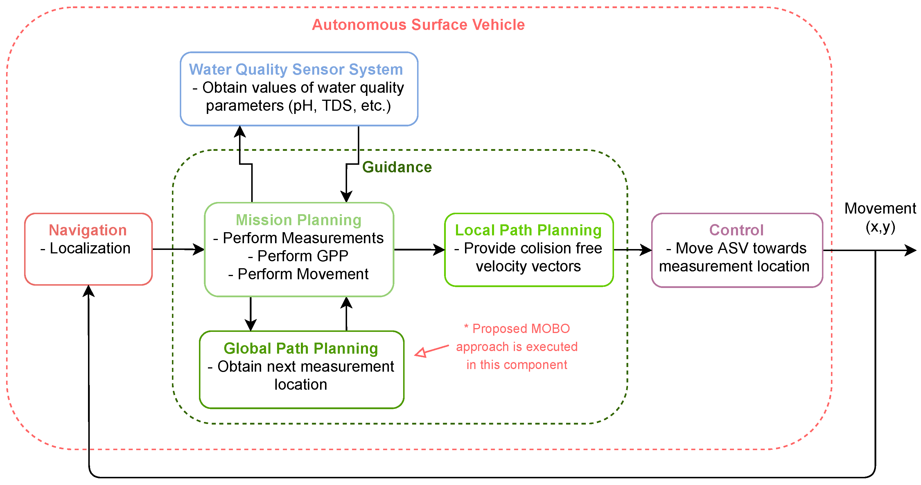
• Navigation, Guidance, and Control (NGC) System: The ASV has subsystems that are designed for specific purposes of navigation, guidance, and control. Figure 3 depicts the general system design. The ASV contains the NGC system so that it can autonomously position, decide missions, and move for accomplishing the objective. The navigation subsystem is in charge of locating the vehicle; however, the positioning system is not perfect and can provide the position of the ASV within a circle of radius r. This positioning error leads to guidance inaccuracies. The guidance subsystem is in charge of planning paths. Once a goal is defined using a global path planner (GPP) component, which implements the MEBO approach, this subsystem defines a collision-free path from the current position of the ASV to the goal location. If no obstacles are in the segment, a direct route is planned; otherwise, the guidance system plans a path using RRT*, as it can provide quick, good paths as shown in [23]. Finally, the control subsystem is in charge of reaching the calculated goal, but as the navigation subsystem has an error of $\pm 2r$, the measurement position $p_k\in \mathbf{x}$ may be shifted by $\pm 3r$. This error also accounts for water and air currents, stopping mechanisms, etc.
• Water Quality Sensor System: The vehicle is supposedly equipped with n water quality sensors named $s_1,s_2,\dots ,s_n$. It can be observed in Figure 3 that the ASV communicates the water quality sensor system to the mission planning component through the guidance system. The guidance system commands the performing of measurements, and the sensor system provides the values of water quality parameters. These sensors can measure different variables simultaneously, but the ASV needs to stop to take measurements. This constraint prevents continuous monitoring; i.e., the vehicle cannot be constantly obtaining new information. As shown in Equation (4), the sensors do not perform perfect measurements; therefore, noise is present in every read. For real purposes, the values returned by the sensors are not normally distributed ($\mu \left(\mathbf{x}\right)=0$, $\sigma \left(\mathbf{x}\right)=1$); therefore, additional data pre-processing is needed to ensure that the values that are fed to the MEBO system will have the mentioned characteristics. Preprocessing data is a common procedure in machine learning, and it is used in this work to facilitate the fitting of Gaussian process models with means of zero.
• ASV constraints: The ASV has a smaller size than the size d of a square of matrix $\mathcal{M}$ so that a movement in every direction is always possible. For performance evaluation purposes, the battery autonomy is taken into account. In order to include battery usage, one approach is to consider its level as a function constraint, but since the battery level is independent of the position p of the vehicle (i.e., the input in the proposed MEBO approach), this constraint cannot be approximated to a function of $(x,y)$. Therefore, methods to include the battery level directly in the BO method as a constraint, such as the work in [17], cannot be used. Consequently, in this work, as in a related work [5], we consider that missions finalize whenever the ASV travels a total distance of 15,000 m, which corresponds to approximately $2.1$ h of usage.

With the assumptions defined, we remark that, as for the problem, water quality measurement locations must be strategically selected. The designed MEBO should balance travelling distance and taking measurements so that enough data are collected from the environment in order to provide good surrogate water quality models. The scopes of this work consider that the average MSE is to be minimized sequentially, meaning that on every step k, the errors of multiple surrogate functions are to be simultaneously minimized after performing one measurement in position $p_k$. Nonetheless, since in a real execution access to the function $f_i\left(x\right)$ is not possible, the calculation of the MSE is also not possible. Therefore, we base the proposed monitoring system on obtaining probabilistic surrogate models, which have bounded uncertainty maps, so that we pivot from minimizing error to minimizing uncertainty maps and assume that uncertainties of surrogate models are correlated to the error of these models.

4. Proposed Approach

The proposed system is based on the general single BO approach for monitoring [5], where a sequential strategy evaluates the current state of a water quality parameter and then proceeds to select new informative measurement locations that enhance the model of the selected parameter. In this work, we generalize to multiple parameters with the use of multiple information gathering and evaluating. Figure 4 shows the proposed procedure, where the classical BO approach is enhanced to consider multiple surrogate models for selecting the new measurement locations. The proposed MEBO is adapted in order to favor exploration during the whole mission. First, we define the components of the BO approach and then we expand the method in order to include the multi-function estimation goal. In that sense, until Section 4.4, the problem is treated as a single-objective BO, i.e., $i=1$. Therefore, the expressions are defined for the monitoring of a single water quality parameter. Afterwards, we retake the MEBO approach, i.e., $i=[1,2,\dots ,n]$.

4.1. Bayesian Optimization

BO is the proposed sequential strategy for environmental monitoring [5]. It is generally used for optimizing an unknown objective function that is expensive to evaluate [24], i.e., finding the minimum/maximum of the objective. In the case of environmental monitoring, the direct application of BO will not provide good surrogate models, as the functions will be directed to optimize the ground truth model. Nevertheless, with the modification of parameters and the adjustment of functions, the BO approach can be used to reduce the uncertainty of surrogate models so that the MEBO approach is capable of providing good surrogate models of water quality parameters.

In a general sense, BO provides the location where the next measurement should be performed $p\ast =p_{k+1}$. This location is obtained using the next expression:

$$\begin{array}{c}\hfill p\ast ={\mathrm{argmax}}_{\mathbf{x}}\left\{g\left(\mathbf{x}\right)\right\}\\ \hfill \mathbf{s}\mathbf{.}\mathbf{t}\mathbf{.}g\left(\mathbf{x}\right)=\alpha (\widehat{f}\left(\mathbf{x}\right))\end{array}$$

(6)

where the function $g\left(\mathbf{x}\right)$ needs to be maximized, according to [25]. The function argument of Equation (6) is decomposed into an acquisition function ($\alpha$) and a surrogate model $\widehat{f}\left(\mathbf{x}\right)$. As the AF depends directly on the surrogate model, first, this model should be appropriately defined. Many authors [17,25,26,27] use Gaussian processes as probabilistic surrogate models since they present important advantages for modeling unknown functions.

4.2. Gaussian Processes

Using a model-based regression whenever the unknown function has a predictable behavior presents several advantages, if the surrogate model can fit the data. GP Regressions are model-based processes [24], where prior and posterior models can be generated using two sets of information: (i) the relationships between the unknown data and (ii) the sampled data. The latter set corresponds to data D (recall Equation (4)), while the relationship information corresponds to the covariance function, which measures the similarity between the inputs. GPs are based on multivariate normal distributions; i.e., for each position $\mathbf{x}$, a mean $\mu \left(\mathbf{x}\right)$ and a variance ${\sigma }^2\left(\mathbf{x}\right)$ can be obtained. For that reason, one of the main advantages of using GPs is that they do not only provide the expected behavior of the objective function but also an uncertainty measure of the output, namely, the standard deviation.

For appropriately specifying GPs, only a tuple of the mean and the covariance function is need:

$$\begin{array}{cc}\hfill \mu \left(\mathbf{x}\right)& =\mathbb{E}\left[f\right(\mathbf{x}\left)\right]\hfill \\ \hfill k(\mathbf{x},{\mathbf{x}}^{\prime })& =\mathbb{E}\left[(f\left(\mathbf{x}\right)-\mu \left(\mathbf{x}\right))(f\left({\mathbf{x}}^{\prime }\right)-\mu \left({\mathbf{x}}^{\prime }\right))\right]\hfill \end{array}$$

(7)

The mean corresponds to the expected output of the objective function, while the covariance between one specific position $\mathbf{x}$ and another ${\mathbf{x}}^{\prime }$ is equal to the expected product of differences. If the covariance function can fit the provided data D, the GP mean can be taken as the surrogate function output as:

$$\widehat{f}\left(\mathbf{x}\right)\sim \mathcal{GP}(\mu \left(\mathbf{x}\right),k(\mathbf{x},{\mathbf{x}}^{\prime }))=\mathcal{N}(\mu \left(\mathbf{x}\right),\sigma \left(\mathbf{x}\right))$$

(8)

Note that the predicted function $\widehat{f}\left(\mathbf{x}\right)$ using GPs consists of a normal distribution with a mean $\mu \left(\mathbf{x}\right)$ and a variance ${\sigma }^2\left(\mathbf{x}\right)$. Nonetheless, in this section, we refer to $\widehat{f}\left(\mathbf{x}\right)$ simply as the mean output $\mu \left(\mathbf{x}\right)$ of the GP, except when indicated otherwise. Before solving Equation (8), it is preferable to define the covariance function, as well as the kernel matrix.

Covariance functions imposes the geometry of the model [25] due to the fact that they define the relationships between input features. In this work, we define the features as the 2D positions where the model needs to be obtained, that is, all positions of set $\mathcal{X}$. Therefore, the covariance function, sometimes called kernel, should be able to describe the generalized behavior function of a real water quality parameter. As assumed in Section 3, it is expected that the water quality parameters are time invariant, smooth, and continuous. Therefore, the kernels of the GPs in this work should provide similar properties to the approximated output.

The evaluations of the covariance function for each pair of inputs ($\mathbf{x}$ and ${\mathbf{x}}^{\prime }$) can be grouped in a square matrix $\mathbf{K}$, where each element ${\mathbf{K}}_{i,j}=k({\mathbf{x}}_i,{\mathbf{x}}_j)$. Therefore, this matrix, named kernel matrix, will be symmetric and, since its construction is based on the inputs, it will also follow the same properties as the Gram matrix, which is semi-positive definite. The complete covariance matrix for all possible locations $\mathbf{x}$ is defined as

$$\begin{array}{c}\mathbf{K}=\left[\begin{array}{cc}K& K_{*}\\ K_{*}^T& K_{**}\end{array}\right]=\left[\begin{array}{cc}k(\mathbf{x},\mathbf{x})& k(\mathbf{x},{\mathbf{x}}_{*})\\ k({\mathbf{x}}_{*},\mathbf{x})& k({\mathbf{x}}_{*},{\mathbf{x}}_{*})\end{array}\right]\end{array}$$

(9)

where the unknown input data ${\mathbf{x}}_{*}$ correspond to a subset of $\mathcal{X}$ (Equation (5)) that needs to be approximated, since no measurements were performed in those positions. The remaining subset ($\mathbf{x}$ of the preceding expression) corresponds to every measurement location $p_k\mathbf{s}\mathbf{.}\mathbf{t}\mathbf{.}k=[1,2,\dots ,o]$. Therefore, for obtaining the kernel matrix, $\mathcal{X}$ is effectively divided into two sets of known and unknown input data: $\{\mathbf{x},{\mathbf{x}}_{*}\}$. Then, K is a square matrix made with the covariance values between the known input data; $K_{*}$ is a rectangular matrix made with the known input data as rows and the unknown input data as columns; and, lastly, $K_{**}$ is, again, a square matrix but with rows and columns defined by the unknown input data.

Finally, to solve the GP for unknown input data ${\mathbf{x}}_{*}$, Equation (10) is used [24], where a new term ${ϵ}^{2}I$ is added in order to provide the GP with noise, whenever the measured values $\widehat{f}\left(\mathbf{x}\right)$ are known to be noisy (Equation (3)).

$$\begin{array}{c}\hfill {\mu }_{\widehat{f}\left({\mathbf{x}}_{*}\right)\mid D}=K_{*}^T{(K+{ϵ}^{2}I)}^{-1}\widehat{f}\left(\mathbf{x}\right)\\ \hfill {\sigma }_{\widehat{f}\left({\mathbf{x}}_{*}\right)\mid D}=K_{**}-K_{*}^T{(K+{ϵ}^{2}I)}^{-1}{K}_{*}\end{array}$$

(10)

The expression shown above is sufficient to solve the problem for the unknown inputs or non-measured locations of the Ypacarai Lake. It is important to highlight that the inference will not be appropriate if the kernel does not behave as the real function. The definition of the kernel should be always aimed to fit the unknown objective function. Therefore, for the monitoring task, the selected kernel should follow the same behavior as water quality parameters of still waters (surface currents $<2\frac{\mathrm{m}}{\mathrm{s}}$ [5]). Most authors [25,26] use the radial basis function (RBF) kernel since it can easily fit stationary data and due to the fact that it is infinitely differentiable (continuous).

RBF is a real-valued covariance function whose values depend solely on the distances between the inputs $\mathbf{x}$ and ${\mathbf{x}}^{\prime }$, which defines it as a stationary kernel, i.e., the kernel does not depend on the position of the inputs but on the relative difference of them. The RBF also depends on a hyper-parameter ℓ, which modifies the maximum distance of influence between the inputs. The RBF has the form of

$$k{(\mathbf{x},{\mathbf{x}}^{\prime })}_{\mathrm{RBF}}=\exp (-\frac{\Vert \mathbf{x}-{\mathbf{x}}^{\prime }{\Vert }^2}{2{\ell }^2})$$

(11)

Due to the definition in terms of $\exp (·)$, this kernel can provide a covariance value within the range of $[0,1]$. The value of $\Vert \mathbf{x}-{\mathbf{x}}^{\prime }\Vert$ corresponds to the Euclidean distance between positions. The length scale, or hyper-parameter ℓ, describes the smoothness of the function; i.e., as the value gets bigger, more distant points are influenced by a single point. Therefore, the behavior tends to be smoother across the region. The RBF has proven to be an efficient kernel according to experiments made in [5] for water quality parameters of the Ypacarai Lake. Therefore, it is the selected covariance function used in this work.

4.3. Acquisition Function

With the posterior (fitted) model, the next natural step is to continue evaluating the objective function (measuring the value of a water quality parameter in a location of the Lake). AFs are expressions that are designed to provide a value of interest for evaluating an unexplored location of the region. For optimization problems, there is a set of well-known AFs that use the mean and predicted variance of the fitted GP to obtain the desirability of evaluation for points within the region of interest. Generally, all of the AFs manage to balance exploration and exploitation during the BO approach so that efficient data sampling is produced.

The work [5] evaluated this set of well-known general AF (probability of improvement, expected improvement, max-value entropy search). According to the obtained results, the best AF for environmental monitoring is the expected improvement (EI) AF.

EI provides values for performing measurements based on two density functions: (i) the cumulative distribution function $\Phi \left(\mathbf{x}\right)$ and (ii) the probabilistic density function $\varphi \left(\mathbf{x}\right)$. Both functions require normalization of the input data; more formally, EI first calculates Z using

$$Z=\frac{f\left({\mathbf{x}}^{+}\right)-\mu \left(\mathbf{x}\right)-\xi }{\sigma \left(\mathbf{x}\right)}$$

(12)

The expression above uses the maximum value measured so far $f\left({\mathbf{x}}^{+}\right)=\max s_{\left(k\right)}$ and a control parameter $\xi$, which helps on balancing exploration/exploitation weighing. The full expression of EI is defined as follows:

$${\alpha }_{\mathrm{EI}}\left(\mathbf{x}\right)=\left\{\begin{array}{cc}(f\left({\mathbf{x}}^{+}\right)-\mu \left(\mathbf{x}\right)-\xi )\Phi \left(Z\right)+\varphi \left(Z\right)\sigma \left(\mathbf{x}\right)\hfill & \mathrm{if}\sigma \left(\mathbf{x}\right)>0\hfill \\ 0\hfill & \mathrm{if}\sigma \left(\mathbf{x}\right)=0\hfill \end{array}\right.$$

(13)

EI is the selected AF in this work for the BO approach; therefore, whenever new measurement locations are needed, Equation (13) is used directly to find the maximum valued location (Equation (6)). Consequently, the AF should be maximized in order to define the best next measurement location. For obtaining this value, an evaluation of the AF over the possible values should be performed to find the maximum location.

Usually, an optimizer is used so that the maximum location of an AF, generally a nonlinear objective function, can be efficiently obtained. These optimizers are based on the assumption that the objective function is continuous and differentiable everywhere within the defined boundaries. Nevertheless, the region defined in this work ($\mathcal{M}$) is not differentiable everywhere; therefore, an efficient optimization algorithm like the limited-memory Broyden–Fletcher–Goldfarb–Shanno algorithm (l-BFGS) [5] cannot be used. The selected approach is to calculate the values of the AF for each location in set $\mathcal{X}$. An advantage of calculating all the values is that there is no doubt that the maximum value is obtained, contrary to the l-BFGS method that could need to restart the maximum location search in order to avoid local maxima traps. Lastly, recall Equation (6), which is used to define the maximum location according to an AF.

Adaptation of AFs: Since the general AFs do not take into account the movement that needs to be done between the last measurement position $p_k$ and the next $p\ast$, the usage of these functions as they are can be counterproductive. This is due to the fact that these movements can deplete the remaining energy available in the vehicle before performing a certain number of measurements. For that reason, in this work, as in a related work [5], we propose to adapt the resulting AFs in order to take into account the battery constraints. A comprehensive study of different adaptations can be found in [5], where the truncated adaptation has proven to perform better than other propositions.

This adaptation consists of cutting the segment between $p_k$ and the best location according to the results of the AF, so that the new segment has a length of l. This length can be defined as a constant value to obtain a defined number of measurements before reaching a certain total distance traveled. In [5], it has been observed that this truncated method balances very well exploration and distance traveled when truncating by a constant length of l. Moreover, since this adaptation does not depend on the parameters of the AF, it can be applied to any AF.

Furthermore, in this work, we propose that the length of the new segment l is dynamic and related to the length scale ℓ of the fitted (posterior) GP ($l\propto \ell$). This rationale is based on the premise that the length scale ℓ of the RBF kernel defines the maximum distance between inputs ($\mathbf{x}\in \mathcal{X}$) that allows these inputs to influence each other. Therefore, there exists a dependence between the optimal distance between measurement locations and the underlying objective function; i.e., large distances may fail in modeling the objective function, while very short distances can provide redundant information. Hence, since the length scale is the only parameter that is updated taking into account the real evaluations to fit the model, an optimal distance between measurement locations can be obtained using the length-scale hyper-parameter value of the posterior GP.

4.4. Multi-Function Estimation Generalization

The generalization approach consists of determining an appropriate location $p\ast$ so that a set of surrogate models can be efficiently approximated simultaneously. The surrogate models consist of GPs that provide their respective mean ${\mu }_i\left(\mathbf{x}\right)$ and standard deviation ${\sigma }_i\left(\mathbf{x}\right)$. Therefore, the proposed method obtains $p\ast$ taking into account the n surrogate functions ${\widehat{f}}_i\left(\mathbf{x}\right))$ using the following expression:

$$p\ast ={\mathrm{argmax}}_{\mathbf{x}}\left\{\alpha \left({\widehat{f}}_i\left(\mathbf{x}\right)\right)\right\},i=[1,2,\dots ,n]$$

(14)

The AF can be defined as a composite of different AFs or as a general AF that takes into account the different functions, such as the work in [17]. The proposed approach consists of composing different AFs through a fusion procedure.

4.4.1. AF Fusion

Based on [17], we define two different AF Fusions, (i) the decoupled and (ii) the coupled methods. Next, we define these fusion techniques.

• Decoupled Evaluation: This is designed to optimize one single GP at a time, so that different objectives are optimized in different steps. The expression responds to select the next measurement position $p\ast$ as the argument of the maximum of the different AFs (Equation (15)). For example, if all the AFs weight the different locations of set $\mathcal{X}$ according to the uncertainty $\sigma \left(\mathbf{x}\right)$, the measurement location will correspond to the position where one of the AFs has the highest value of uncertainty. The decoupled method expression is shown below:

  $$p\ast ={\mathrm{argmax}}_{\mathbf{x}}\left\{{\alpha }_i\left(\mathbf{x}\right)\right\},i=[1,2,\dots ,n]$$

  (15)
• Coupled Evaluation: This is a fusion that acknowledges the importance values of all the AFs. Therefore, the AFs contribute equally to a general or grand AF. It consists of adding all the AFs. Thus, the next measurement location $p\ast$ is calculated as the argument of the maximum of the sum of the AFs, as shown in Equation (16). This location $p\ast$ will be selected as the location where the different AFs will have their values maximized as a combined set.

  $$p\ast ={\mathrm{argmax}}_{\mathbf{x}}\{\sum _{i=1}^n{\alpha }_i\left(\mathbf{x}\right)\}$$

  (16)

4.4.2. Multi-Function Truncated Adaptation

As the aforementioned fusion methods will provide the maximum according to general AFs, the truncated-adaptation should be applied so that the vehicle can optimally balance exploration and total traveled distance. Subsequently, the truncated length l is changed so that it corresponds to a ratio $\lambda$ of one of the different length scales, more formally:

$$l=\lambda \times \min \left\{{\ell }_i\right\}$$

(17)

where ${\ell }_i$ corresponds to the posterior GP hyper-parameter length scale of each one of the different GPs.

5. Performance Evaluation

In this section, we proceed to define the simulation parameters as well as the performance metrics used to evaluate the proposed approach. Afterwards, the results are presented so that the main values of parameters of the proposed MEBO are carefully selected. The main algorithm, which was written in Python, is available on GitHub (https://github.com/FedePeralta/BO_drones/blob/master/bin/v2/Examples/gym_example.py, accessed on 17 April 2021). We utilized GP and AF libraries provided by sci-kit (https://scikit-learn.org/, accessed on 17 April 2021) and additional helper libraries like numpy (https://numpy.org/, accessed on 17 April 2021), matplotlib (https://matplotlib.org/, accessed on 17 April 2021), and deap (https://deap.readthedocs.io/, accessed on 17 April 2021). The simulations were performed on an Ubuntu server with 2.24 GHz AMD 16-Core Processor and 64GB RAM. Finally, the figures showing the obtained results were made with another python script that was modified to produce the shown data.

5.1. Performance Metrics

Using the MSE (Equation (2)) is not always very helpful, as the results are not standardized, and also because it provides results that are not easily comprehensible. Therefore, we use R² score (R2S). The R2S provides a score $(-\infty ,1.0]$ of how well the predicted or approximated values correspond to the real behavior.

$${\mathrm{R}}_i^2(f_i\left(\mathbf{x}\right),{\widehat{f}}_i\left(\mathbf{x}\right))=1-\frac{m\times {\mathrm{MSE}}_i}{\sum {(f_i\left(\mathbf{x}\right)-{\overline{f}}_i\left(\mathbf{x}\right))}^2}$$

(18)

where ${\overline{f}}_i\left(x\right)$ corresponds to the average value of the real function and m corresponds to the number of elements in the set $\mathcal{X}$. Equation (18) is interpreted as the ratio between the MSE and the variance of the real data. It is very useful when comparing different regressions because they give a standardized value of data fitting.

Additionally, the average computational time that it takes between each measurement is stored, so we can provide a numerical value of the computational efficiency of the proposed method.

5.2. Simulation Setup

In this subsection, the setup for the simulation procedures is defined: the ground truths definition and the simulation parameters.

5.2.1. Ground Truth and Water Quality Parameters

The image representation of Ypacarai Lake shown in Figure 2 is used for the simulations. The size of $\mathcal{M}$ is $1000\times 1500$, where each pixel, or element ${\mathcal{M}}_{i,j}$ has a size of $d\approx 10\left[\mathrm{m}\right]$. Consequently, water quality parameter maps of the size of $\mathcal{M}$ are needed.

Since, to this day, there exists no distribution maps of water quality parameter maps of the Ypacarai Lake, multiple synthetic ground truths need to be created in order to test the performance of the proposed method. We consider the aforementioned assumptions and define real objective functions based on a multi-modal, continuous, multidimensional, and deterministic function very commonly used as a benchmark function, such as the Shekel function (SF). The SF provides a parametric function capable of defining multiple optimum locations in a n-dimensional space. SF depends on two parameters which defines the position of the maximum locations and their respective inverse weight. The SF expression is as follows:

$$f_{\mathrm{Shekel}}\left(\mathbf{x}\right)=\sum _{i=1}^M\frac{1}{c_i+{\sum }_{j=1}^N{({\mathbf{x}}_j-a_{i,j})}^2}$$

(19)

where, $a_{i,j}$ and $c_i$ are the elements of two set of matrices A and c. Matrix A has the size of $M\times N$, where M is the number of maximum locations, which are N-dimensional. Matrix c is a $M\times 1$ vector that defines the inverse importance value of the maximum locations. On this setting, $N=2$ is the selected dimension, and M varies randomly between 2 and 6. The elements of matrix c are all equal so that the same maximum values are to be expected throughout the whole region $\mathcal{M}$.

Eight different ground truths are generated using Equation (19); each one is generated randomly; and they represent different water quality parameters maps $S1,S2,\dots ,S8$ (

Table 2. Simulation experiments parameters.

Sim. ID	Sensors Involved
1	($S1,S2$)
2	($S5,S6$)
3	($S1,S2,S3$)
4	($S5,S6,S7$)
5	($S1,S2,S3,S4$)
6	($S5,S6,S7,S8$)
7	($S1,S2,S3,S4,S5$)
8	($S1,S5,S6,S7,S8$)

). They are pre-processed so that they can fit the map $\mathcal{M}$ and ${\mu }_{Si}\left(\mathbf{x}\right)=0$, ${\sigma }_{Si}\left(\mathbf{x}\right)$ = 1. Examples of the generated Ground Truths can be observed in Figure 5.

5.2.2. Simulation Parameters

For each simulation scenario (Table 2), 50 different runs with the same starting random seed are performed using the mentioned set of water quality sensors. Each simulation places the vehicle on a random initial location and starts the mission. The mission finalizes whenever the vehicle reached a total distance driven of 15,000 m or if the number of measurements performed is greater than 50. The limited number of measurements is associated with the computational performance, due to the fact that this number of evaluations increases the computational power required for solving the regressions.

Noises are negligible, except when indicated, so that both sets—the ground truths and the Gaussian process models—are noiseless. However, the location error is present for all simulations, so the reached locations for measurement cannot exactly be as planned by the MEBO system.

5.3. Results for AFF and Length Ratio of Truncated Adaptation Selection

The general hyper-parameter definition of the proposed method is shown in

Table 3. Definition of MEBO proposed model. Note that two hyperparameters, $\lambda$ and AFF, are defined as variables.

Gaussian Processes	Acq. Functions	Adaptation	AFF
RBF (${\ell }_i=100$)	EI ($\xi =1.0$)	tr- ($l=\lambda \times \min \left\{{\ell }_i\right\}$)	coupled or decoupled

. The GPs for each sensor are defined with the same kernel RBF with the same length scale ℓ, and the AFs are also the same: EI with $\xi =1.0$ (from [5]). The hyper-parameters of the adaptation and the AFF definitions are variables that need to be tuned. For simulations, we test each set found in Table 2 for $\lambda =[0.125,0.25,0.375,0.5,0.75,1.0]$ using the coupled and the decoupled evaluations.

5.3.1. Acquisition Functions Fusion Evaluation

Figure 6 shows the different R2S obtained by the coupled (blue) and the decoupled (light blue) AFFs using the different $\lambda$ parameter ratios. Each bar shows the R2S mean of 400 different simulations for a distance driven of 15,000 m. Additionally, the average n number of measurements performed is also shown on top of each set. The coupled method proves to obtain better R2 scores overall, only being worse when $\lambda =1.0$, displaying a clear advantage whenever this ratio is small $\lambda \le 0.5$. The coupled AFF is the selected method for fusing or combining Acquisition Functions.

5.3.2. Ratio of Length Scale for Truncated-AF

Observing Figure 6, the evaluations of the $\lambda$ value can also be obtained. The ratio has proven to be better for small values, but due to the fact we limit (for reasons of computational time) the maximum number of measurements to 51, $\lambda =0.125$ does not outperform greater values. Additionally, an increasing number of average measurements performed with a smaller ratio can be observed. This is to be expected as smaller distances between measurements provide an overall greater number of measurements. In Figure 7, the mean and standard deviations of the R2S over the total distance traveled are shown. The specific R2S values for some distances are shown in

Table 4. Values of average R2S, quantity of measurements and time for different distances using different $\lambda$ ratios. R2S is always better for $\lambda =0.25$, while quantity of measures and computational time is better with $\lambda =0.5$. $\lambda =0.375$ presents a good balance of these properties.

	Average R2S			Quantity of Meas.			Average Time (s)
$\mathbf{\lambda }⟶$	0.5	0.375	0.25	0.5	0.375	0.25	0.5	0.375	0.25
$d=5000$	0.301	0.355	0.409	7	9	12	1.021	1.131	1.435
$d=$ 10,000	0.542	0.589	0.614	12	15	21	1.443	1.811	2.746
$d=$ 15,000	0.693	0.734	0.754	17	22	32	2.063	2.799	4.736

; this table also contains the average number of measurements performed and the average computational time required. The progress of the three ratios ($0.50,0.375,0.25$) over distance is always better, as not only the R2S gets better, but so does the variance, meaning that the proposed method is more robust over distance. It is certainly possible that the behavior being better using $\lambda \le 0.5$ is correlated with the Nyquist–Shannon sampling theorem, which states that a good sampling frequency is always at least equal to half of the expected fundamental frequency. With $\lambda =0.375$, the variance is smaller. Additionally, the difference at 15,000 m of R2S between this ratio and the smaller $\lambda =0.25$ is not as meaningful (only 2.8% better). Besides, the number of average measurements performed with $\lambda =0.375$ (Figure 6 and Table 4) is approximately 31% smaller than with $\lambda =0.25$. Lastly, the overall average computational time for the simulations shown in Figure 7 grows significantly bigger when $\lambda$ gets smaller: 1.586, 1.934, and 3.149 s for $\lambda =$ 0.5, 0.375, and 0.25 respectively. Therefore, the proposed MEBO method requires the parameter $\lambda =0.375$ for better performance.

Finally, in

Table 5. MEBO-proposed approach parameters.

Parameter	Value
Gaussian Processes	RBF (${\ell }_i=100$)
Acq. Functions	EI ($\xi =1.0$)
Adaptation	tr- ($l=0.375\times \min \left\{{\ell }_i\right\}$)
AFF	coupled

, the selected parameters for the proposed MEBO system are shown. The length scale, which is the same for every water quality parameter, corresponds to the prior length scale. The adaptation of AFs takes $\lambda$ as $0.375$ and uses the coupled technique for combining the different AFs.

5.4. Comparison with Other Methods

We proceed to compare the proposed method with two different environmental monitoring approaches. The first is PESMOC [17], which is modified in order to accomplish the monitoring objective. Afterwards, we utilize the genetic algorithm TSP approach [16] and modify the system so that BO can be efficiently applied.

• PESMOC for Environmental Monitoring:
  In this work, we use the method proposed in [17] but with some modifications in order to ensure monitoring. This consists of obtaining the difference between the logarithm of the uncertainty of a predictive distribution (PD) ${\sigma }_i^{PD}$ and the average of logarithms of uncertainties of conditioned PD ${\sigma }_i^{CPD}$ (conditioned to $\mathbf{x}|\mathcal{X}{\ast }_{\left(m\right)}$). $\mathcal{X}{\ast }_{\left(m\right)}$ is one of the m different locations of a supposed Pareto Set. For the full explanation of the PESMOC, please refer to [17]. The PES expression is directly taken from the work, and it has the form of:

  $$\alpha \approx \sum _{i=1}^n(\log {\sigma }_i^{PD}\left(\mathbf{x}\right)-\frac{1}{M}\sum _{m=1}^M\log {\sigma }_i^{CPD}\left(\mathbf{x}\right|\mathcal{X}{\ast }_{\left(m\right)}))$$

  (20)
  As shown in the expression above, the coupled evaluation sums up the differences for each AF${}_i$. The decoupled version considers one difference at a time. Next, we define the parameters that were changed in order to fit the purpose of exploration:
  • Pareto Set $\mathcal{X}\ast$: Since the objective of this work can be thought of as minimizing uncertainty, the Pareto Set is taken as the positions where the sum of the predicted standard deviations reaches their maximum values.
  • Conditioning $p\left(\mathbf{y}\right|D,\mathbf{x},\mathcal{X}\ast )$: The conditioning is made through a cloned GP model in order to include a supposed evaluation according to the items of the Pareto Set.
  • Monte Carlo Sampling M: For efficient evaluations, only one point of the Pareto Set is used. Therefore, the number of Monte Carlo samples is reduced to one. Indeed, this sacrifices accuracy but definitely improves computational efficiency, which has been observed as being less efficient than our method due to the fact that it needs to calculate the GP regression twice for each water quality parameter or objective.
  With $M=1$, as foretold, we proceed to test the method using the same GP model and the same simulation sensors as the proposed method evaluation, but with the best parameters, $\lambda =0.375$ and coupled AFF.
• TSP-Based Environmental Monitoring:
  In [16], a set of 60 waypoints were defined in the shore of Ypacarai Lake. Afterwards, the best TSP solution (waypoint visiting order) was found by a GA evolved to optimize exploration of the Ypacarai Lake. Due to the fact that the GA can be trapped in local minimum [28], we randomize the starting waypoint so that the ASV does not start always on the same initial position. Contrary to the continuous measuring approach stated by the mentioned work [16], for comparison, the monitoring system is modified so that the vehicle can perform measurements only while the ASV is not moving. For this method, the proposed system in Figure 3 is the same, with the difference of the global path Planning component.
  The distance between measurements locations is the same as the one proposed in this work, length scale-based. Therefore, the ASV travels from waypoint to waypoint performing measurements every $l=\lambda \times \min \left\{{\ell }_i\right\}$ meters. Whenever the total distance traveled reaches 15,000 m, the ASV stops and performs a last measurement, and the mission ends.

The results are shown in Figure 8. The proposed MEBO approach not only outperforms the other methods when comparing versus the traveled distance (Figure 8a) but also when compared with the R2S versus the number of measurements performed (Figure 8b). Additionally, the GA method seems to be saturating without even reaching the same R2S as the other methods. Despite the PESMOC shows promising behavior during the first half of the mission, the R2S starts to drop towards the end. The three different methods have average negative R2S when the second measurement is performed; this is possible due to the fact that the values obtained are not informative, and, therefore, the prior model does not fit very well.

Noisy evaluations were also performed using a general iid noise with value ${ϵ}^2=0.01$. Equation (4) used this noisy evaluation for obtaining measurements. Since GPs are capable of including noise in their equations, Equation (10), the MEBO system allows accounting for this noise. The value of $ϵ=0.01$, which is sufficiently large enough considering that the objective functions has ${\mu }_i=0;{\sigma }_i=1.0$. The results are shown in Figure 8c,d. The MEBO system is better on the last steps when comparing the R2S against the distance traveled. However, it is less robust as noisy measurements can affect the GPs. Nonetheless, the MEBO approach behaves correctly and generally provides satisfactory results. When comparing with noiseless simulations, an increasing size of the variance of the obtained results is also observed. This is to be expected as noisy evaluations tend to spread the obtained data. Furthermore, when comparing with the noiseless simulation, there is a different total number of measurements performed; this is due to the dynamic length-scale value that varies with the addition of noise, making the truncated distances different and leading to a different number of total measurements.

In Figure 9, the best result for scenario number 2 of Table 2 is shown. The first two maps of each sub-figure were generated as the squared error of the generated surrogate model for parameters “S5” and “S6”. The next two models correspond to the uncertainty maps of the GPs. All the sub-figures have their own color-maps since the value difference are noticeable. The first figure, Figure 9a, shows that after 22 measurements, the proposed MEBO approach manages to perform measurements in the search space; thus, the monitoring is efficiently completed and the maps are also reliable, as there is a low uncertainty distribution. The PESMOC approach in Figure 9b also manages to monitor the simulated Ypacarai Lake (with 21 measurements), but the uncertainty is relatively high on the shores of the lake because the AF tends to stay away from the shores. Finally, the GA method in Figure 9c intensely monitors a path but fails to provide reliable GP models.

Another important factor corresponds to the R2S variance of the multiple surrogate models. While sets of different fitted surrogate models can provide an average R2S of a certain value, the individual R2S for each surrogate model can be very different from each other. In that sense, the MEBO approach should also minimize the variance of the R2S of the different surrogate models. In Figure 10, the resulting average variance for each method is shown with noiseless evaluations. Again, the proposed method shows good values (low variance means less errors of the multiple surrogate models) in the final measurements performed. Moreover, the proposed MEBO method generally decreases the variance thorough the simulations; therefore, the method is better in terms of convergence.

In terms of computational time, it is necessary to define the computational time complexity of the proposed method. The GP regressions define a computational complexity of $\mathcal{O}$(${\mathrm{m}}^3$) [24,25], with m being the number of measurements performed. However, in this setting, the number of GPs is n, so the computational complexity becomes $\mathcal{O}$(${\left(\mathrm{nm}\right)}^3$). With this complexity, the proposed method can easily be executed for a good size of parameters. Specifically, for the Ypacarai Lake case study, with the performed simulations, the number of measurements is an average of 22. Therefore, sets of few (<10) water quality parameters can still be feasible. Figure 11 shows the results of the proposed approach through time (measurements performed), as well as the computational time taken by the other methods. Clearly, PESMOC takes more time (Average of 3.616 s), due to the fact that it has to calculate twice the number of regressions. The MEBO method and the GA method take less amount of time, with average times of 1.934 and 1.995 s, respectively. They do not show an exponential behavior (mainly due to the implementation of the method using scikit-optimize, which uses the Cholesky decomposition). Our proposed method takes less time on average due to the fact that it performs less number of measurements, 3% better than GA and 46.5% better than the PESMOC method.

5.5. Discussion

The main results obtained in this work are discussed below:

• The proposed MEBO system can efficiently select measurement locations online (i.e., with streaming data) so that multiple surrogate models can be obtained simultaneously. It is notable how the system provides efficient sequential measuring locations taking into account the available information.
• We evaluated two different fusion methods of AF, namely, the decoupled evaluation and the coupled evaluation. The latter proved to be better whenever the number of measurements were sufficient for good R2S values.
• Through simulations, empirical foundations of optimal measurement performing for efficient exploring were laid out. We propose that exploration of unknown functions take into account the underlying hyper-parameters of GPs, such as the length scale. The simulations showed that, similar to the Nyquist–Shannon sampling theorem, the distance between measurement locations for surrogate model acquisition needd to be shorter than half of a supposed frequency of similarity between different locations (namely, length scale ℓ).
• With an appropriate value of $\lambda$, comparisons with other methods were carried out. Our proposed MEBO approach outperforms the other approaches in terms of R2S obtained versus distance and number of measurements, being $2.43\%$ better than the PESMOC implementation and $10.82\%$ better than the GA method. The MEBO approach is also more robust than the other methods and provides better variance of R2S values. Moreover, the proposed system also outperforms the others whenever the data is noisy, obtaining a $17.23\%$ improvement versus PESMOC and a $2.63\%$ versus GA.
• Computational efficiency comparisons also showed that the proposed method is better than other BO approaches and similar to adapted water quality environmental approaches.

6. Conclusions and Future Works

In the present work, a multi-function estimation using the Bayesian optimization approach for environmental monitoring with an ASV is presented. The system can obtain multiple water quality parameter maps simultaneously using a sequential decision-making technique based on Bayesian optimization. Since the objectives consist of minimizing the error of these maps, the system uses acquisition functions that take into account the different uncertainties of surrogate model maps, combines these AFs, and obtains measurement locations. The obtained data are useful not only for monitoring but also for obtaining the underlying real models of water quality parameters.

We tested two different fusions or combinations of AFs, the coupled and the decoupled techniques. The obtained results show that the coupled method provided better surrogate models using Gaussian processes with RBF as kernels. Furthermore, we used adaptations of AFs and found that using a dynamic length of maximum distance allowed for travelling (truncated method) provides a better way of exploring unknown terrains. Different $\lambda$ values were used, and the best results results were found using $\lambda <0.5$. However, additional analysis of this relationship, from a generic point of view, needs to be addressed. With the best combination of hyper-parameters, kernel selection, etc., we compared our MEBO approach to two other methods (PESMOC and GA applied to environmental monitoring) and, in comparison, results show that our method is 2.43% and 10.82% better in terms of R2 Score, robustness, and even computational time (17.23% and 2.63%). Future works will include using constraint expressions for limiting the decision-making strategies and using the MEBO system with a heterogeneous multi-robot system.

References

1. González, E.J.; Roldán, G. Eutrophication and phytoplankton: Some generalities from lakes and reservoirs of the Americas. In Microalgae—From Physiology to Application; IntechOpen: Rijeka, Croatia, 2019. [Google Scholar]
2. Henao, E.; Cantera, J.R.; Rzymski, P. Conserving the Amazon River Basin: The case study of the Yahuarcaca Lakes System in Colombia. Sci. Total Environ. 2020, 724, 138186. [Google Scholar] [CrossRef] [PubMed]
3. Arzamendia, M.; Gregor, D.; Reina, D.G.; Toral, S.L. An evolutionary approach to constrained path planning of an autonomous surface vehicle for maximizing the covered area of Ypacarai Lake. Soft Comput. 2019, 23, 1723–1734. [Google Scholar] [CrossRef]
4. Luis, S.Y.; Reina, D.G.; Marín, S.L.T. A deep reinforcement learning approach for the patrolling problem of water resources through autonomous surface vehicles: The ypacarai lake case. IEEE Access 2020, 8, 204076–204093. [Google Scholar] [CrossRef]
5. Peralta, F.; Reina, D.G.; Marín, S.L.T.; Arzamendia, M.; Gregor, D.O. A bayesian optimization approach for water resources monitoring through an autonomous surface vehicle: The ypacarai lake case study. IEEE Access 2021, 9, 9163–9179. [Google Scholar] [CrossRef]
6. Sánchez-García, J.; García-Campos, J.; Arzamendia, M.; Reina, D.G.; Toral, S.; Gregor, D. A survey on unmanned aerial and aquatic vehicle multi-hop networks: Wireless communications, evaluation tools and applications. Comput. Commun. 2018, 119, 43–65. [Google Scholar] [CrossRef]
7. Jorge, V.A.; Granada, R.; Maidana, R.G.; Jurak, D.A.; Heck, G.; Negreiros, A.P.; Dos Santos, D.H.; Gonçalves, L.M.; Amory, A.M. A survey on unmanned surface vehicles for disaster robotics: Main challenges and directions. Sensors 2019, 19, 702. [Google Scholar] [CrossRef] [PubMed] [Green Version]
8. Yang, Q.; Jang, S.J.; Yoo, S.J. Q-learning-based fuzzy logic for multi-objective routing algorithm in flying ad hoc networks. Wirel. Pers. Commun. 2020, 113, 115–138. [Google Scholar] [CrossRef]
9. Angley, D.; Ristic, B.; Moran, W.; Himed, B. Search for targets in a risky environment using multi-objective optimisation. IET Radar Sonar Navig. 2018, 13, 123–127. [Google Scholar] [CrossRef]
10. Sawadsitang, S.; Niyato, D.; Tan, P.S.; Wang, P.; Nutanong, S. Multi-Objective Optimization for Drone Delivery. In Proceedings of the 2019 IEEE 90th Vehicular Technology Conference (VTC2019-Fall), Honolulu, HI, USA, 22–25 September 2019; pp. 1–5. [Google Scholar]
11. Kilic, K.I.; Gemikonakli, O.; Mostarda, L. Multi-objective Priority Based Heuristic Optimization for Region Coverage with UAVs. In International Conference on Advanced Information Networking and Applications; Springer: Berlin, Germany, 2020; pp. 768–779. [Google Scholar]
12. Gosiewski, Z.; Kwaśniewski, K. Time Minimization of Rescue Action Realized by an Autonomous Vehicle. Electronics 2020, 9, 2099. [Google Scholar] [CrossRef]
13. Ju, C.; Son, H.I. Multiple UAV systems for agricultural applications: Control, implementation, and evaluation. Electronics 2018, 7, 162. [Google Scholar] [CrossRef] [Green Version]
14. Luis, S.Y.; Reina, D.G.; Marín, S.L.T. A Multiagent Deep Reinforcement Learning Approach for Path Planning in Autonomous Surface Vehicles: The YpacaraC-Lake Patrolling Case. IEEE Access 2021, 9, 17084–17099. [Google Scholar] [CrossRef]
15. Arzamendia, M.; Espartza, I.; Reina, D.G.; Toral, S.; Gregor, D. Comparison of eulerian and hamiltonian circuits for evolutionary-based path planning of an autonomous surface vehicle for monitoring ypacarai lake. J. Ambient. Intell. Humaniz. Comput. 2019, 10, 1495–1507. [Google Scholar] [CrossRef]
16. Arzamendia, M.; Gutierrez, D.; Toral, S.; Gregor, D.; Asimakopoulou, E.; Bessis, N. Intelligent online learning strategy for an autonomous surface vehicle in lake environments using evolutionary computation. IEEE Intell. Transp. Syst. Mag. 2019, 11, 110–125. [Google Scholar] [CrossRef]
17. Garrido-Merchán, E.C.; Hernández-Lobato, D. Predictive entropy search for multi-objective bayesian optimization with constraints. Neurocomputing 2019, 361, 50–68. [Google Scholar] [CrossRef] [Green Version]
18. Torun, H.M.; Swaminathan, M.; Davis, A.K.; Bellaredj, M.L.F. A global Bayesian optimization algorithm and its application to integrated system design. IEEE Trans. Very Large Scale Integr. (VLSI) Syst. 2018, 26, 792–802. [Google Scholar] [CrossRef]
19. Gao, J.; Zeng, L.; Cao, C.; Ye, W.; Zhang, X. Multi-objective optimization for sensor placement against suddenly released contaminant in air duct system. In Building Simulation; Springer: Berlin, Germany, 2018; Volume 11, pp. 139–153. [Google Scholar]
20. Pourshahabi, S.; Nikoo, M.R.; Raei, E.; Adamowski, J.F. An entropy-based approach to fuzzy multi-objective optimization of reservoir water quality monitoring networks considering uncertainties. Water Resour. Manag. 2018, 32, 4425–4443. [Google Scholar] [CrossRef]
21. Reina, D.; Tawfik, H.; Toral, S. Multi-subpopulation evolutionary algorithms for coverage deployment of UAV-networks. Ad Hoc Netw. 2018, 68, 16–32. [Google Scholar] [CrossRef]
22. Peralta, F.; Arzamendia, M.; Gregor, D.; Cikel, K.; Santacruz, M.; Reina, D.G.; Toral, S. Development of a simulator for the study of path planning of an autonomous surface vehicle in lake environments. In Proceedings of the 2019 IEEE CHILEAN Conference on Electrical, Electronics Engineering, Information and Communication Technologies (CHILECON), Valparaiso, Chile, 13–27 November 2019; pp. 1–6. [Google Scholar]
23. Peralta, F.; Arzamendia, M.; Gregor, D.; Reina, D.G.; Toral, S. A comparison of local path planning techniques of autonomous surface vehicles for monitoring applications: The ypacarai lake case-study. Sensors 2020, 20, 1488. [Google Scholar] [CrossRef] [PubMed] [Green Version]
24. Rasmussen, C.E. Gaussian processes in machine learning. In Summer School on Machine Learning; Springer: Berlin, Germany, 2003; pp. 63–71. [Google Scholar]
25. Archetti, F.; Candelieri, A. Bayesian Optimization and Data Science; Springer: Berlin, Germany, 2019. [Google Scholar]
26. Morere, P.; Marchant, R.; Ramos, F. Sequential Bayesian optimization as a POMDP for environment monitoring with UAVs. In Proceedings of the 2017 IEEE International Conference on Robotics and Automation (ICRA), Singapore, 29 May–3 June 2017; pp. 6381–6388. [Google Scholar]
27. Oliveira, R.; Ott, L.; Guizilini, V.; Ramos, F. Bayesian optimisation for safe navigation under localisation uncertainty. In Robotics Research; Springer: Berlin, Germany, 2020; pp. 489–504. [Google Scholar]
28. Wei, Z.; Li, X.; Xu, L.; Cheng, Y. Comparative study of computational intelligence approaches for NOx reduction of coal-fired boiler. Energy 2013, 55, 683–692. [Google Scholar] [CrossRef]
Figure 1. Example of autonomous surface vehicle for environmental monitoring.
Electronics 10 00963 g001
Figure 2. Image representation of the Ypacarai Lake model. Note that, since there exist segments represented with two black squares that cross white squares (obstacles or terrain), X is a non-convex set.
Electronics 10 00963 g002
Figure 3. General systems of the designed ASV. Consists mainly on 4 subsystems: water quality sensors, navigation, guidance, and control.
Electronics 10 00963 g003
Figure 4. Proposed multi-function estimation using Bayesian optimization approach for environmental monitoring using an ASV.
Electronics 10 00963 g004
Figure 5. Example of different random simulated ground truth maps using the Shekel function. The maximum locations can overlap and be outside of the feasible set X .
Electronics 10 00963 g005
Figure 6. R2 score for different λ values. For each value, the average R2S score is shown, divided in two bars, one for the coupled evaluation and the second for the decoupled.
Electronics 10 00963 g006
Figure 7. Progress of the proposed method using different values of λ .
Electronics 10 00963 g007
Figure 8. Results for R2 score using three methods. The proposed MEBO approach (blue) is always better when compared with the distance traveled or number of measurements. (a) R2S comparison according to the distance traveled and noiseless observations. (b) R2S comparison according to the number of noiseless measurements performed. (c) R2S comparison according to the distance traveled, with noisy observations. (d) R2S comparison according to the number of noisy measurements performed.
Electronics 10 00963 g008aElectronics 10 00963 g008b
Figure 9. Best results for each method when the ASV measures two different parameters. (a) Squared error and uncertainty maps for the proposed MEBO approach. (b) Squared error and uncertainty maps for the PESMOC approach. (c) Squared error and uncertainty maps for GA monitoring.
Electronics 10 00963 g009
Figure 10. Average variance of R2Ss of multiple surrogate models using different methods. The more the method generalizes the acquisition, the lower the variance.
Electronics 10 00963 g010
Figure 11. Number of seconds for obtaining new performed measurements for different methods. The variance in each column is large due to the fact that there are different number of surrogate models that needs to be fitted on each set of simulations (Table 2).
Electronics 10 00963 g011