Article

An Informative Path Planner for a Swarm of ASVs Based on an Enhanced PSO with Gaussian Surrogate Model Components Intended for Water Monitoring Applications

by
Micaela Jara Ten Kathen
1,
Isabel Jurado Flores
1 and
Daniel Gutiérrez Reina
2,*
1
Departamento Ingeniería, Universidad Loyola Andalucía, 41704 Dos Hermanas, Spain
2
Departamento Ingeniería Electrónica, Universidad de Sevilla, 41004 Sevilla, Spain
*
Author to whom correspondence should be addressed.
Electronics 2021, 10(13), 1605; https://doi.org/10.3390/electronics10131605
Submission received: 4 June 2021 / Revised: 27 June 2021 / Accepted: 2 July 2021 / Published: 4 July 2021

Abstract

:
Controlling the water quality of water supplies has always been a critical challenge, and water resource monitoring has become a need in recent years. Manual monitoring is not recommended in the case of large water surfaces for a variety of reasons, including expense and time consumption. In the last few years, researchers have proposed the use of autonomous vehicles for monitoring tasks. Fleets or swarms of vehicles can be deployed to conduct water resource explorations by using path planning techniques to guide the movements of each vehicle. The main idea of this work is the development of a monitoring system for Ypacarai Lake, where a fleet of autonomous surface vehicles will be guided by an improved particle swarm optimization based on the Gaussian process as a surrogate model. The purpose of using the surrogate model is to model water quality parameter behavior and to guide the movements of the vehicles toward areas where samples have not yet been collected; these areas are considered areas with high uncertainty or unexplored areas and areas with high contamination levels of the lake. The results show that the proposed approach, namely the enhanced GP-based PSO, balances appropriately the exploration and exploitation of the surface of Ypacarai Lake. In addition, the proposed approach has been compared with other techniques like the original particle swarm optimization and the particle swarm optimization with Gaussian process uncertainty component in a simulated Ypacarai Lake environment. The obtained results demonstrate the superiority of the proposed enhanced GP-based PSO in terms of mean square error with respect to the other techniques.

1. Introduction

Water is required for the survival of all living beings and covers a considerable part of the surface of the Earth. Freshwater makes up only a small percentage of the total. Freshwater is now polluted by effluent discharged without treatment from human activities such as industry and agriculture, which has a negative impact on the aquatic ecosystems of a region. The serious situation in the largest lake in Paraguay, Ypacarai Lake [1], is one example. The lake has a significant impact on the environment, public health and the local economy. Nonetheless, the lake has been plagued by algae blooms in recent years, which are caused by an abundance of nutrients in the water, a condition known as eutrophication [2]. Algae blooms are regarded as a major issue because they are not only harmful to human health, but also deplete the oxygen supply in the water [1,2].
Monitoring of water resources is one option to address this problem. This task is critical because, with the required sensors, variables such as pH, turbidity, dissolved oxygen and CO 2 levels, among others, can be calculated and actions can be taken based on the obtained data, with the aim of maintaining or improving the water quality. Nevertheless, the traditional monitoring system has many disadvantages, such as the cost of the equipment, time consumption and the collected data will not be enough for a good modeling of the water quality. Monitoring with three fixed stations, as it is being done in the Ypacarai Lake [
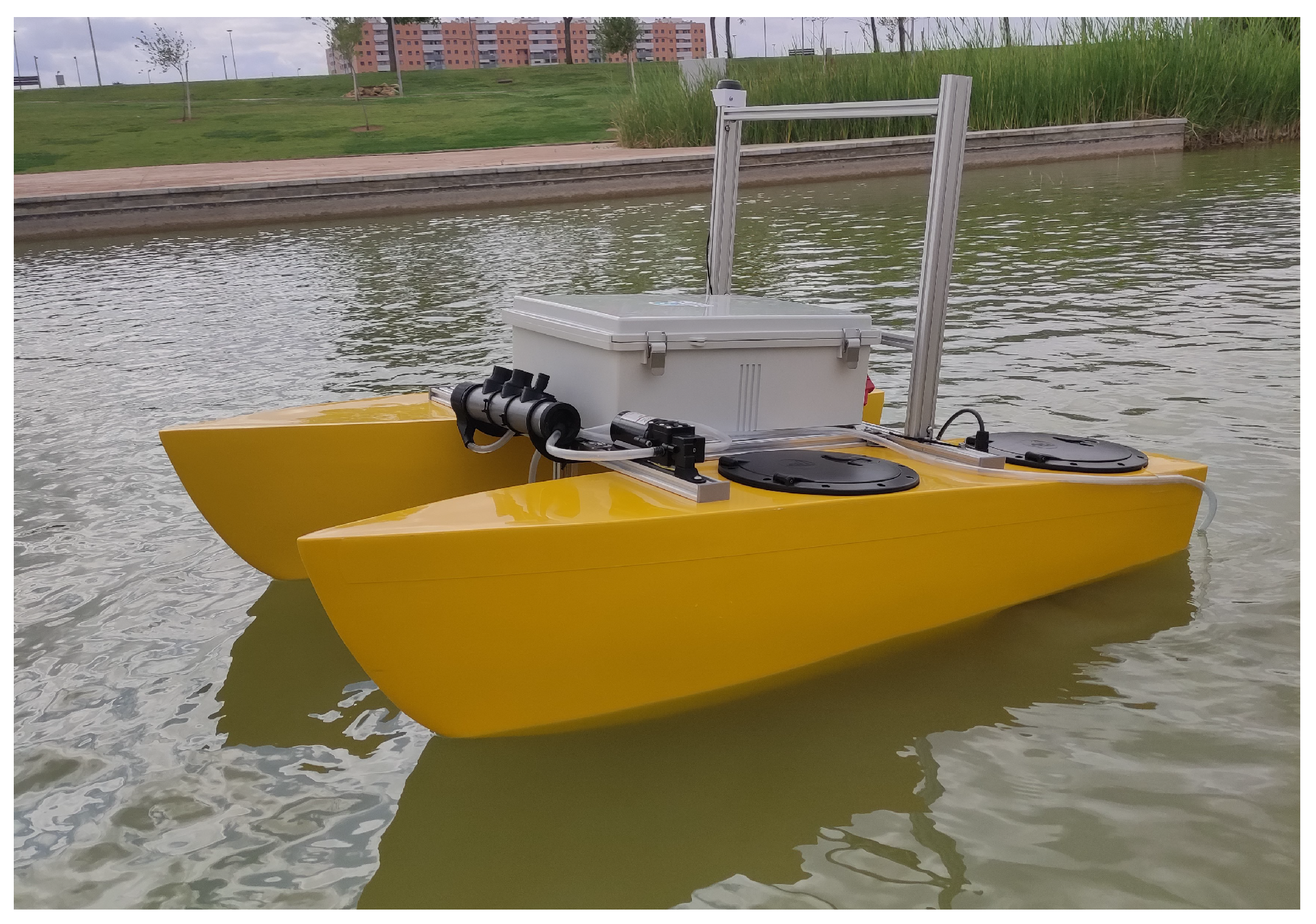
1], will not be efficient either due to the large surface area of the lake. In addition, the data provided do not generate a real model of the conditions of the lake water. In contrast, implementing a monitoring system using Autonomous Surface Vehicles (ASVs) (Figure 1), as in [1,2], will reduce human intervention, cost, and time spent for collecting data [3]. This monitoring system consists of deploying an ASV or a fleet of ASVs equipped with water quality sensors, in a water body, incorporating a guidance, navigation and control (GNC) system to guide the vehicles across the water surface.
GNC systems allow ASVs to move from one point to another on a determinate path autonomously. In the guidance system, the paths to be followed by the vehicles are generated. They can be generated by a global path planner, which creates an initial path with previous information, and a local path planner, which adapts the trajectories planned by the global planner with environmental information [4]. In a simple monitoring task, the data collected by the ASVs are not used to recalculate the path; the vehicles only travel through a defined path [5]. In contrast, an informative global path planning algorithm [6] generates an optimal path for the monitoring of the water resource and develops a model based on machine learning (ML) with the intention of estimating the state of the water body.
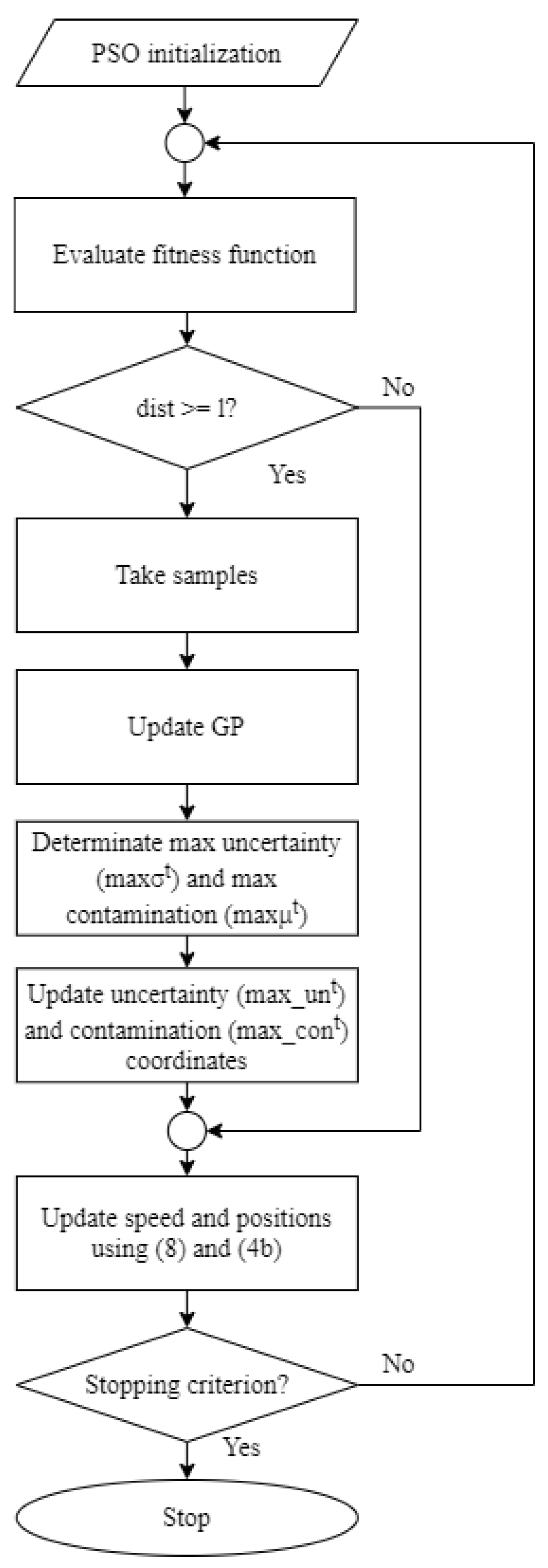
This work seeks to make up for the deficiency of simple monitoring tasks by implementing an informative path planning, an adapted version of a Particle Swarm Optimization (PSO) algorithm [7] with a Gaussian Process (GP) [
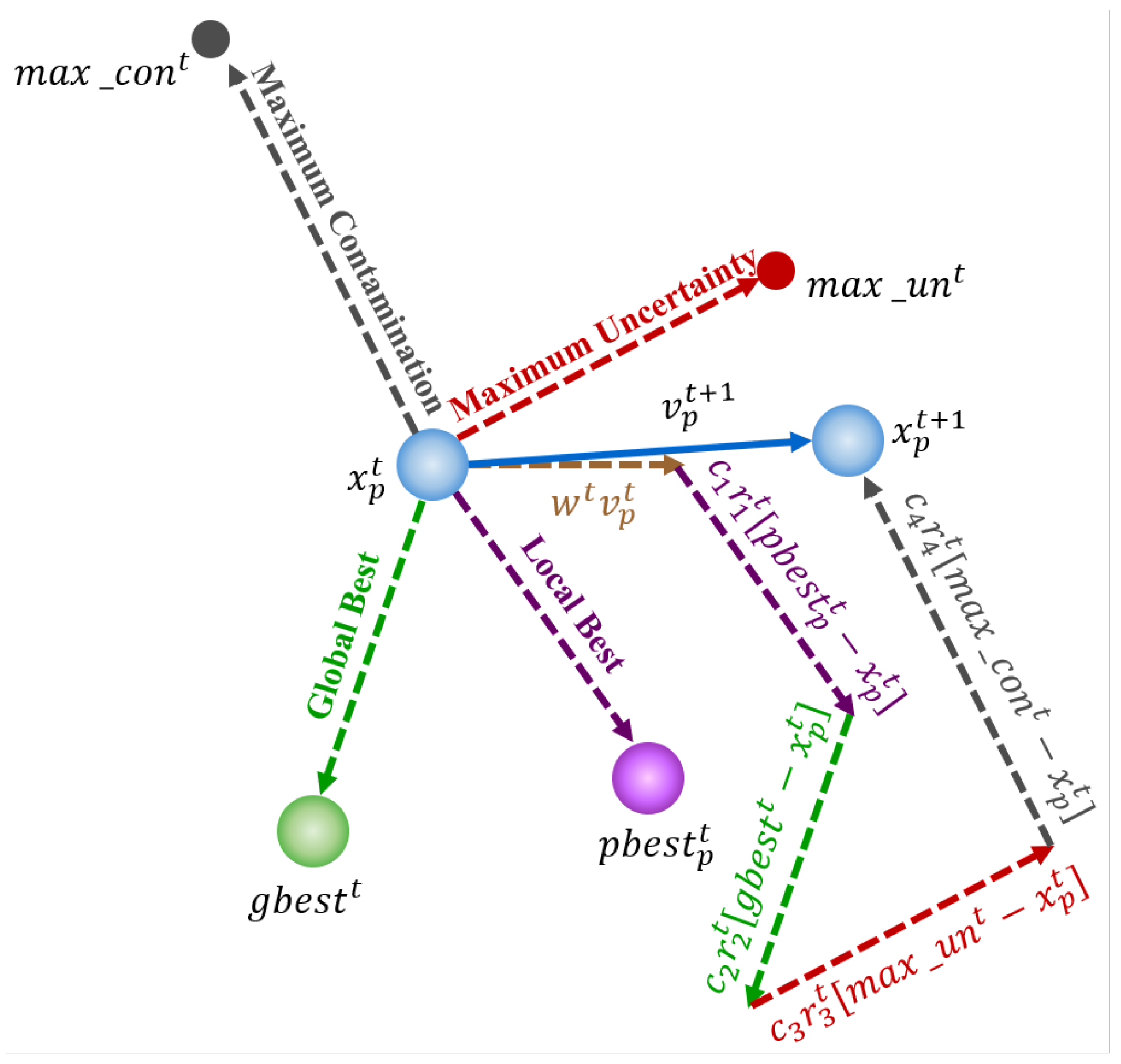
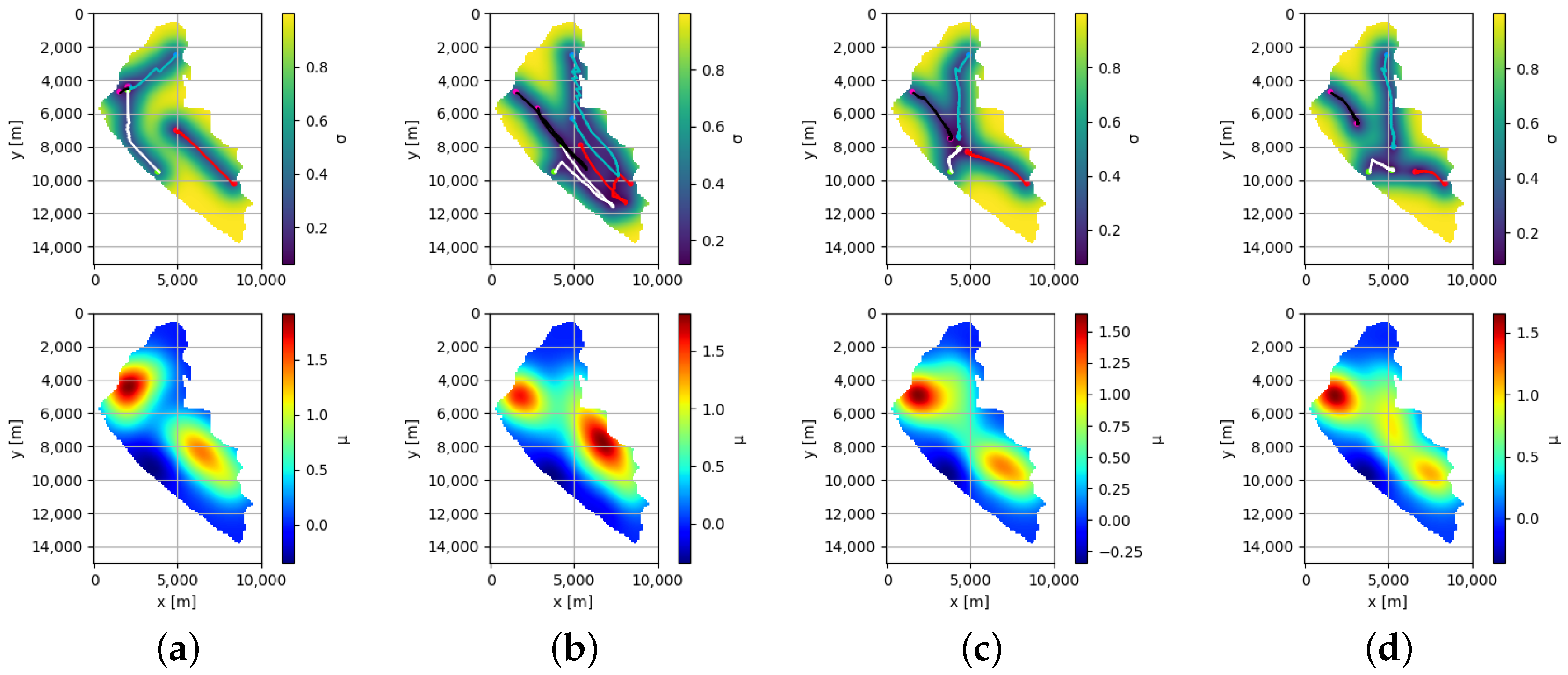
8], as an underlying surrogate model. Each of the ASVs from the fleet is represented by a particle of the swarm. With the proposed algorithm, the movements of the ASVs are determined by the model given by the GP, and also by the parameters of the PSO algorithm. After a certain distance traveled by the ASVs, data is collected, and the GP is updated accordingly. To explore the surface of the water resource, the uncertainty of the GP model is used, and to exploit areas with high contamination levels, the mean of the surrogate model is considered. The objective of the proposed approach is to obtain a suitable regression model of contamination levels of water resources in a limited time. Using the mean of the surrogate model, Ypacarai Lake as ground truth, and the considerable reduction in monitoring time are the main differences between the present work and the previous one [9].
The main contributions of this paper are:
  • The development of an informative path planner for a swarm of ASVs for the monitoring system of a water resource based on an improved meta-heuristic algorithm, PSO, with a GP as the underlying surrogate model.
  • The application of the proposed path planning using as the simulated scenario Ypacarai Lake, showing the superiority of the proposed approach with respect to other techniques.
This paper features the following sections: Section 2 contains several relevant works related to the proposed approach. Section 3 includes the statement of the problem and the main assumptions considered solving the monitoring problem. In Section 4 the proposed approach, based on PSO and GP, is described. Section 5 contains the simulation results obtained to validate the system. Section 6 includes the conclusions and future works. Finally, Appendix A, shows some obtained results of hyper-parameter optimization.

2. Related Works

Autonomous vehicles, both aquatic and aerial, have been the subject of extensive research in the previous decade [10]. Within the applications of autonomous vehicles, monitoring of water resources can be found [1,11,12]. The task is carried out by equipping an ASV with water quality sensors. To guide the vehicles, in [1], the authors propose an offline path planning of an ASV using a meta-heuristic technique, Genetic Algorithm (GA), and model the monitoring problem as the classical Travelling Salesman Problem (TSP). The main objective of the proposed offline path planning is to maximize the coverage of the surface of Ypacarai Lake. For this reason, a set of beacons located at the coast of the lake was considered. In [13], the authors extend the previous work, the main difference lies in the model of the monitoring problem, the problem is modelled using the Chinese Postman Problem (CPP). The CCP allows the planning of a path that repeats the visit to the beacons of the graph, different from TSP. As a result, the distance traveled by the ASV and the covered area increase its values. Furthermore, in [2], the authors combine exploration and intensification capabilities of their approach by online learning of the scenario. A global path planning is developed in [11] using Deep Reinforcement Learning (DRL). The authors model the monitoring problem as a Markov Decision Process, the states are represented as an RGB image of Ypacarai Lake and the potential positions of the ASV are the actions. In a more recent work [3], the authors work with multiple agents and the strategy applied was a centralized approach. In [14], the authors compare the performance of the Evolutionary Algorithm (EA) and deep reinforcement learning methodologies as monitoring systems. The results demonstrate the efficiency of the DRL technique under high-resolution conditions. The EA, on the other hand, delivers better results with lower resolution scenarios. Furthermore, the number of required hyper-parameters differs for each methodology; the evolutionary method requires few hyper-parameters to achieve a stable operation, whereas the DRL requires many. In addition, the DRL shows a high sensibility with respect to some hyper-parameters. However, DRL outperforms for the non-homogeneous patrolling problem for higher resolution scenarios, which demonstrates that the DRL methodology is more suitable as the complexity of the problem increases.
Bio-inspired techniques have been mainly employed as path planners and monitoring algorithms for water resources [15]. Bio-inspired techniques based on Swarm Intelligence (SI) have the advantage of working with several agents/particles simultaneously. Another advantage of SI is to efficiently solve nonlinear real world problems [16]. For path planning, algorithms as Ant Colony Optimization (ACO) [17,18], Bat Algorithm (BA) [19,20], Firefly Algorithm (FA) [21,22], and PSO [23,24], among others, can be used. In Table 1 is shown a comparison between some SI algorithms [25,26].
PSO algorithm is selected to be used in this work due to the easy implementation of the algorithm, the low number of parameters that must be adjusted and the large number of articles found where PSO and improved versions of PSO are applied to solve path planning problems for mobile robots and unmanned vehicles. In [23], three improved versions of PSO are proposed with the objective to enhance the robustness and avoid premature convergence. The strategies applied by the authors are the dynamic modification of the coefficients of PSO (inertia, local best and global best) and a random grouping inversion. The results demonstrate the effectiveness of the modifications, showing that by varying the coefficients and dividing the swarm into subgroups, the algorithm achieves better performance. In [24], the authors apply the Chaotic and Share-learning Particle Swarm Optimization (CSPSO) to solve the TSP problem and multi-objective path control. The algorithm is employed for marine environments and, in addition to improve the PSO algorithm, two-level collision avoidance rules and the impact of currents are provided. The PSO technique can also be combined with Elite Group-based Evolutionary Algorithms (EGEA), as in [27]. In EGEA, each individual of the evolutionary algorithm is capable to create its own groups of new solution. Afterward, according to the method, the individual with the best new solution of each group (Group Individual Elitist Selection (GIES)) or the best individuals in the whole group (Whole Population Elitist Selection (WPES)) are selected to the next generation. Based on the results, the best method for the PSO algorithm is the GIES. The reason for this is the influence of the best local of the particle. With the WPES method, particles with poor solutions are discarded and, as a result, huge changes are constantly made and the particle cannot maintain its best position, instead of the GIES method, which helps the selection of the best child of each particle.
A suitable path for monitoring systems can be generated using the data collected by the sensors. However, the collected data must be of high-quality. This problem is known as Informative Path Planning (IPP) problem [28]. Several approaches based on heuristics and approximation techniques have been proposed to solve this problem [29]. Informative Path Planning (IPP) techniques based on GP have been used to maximize the information collected by sensors [12,30]. Bayesian optimization (BO) based path planning with GP as underlying surrogate model is proposed in [12]. The authors present an analysis regarding the main components of the strategy, the acquisition functions (probability of improvement, expected improvement, scaled expected improvement, etc.) and the kernel (constant, radial basis function, Matérn, among others). Moreover, new adaptations of the classical methods of the acquisition functions are developed to improve the monitoring task of an ASV. An extension of this work can be found in [31], where the authors improved the monitoring system by adding a fusion of acquisitions functions. The purpose of the modification is that, when several water quality parameters are considered, a multi-function estimation scenario is generated due to different acquisition functions obtained. In [5], an online IPP framework is proposed. The authors use a sparse GP method to estimate sea surface temperature values. For the generation of the next point to visit, the path planning algorithm uses the variance in current prediction and remaining mission time. The results of the IPP are compared with the lawn mower paths. The IPP presents better match with the ground truth and lower root mean square error values than the lawn mower paths. IPP can also be used in aerial unmanned autonomous vehicles, as in [32], where the authors proposed two novel acquisitions functions for IPP with the objective of identifying anomalies in unknown environments.
In monitoring tasks, meta-heuristic algorithms such as GA [1,13] and PSO [23] try to maximize the covered area of the surface of water resources. However, these algorithms are unable to create a model of the water quality. Accordingly, a novel IPP is proposed in this work, combining meta-heuristic algorithm (PSO) with GP as surrogate model. In order to generate an optimal path to collect high-quality samples, the collected data is considered. By considering the collected data, the ASVs will be able to explore the water surface, by taking into consideration the uncertainty of the GP, and to exploit the sites with the highest levels of contamination, by weighting the movements of the ASVs with respect to the mean of the GP. Therefore, the proposed approach tries to balance adequately the mean and uncertainty of the GP in the monitoring task. Since the proposed approach incorporates up to four components (global best, local best, mean of the GP, and uncertainty of the GP) in the movement calculation of the ASV, suitable values for them should be selected. For this purpose, a BO-based hyper-parameter optimization will be applied. It uses prior information to obtain the parameter distribution, and it is widely used for machine learning models [33,34,35].

3. Statement of the Problem and Assumptions

This section describes the monitoring problem that an ASV fleet must address, as well as the key assumptions that were used to generate the simulated environment.

3.1. Monitoring Problem

The purpose of the monitoring system is to create a water quality model of water resources. To achieve the objective, the monitoring system consists of several ASVs equipped with water quality measurement sensors S. The real function of the water quality model can be represented as f ( x ) . The input of the function x is a location ( x , y ) in the water resource. A number of n measurements must be made by the ASVs in an environment in a sub-space of the R n space. The samples taken by the sensors are stored in a vector s = { s k | k = 1 , 2 , , n } , where the term k refers to the number of measures taken. In location q k , the ASVs perform the kth measurement. The vector q = { q k | k = 1 , 2 , , n } contains the locations of the ASVs. The vector D = { ( q k , s k ) | k = 1 , 2 , , N } corresponds to the data provided by the fleet of ASVs, the input vector x k is assigned to the locations of the vehicles q k , and the sensor read s k is assigned to the output value. Thus, the representation of each D k is
s k = f ( q k )
The Equation (2) represents the regression model that estimates the relation between the values of water quality y and the locations x in the entire domain of Ypacarai Lake
y f ( x ) ,
and, the real function f ( x ) can be approximated given enough data D.
The evaluation of the proposed approach is done using the Mean Square Error (MSE). In regression models, the MSE is usually used, for that reason, is a suitable metric for evaluating the model that has been obtained. The Equation (3) is used to calculate the MSE, where f ( x ) is the ground truth or real contamination map and y the resulting prediction of the surrogate model. The ground truth, in this work, is a distribution map of Ypacarai Lake.
MSE ( f ( x ) , y ) = 1 n samples k = 0 n samples 1 ( f ( x k ) y k ) 2
The monitoring system seeks to model the water quality of the lake as accurately as possible. Because of this, the metric used to evaluate whether the path is optimal is the Equation (3). That is, the closer the collected data is to the real data (low MSE), the better the generated path.

3.2. Assumptions

For the implementation of the proposed monitoring system, several assumptions are considered:
  • Ypacarai Lake: The model defined for the monitoring space is modelled as a matrix N , where each element N i , j has a value indicating the state of the grids. The matrix is composed by m × n squares of side d. If a square space is a natural obstacle, prohibited zone, land, among others, the square is painted white and has a value of 0, otherwise, the square is black and has a value of 1. Figure 2 shows the occupancy grid model of Ypacarai Lake used in the proposed approach. The ASVs are unable to move on land where the color of the square is white. For the simulations, the distribution map is scaled, each element N i j is 100 m × 100 m.
  • Coordinator: The system used for the fleet of ASVs is centralized. Therefore, the ASVs are linked to a global coordinator through the cloud, via 4 G or 5 G. In addition, it is considered a safety zone. For safety reasons, the ASVs are not allowed to travel near the shore of the lake. The distance considered is 2 squares of side d.
  • Sensors: The sensors that take the samples of the water quality parameters are considered ideal. As a result, the collected data by the ASVs are noiseless. As well, the GPS equipped in the ASVs are considered ideal, so there are no errors in the positions of the vehicles. The maximum speed of the ASVs is 2 m/s.
  • Navigation: The motions of the ASVs are error-free, and as a result, the traveled trajectories are faultless. Furthermore, obstructions and collisions are not taken into account.
  • Vehicle autonomy: Battery usage is deemed adequate for the duration of the test. The maximum distance traveled by the ASVs is approximately 20,000 m.

4. Proposed Approach

The main components and the functionality of the proposed methodology are described in this section. A review of the original PSO algorithm is performed first. Second, the underlying GP-based surrogate model that will be used to conduct the ASVs to high-uncertainty and high-contamination locations is outlined. Third, the proposed PSO for monitoring tasks is discussed. Finally, the hyper-parameter optimization that will be used is described.

4.1. Particle Swarm Optimization

PSO, proposed by [7], is a meta-heuristic optimization technique inspired in the social behavior of bird flocks. In PSO, each individual is referred to as a particle and represents a candidate solution for the optimization problem. Thus, a group of particles is called a swarm. Each particle moves around in multidimensional search-space, learning from their experience and from the other particles of the swarm. The velocity v i t + 1 and the position x p t + 1 of every particle p is updated at each iteration t according to the following equations:
v p t + 1 = w v p t + c 1 r 1 t pbest p t x p t + c 2 r 2 t gbest t x p t
x p t + 1 = x p t + v p t + 1
where w represents the inertia of the particle, pbest p t is the local best found by the particle (the optimal result of the particle), gbest t is the global best found by the swarm each time (the optimal result of the swarm). The terms v p t and x p t represents the speed and the position (coordinates ( x , y ) ) of the particle p at iteration t, respectively. The constants c 1 and c 2 are weights that determinate the importance of the local and global best components, known as acceleration coefficients. In other words, c 1 and c 2 are two stochastic acceleration components that guide the search toward optimum solution [7,36]. r 1 t and r 2 t are random values, in the range of [0, 1], that change their values at each iteration.

4.2. Gaussian Process Regression (GPR)

GP is based on multivariate normal distribution. As a result, the model can fit a set of points easily, each point represents a random variable. According to [37], GP is defined by a mean function and a covariance o kernel function. The main component is the kernel function, since, generally, the mean function is considered zero. The kernel is the function in charge of determining the expected shape, variability and smoothness of water quality variables that will be monitored in the proposed system. The selected kernel for the proposed approach is the Radial Basis Function (RBF) kernel, the reason is that in [12], by analyzing the different kernels, the results show that RBF is the most suitable kernel for aquatic environments.
In order to update the GPR, the input data D is marginalized and conditioned [37]. The Equation (5) is applied for the calculation of the unknown response of the GP ( μ ( x * ) , σ ( x * ) ).
μ f ^ ( x i ) * D = K * T K 1 f ( x )
σ f ^ ( x i ) * D = K * * K * T K 1 K *
From the fitted kernel K, K * * and K * are taken, where covariances between known data k ( x , x ) , unknown data k ( x , x ) and between both the known and unknown data k ( x , x ) are included
K = K K * K * T K * * = k ( x , x ) k ( x , x ) k ( x , x ) k ( x , x )

4.3. Monitoring System Based on PSO and GP

The main objective of the proposed approach is to overcome the limitations of the original PSO for the monitoring tasks and to improve the response time of the algorithm from the previous work [9]. This work proposes a path planning algorithm, where the uncertainty and the mean of the surrogate model is considered to guide the fleet of ASVs towards unexplored areas and zones with high contamination levels of the search space. In the PSO algorithm, the fleet is represented by a swarm and each ASV is considered a particle. The proposed approach does not take samples of the water at each iteration of the PSO, it only collects data after the distance traveled d i s t between the current location of the ASVs ( x t ) and the last location where the samples have been taken ( x sample ) is equal or greater than l:
l = λ × t
where λ is a ratio of one of the different length scales and t refers to the posterior length scale of the surrogate model [31]. This condition is applied to enhance the method provided in [9] in terms of simulation time by minimizing the quantity of data collected. By decreasing the amount of data, the GP does not need to update each iteration of the PSO, drastically decreasing the execution time of the monitoring system.
The pseudo-code of the proposed approach is shown in Algorithm 1 and the flowchart of the proposed approach is shown in Figure 3. At the beginning, the performance of the system is like the original PSO, since the initial values of the terms c 3 and c 4 (Figure 4) are set to 0. After the distance l is reached, the system takes samples of the water, the surrogate model is updated, and the GP calculate the maximum uncertainty and the maximum mean of the model to guide the movements of the swarm. The speeds of the ASVs is updated according to Equation (8) and the positions of the ASVs is updated according to Equation (4b).
v p t + 1 = w t v p t + c 1 r 1 t [ pbest p t x p t ] + c 2 r 2 t [ gbest t x p t ] + c 3 r 3 t [ max _ un t x p t ] + c 4 r 4 t [ max _ con t x p t ]
Algorithm 1: Enhanced GP-based PSO pseudo-code.
Electronics 10 01605 i001
The coordinates of the maximum uncertainty m a x σ t is represented by the term max _ un t and the term max _ con t represents the coordinates of the maximum mean of the model m a x μ t . Similar to c 1 and c 2 , the coefficients c 3 and c 4 are two stochastic acceleration components that guide the search toward areas with high uncertainty and areas with high levels of contamination, respectively. These four coefficients have to be tuned. Furthermore, Figure 4 illustrates the components of the speed vector of ASVs.
In Algorithm 1 and in Figure 3, d i s t total is the average distance traveled by each vehicle p from the initial location to the current location and d i s t sample is the average distance traveled from the initial location to the location where the last sample was taken. The number of iterations to be performed is represented by I.
In addition to the GP-based enhancements, the inertia is modified. The objective is the exploration and exploitation of the surface of the lake. Applying the Equation (9), at the beginning, the ASVs will focus on the exploration and, as iteration increase, the ASVs will focus on local exploitation of the lake [23].
w t = w m a x t ( ( w m a x w m i n ) / I )

4.4. Hyper-Parameter Optimization

In order to obtain a good performance of the proposed approach, several hyper-parameters have to be fine-tuned; the PSO hyper-parameters, c 1 , c 2 , c 3 and c 4 ; the GP length scale ; and the ratio λ . Fine-tuning hyper-parameters manually is tedious and time-consuming. In addition, this does not guarantee that the best values are obtained. Consequently, hyper-parameter optimization has been proposed by numerous researchers, for meta-heuristics algorithms [38,39], evolutionary algorithms [33], and neural networks [40], among others. Hyper-parameter optimization has the following advantages [41]: (i) Human effort is reduced, (ii) the algorithm has a better performance, and (iii) experiments with machine learning are more effective. Motivated by these reasons, hyper-parameter optimization has been applied in this work. The technique selected to perform the tuning is the BO.
According to [34], BO is an optimization algorithm very effective to solve tuning tasks and can be applied in functions difficult to compute, in functions that the difficulty to analyze their derivatives is high or in non-convex functions. Applying the Bayes theorem (10), the algorithm combines previous information of the unknown function, with data information, G, this allows to acquire the posterior of the function:
P ( F | G ) = P ( G | F ) × P ( F )
where P ( F | G ) is the posterior probability of the model F, P ( G | F ) is the likelihood of overserving G given model F, and P ( F ) is the prior probability.
BO optimizes a function using a surrogate model, which, considering the information provided by the evaluated points, is updated [33]. In order to balance the exploration and the exploitation in the selection of the next point to examine, acquisition function is used (Probability of improvement (PI) [42], Expected improvement (EI) [43], GP upper confidence bound (GP-UCB) [44]). For a detailed analysis of BO-based hyper-parameter optimization, readers are referred to [33,34,35]. According to the results provided in [34], EI and GP-UCB functions are faster than PI, and EI is less complicated than GP-UCB since there are no hyper-parameters that need to be tuned in EI as in GP-UCB. For these reasons, EI will be used in this work.

5. Performance Evaluation

In this section, the parameters used in the simulations are described, as well the results of the simulations are presented and discussed.

5.1. Simulation Setup

In this subsection, the ground truth and the simulation parameters are defined.

5.1.1. Ground Truth

The designed algorithm is available at https://github.com/MicaelaTenKathen/EGPPSO_ASV.git (accessed on 3 July 2021) and has been developed in Python using Scikit-learn (https://scikit-learn.org/stable/, accessed on 3 July 2021), DEAP (https://deap.readthedocs.io/en/master/, accessed on 3 July 2021) and Bayesian optimization (https://github.com/fmfn/BayesianOptimization, accessed on 3 July 2021) modules. The ground truth is a representation of Ypacarai Lake. The matrix N has a dimension of 100 px × 150 px, where each element N i j is 100 m × 100 m. For the distribution map of the water quality parameter, a benchmark function will be used, the Shekel Function (SF) (Equation (11)). The SF has the advantage of being a multidimensional, multimodal, continuous, and deterministic function [31].
f Shekel ( x ) = i = 1 M 1 c i + j = 1 N ( x j a i j ) 2
The function has two arguments, a i j and c i , that allows to specify several maximum locations. The elements a i j are located in matrix A, which has a size of M × N , where M denotes the number of maximum points and N denotes the space dimensions. The inverse significance value of the maximal locations is defined by matrix c, whose elements are c i and the size is M × 1 . In this work, N is set in 2, multiple simulations will be performed with different values of M in range of [2, 5], and the elements of c will have the same value. In order to validate the proposed approach, the monitoring system is tested using ten different ground truths generated by Equation (11) and pre-processed to fit the Ypacarai Lake. Examples of ground truths are shown in Figure 5. The maximum locations can be in restricted zones.

5.1.2. Simulation Parameters

For the mission, four ASVs are considered. Each vehicle must travel at least 15,000 m (scaled) to ensure effective monitoring. Therefore, the number of iterations is set to 6000, where d i s t t o t a l 17,000 m of each ASV. The maximum speed of the ASVs will be 2 m/s in the simulations.

5.2. Hyper-Parameter Optimization

Before simulating the monitoring system, fine tuning of the hyper-parameters must be performed. BO is used for this purpose, recall that EI is the selected acquisition function, as described in Section 4.4. Considering Table A5, in Appendix A, the RBF with length scale equal to 1.0 is used as the GP kernel. Additional settings that must be established in the Bayesian optimization module are the number of iterations of the BO and the initial points. The number of iterations is set as 20, and it is considered 10 random points as initial points. The hyper-parameters to be adjusted, and their respective bounds are shown in Table 2.
The range of the hyper-parameters of the PSO (the coefficient acceleration of the local best, c 1 ; the coefficient acceleration of the global best, c 2 ; the coefficient acceleration of the maximum uncertainty, c 3 ; and the coefficient acceleration of the maximum contamination, c 4 ) are specified according to [36,45]. To limit the range of values of the length scale of the GP, , the previous work is taken into account [9]. The results provided in [31] demonstrate that the monitoring system performs better if the ratio of the Equation (7), λ , is in the range of [ 0 , 0.5 ] . However, one of the main objectives of this work is to improve the simulation time of the algorithm, consequently, the range for λ is set to [ 0.1 , 0.5 ] , since, if λ = 0 , the algorithm will take data in each PSO iteration, increasing the execution time.
The proposed approach is simulated on 10 ground truths (cases). To obtain the optimal algorithm performance, the hyper-parameters must be optimized for each case. The values of the hyper-parameters in Table 3 are calculated in two ways: (i) The first optimization is the tuning performed specifically for each case (Case 1 to Case 10) (best of each ground truth); and (ii) the second optimization is the tuning using all cases (best of the whole group). In other words, in (i) for each case, only the MSE of that case is considered in the iterations of the BO, and in (ii), in each iteration of the BO, the mean of the MSE of all the cases in the Table 3 are considered (Case 1 to Case 10). Hyper-parameters are optimized with these two ways in order to compare the performance of the algorithm using the values of the best of each ground truth and the best of the whole group. The values obtained with BO, for a configuration of initial points, are shown in the Table 3.
These values are not suitable for all scenarios since they depend on the initial configuration, the number of iterations of the BO, the kernel used as shown in Table A1 and Table A3, included in Appendix A. These tables correspond to the hyper-parameter optimization applying Matérn ( n u = 2.5 , = 1.0 ) and RBF ( = 0.4 ) as kernel, respectively. In Table A5, in Appendix A, the mean of the MSE and the variability, of all cases (Case 1 to Case All), of the optimization of hyper-parameters with the different kernels used are shown. The comparison between the MSE and the average distance traveled of each ASV of the best hyper-parameters values for each case and the best hyper-parameters for the whole group are shown in Table 4.
The obtained results reveal that the MSE of simulations performed using the best of each case is lower than the simulations performed using the best hyper-parameters values of the whole group, which is to be anticipated given that the goal is to reduce the error for each ground truth. However, in some cases, there is not a significant difference in the MSE. In Figure 6, the results for two ground truths are shown. The figures at the top represent the movement of the ASVs and the uncertainty in the exploration of the lake surface. The trajectory of each one of the four ASVs is represented by lines of different colors. The water quality models generated by the enhanced GP-based PSO are shown at the bottom. The first two graphs (Figure 6a,b) correspond to the same ground truth (Case 4) and the last two belong to Case 9 (Figure 6c,d). The simulations Figure 6a,c are carried out with the best hyper-parameters values of each case (Case 4 and Case 9), and Figure 6b,d are carried out with the best hyper-parameters values for the whole group (All). The generated water quality models are similar to their respective ground truths, demonstrating a good performance of the proposed algorithm.

5.3. Comparison with Other Algorithms

After optimizing the hyper-parameters of the proposed approach, the performance of the original PSO [7], the GP-based PSO [9] and the enhanced GP-based PSO are compared. For the simulation of the three algorithms, the following adjustments are made: (i) The number of iterations has remained constant as 6000; (ii) the original PSO and the GP-based PSO collect data after some distance l (Equation (7)) is reached; (iii) case 0 is used as ground truth, therefore, the best hyper-parameter values for this case are considered; (iv) the hyper-parameters of the three algorithms are set to identical values (best values for case 0). Regarding the second adjustment, this condition is applied due to the excessive amount of time it would take for these algorithms to perform a simulation with 6000 iterations (about more than a week running on an Ubuntu server with 2.24 GHz AMD 16-Core Processor and 64 GB RAM), because in each iteration of the PSO, the GP is updated. The enhanced GP-based PSO performs 6000 iterations in approximately 120 s. Besides, performing simulations with only 200 iterations, as it is done in [9], is not efficient considering the dimensions of the map and the speed of the ASVs. Considering the third adjustment, in several cases of hyper-parameter optimization (Table 3), one of the c has a value equal to 0, so the influence that each term of Equation (8) has on the behavior of the proposed approach, it will not be able to be observed. However, in Case 0, all c have values greater than 0, allowing to observe the differences between the three algorithms when c 3 and c 4 are equal to 0 in the original PSO, and c 4 equal to 0 in the GP-based PSO. The settings for the simulations are summarized in Table 5.
In addition to the values set for the proposed approach shown in Table 5, a fourth simulation is made using the values of the best hyper-parameters values for the whole group in the enhanced GP-based PSO.
The Figure 7 shows the simulation of the monitoring system using the three algorithms. At the top, the movements of the ASVs are visualized, as well the uncertainty in the exploration of Ypacarai Lake. Each colored line represents an ASV trajectory. At the bottom, the water quality model generated by the surrogate model is shown. The Figure 7a represents the monitoring system using the original PSO. As the performance of the algorithm is based on the best local and the best global, the ASVs go towards one of the maximum peaks of the ground truth and the vehicles get stuck on a local optimum. On the other hand, using the GP-based PSO for the monitoring system (Figure 7b), the ASVs further explore the surface of the lake, oscillating between maximum points of uncertainty. When using the enhanced GP-based PSO for the monitoring of the lake (Figure 7c,d), the vehicles explore the surface until they reach a point where they exploit it. This action is a consequence of c 3 and c 4 , the greater one of the coefficients of acceleration is, the more the ASVs explore or exploit since terms 4 and 5 of Equation (8) focus on opposing objectives. The difference between Figure 7c,d are the values of the hyper-parameters. In Figure 7c the values are set as the Table 5 and in Figure 7d, the values are set as Case All (Table 3).
Comparing the obtained water quality models, the model generated by the GP-based PSO is closer to the greatest peaks of the ground truth. Instead, observing the scale of the graph, the first model estimated by the enhanced GP-based PSO achieves the minimum value of the water quality parameters, thereby reaching the ground truth. The average distance traveled by the ASVs with the original PSO is approximately 12,190 m. The reason for the short distance traveled is that the ASVs get stuck in a local optimum. The ASVs travel an average distance of 17,769 m when using the GP-based PSO, 17,937 m when using the enhanced GP-based PSO (Case 0) and 17,829 m when using the enhanced GP-based PSO (Case All).
The Figure 8a,b show the comparison of the three algorithms, the original PSO, the GP-based PSO and the enhanced GP-based PSO. However, in the Figure 8a,b is zoomed to the last three intervals so that the mean of the MSE and the range of variability of each algorithm can be differentiated. To obtain the mean of the MSE with its 95% confidence interval, 30 initial points configurations of the ASVs are considered, and the ground truth selected is the Case 0. The mean and standard deviation values have been computed using intervals in the range [0, 6000] in steps of 400 since the quantity of data obtained in the tests varied. The mean of the MSE of the algorithms fluctuates with time, as seen in Figure 8. At the beginning, the original PSO has the highest value of the mean of the MSE and the enhanced GP-based PSO (Case All) has the highest variability. Higher values of variability are due to the number of samples, by taking more samples, the variability will decrease. As the number of iterations increase, the mean of the MSE of the original PSO is the lowest of the three, while the mean of the GP-based PSO is the greatest. After 6000 iterations, the enhanced GP-based has the best mean of MSE and the lowest variability as shown in Table 6.

Discussion of the Results

The main results of this work are discussed below:
  • The proposed enhanced GP-based PSO considers not only the area with the highest uncertainty (unexplored areas) of the lake surface like in [9], but it also considers the area with the highest contamination to carry out the monitoring task.
  • The enhanced GP-based PSO is an algorithm capable to be used in any water resources. The proposed approach based the path generation in the samples that is collected from the surface of the water. As a consequence, the algorithm does not need to have more information about the environment than the data collected by the sensors. In addition, it is not necessary to perform previous calculations to generate an optimal path.
  • To improve the simulation time of our previous work, data is collected from the sensors and the surrogate model is updated only after the ASVs have traveled a distance l. With this improvement, the algorithm is capable of performing 6000 iterations in approximately 120 s.
  • To obtain the most suitable values for the enhanced GP-based PSO, a tuning has been carried out. The algorithm used for the hyper-parameter optimization is the BO and as acquisition function the EI is used. For kernel selection, three functions were tested, the Matérn ( n u = 2.5 , = 1.0 ) , the RBF ( = 1.0 ) , and RBF ( = 0.4 ) . The function that obtained the best MSE was the RBF ( = 1.0 ) , therefore, it is used for the tuning task.
  • With the hyper-parameter values obtained from the BO, the performance of three algorithms, the original PSO, the GP-based PSO and the enhanced GP-based PSO, were compared. The results showed that the proposed approach has the best MSE, being approximately 7 % lower than the MSE of the original PSO and 15 % lower than that of the GP-based PSO. Moreover, the enhanced GP-based PSO has the lowest variability of the three algorithms.

6. Conclusions and Future Works

An upgraded version of the GP-based PSO described in [9] is presented in this work. In a simulated scenario of Ypacarai Lake, four ASVs perform the monitoring mission. However, the proposed approach can be used in any scenario. In addition to exploring the surface of the lake, the vehicles exploit areas with high contamination levels. This can be achieved thanks to the uncertainty and the mean of the surrogate model. In order to validate the proposed approach, the Shekel function was used to model the water quality parameters of Ypacarai Lake. Before carrying out the simulations, the hyper-parameters were optimized using Bayesian optimization and considering 10 ground truths. After determining the optimal hyper-parameter settings, the performance of three algorithms was compared, the original PSO, the GP-based PSO and the proposed approach. The results show that the enhanced GP-based PSO, in simulation time, improves the GP-based PSO, performing simulations with 6000 iterations in a short time. In addition, it balances the exploration and exploitation of the surface of the lake. With the proposed algorithm, the best MSE values are obtained, which means that the generated path is optimal, since the generated model of the lake’s water quality is the most similar to the real model. As future work, the proposed algorithm will be compared with informative path planning algorithms designed for fleets or swarms of ASVs based on genetic algorithms, other swarm intelligence algorithms and/or Bayesian optimization, among other things. In addition, the algorithm is proposed to be improved by dynamically modifying the coefficient acceleration using deep reinforcement learning in such a way that the ASVs avoid getting stuck in a local optimum. Another improvement is to develop a monitoring system using a multi-objective PSO, considering several functions as water quality models at the same time. Each model could represent the data collected by a water quality sensor, such as pH, conductivity, temperature, etc.

Author Contributions

Conceptualization, D.G.R.; Methodology, M.J.T.K. and D.G.R.; Software, M.J.T.K.; Validation, M.J.T.K.; Formal analysis, M.J.T.K. and I.J.F.; Investigation, M.J.T.K. and D.G.R.; Data curation, M.J.T.K.; Writing—original draft preparation, M.J.T.K.; Writing—review and editing, I.J.F. and D.G.R.; Supervision, I.J.F. and D.G.R.; Project administration, I.J.F. and D.G.R.; Funding acquisition, D.G.R. All authors have read and agreed to the published version of the manuscript.

Funding

This work has been partially funded by the regional government Junta de Andalucía under the Projects “Despliegue Inteligente de una red de Vehículos Acuáticos no Tripulados para la monitorización de Recursos Hídricos US-1257508” and “Despliegue y Control de una Red Inteligente de Vehículos Autónomos Acuáticos para la Monitorización de Recursos Hídricos Andaluces PY18-RE0009”.

Data Availability Statement

The data that supports the results can be obtained using the scripts found in https://github.com/MicaelaTenKathen/EGPPSO_ASV.git (accessed on 3 July 2021).

Acknowledgments

This work was proofread by Federico Peralta and Samuel Yanes Luis.

Conflicts of Interest

The authors declare no conflict of interest.

Appendix A

In order to select the most suitable hyper-parameters for the proposed approach, three hyper-parameter optimization based on Bayesian optimization (https://github.com/fmfn/BayesianOptimization, accessed on 3 July 2021) was carried out. The difference between the three hyper-parameter optimization was the kernel used. The first kernel used was the Matérn ( n u = 2.5 , = 1.0 ) , this was due to default setting of the Bayesian optimization module, the results of this hyper-parameter optimization is shown in Table A1, and the MSE and the average distance is shown in Table A2. The second kernel used was the default setting of the Scikit-learn (https://scikit-learn.org/stable/, accessed on 3 July 2021) module, the RBF ( = 1.0 ) . The last kernel tested was the RBF ( = 0.4 ) . The reason was to compare the results between different values of . The results of the hyper-parameter optimization is shown in Table A3, and the MSE and the average distance is shown in Table A4. The values of MSE obtained with the second configuration was the best (Table A5). As a consequence, the values calculated with this kernel was used for the simulations, Table 3 and Table 4.
Table A1. Hyper-parameter optimization using Matérn ( n u = 2.5 , = 1.0 ) as kernel.
Case c 1 c 2 c 3 c 4 λ
12.69710.69362.66942.96810.55890.1
22.59661.47612.92412.469310.1
31.25400.57880.10102.61080.48260.1109
43.09622.66472.38320.53910.63680.1
53.66720.37843.94663.78800.67240.1053
61.82402.798101.04800.42020.1
72.06871.73962.56611.276610.1
82.18111.20991.63721.735010.1
91.16490.77470.03062.73620.40.1
102.32951.43522.17931.83420.87910.1
All3.46431.627900.98800.40.1
Table A2. Comparison of the MSE and the average distance using the values of Table A1.
CaseEach Ground TruthAll Ground Truths
MSEAverage Distance [m]MSEAverage Distance [m]
10.006217,0480.008716,860
20.007517,9190.007617,720
30.012317,9340.010717,862
40.011117,0630.014516,896
50.017617,6470.013916,861
60.003716,3820.003716,796
70.007117,0420.008616,661
80.008017,2740.009016,610
90.004216,9420.004516,705
100.002517,2810.002516,875
Table A3. Hyper-parameter optimization using RBF ( = 0.4 ) as kernel.
Case c 1 c 2 c 3 c 4 λ
12.58100.85813.34243.37200.40.1
21.95551.04622.60773.330410.1
32.26663.318001.09860.40.1
43.45342.84533.60831.72960.40.1
51.87512.776400.98600.40890.1
61.57532.705401.23120.65460.1
72.27770.46242.27283.343810.1
82.81310.83592.18282.48070.65010.1
90.27283.894903.53050.88920.1
101.91601.39011.53192.08150.58700.1
All2.75751.99451.98992.65700.98130.1
Table A4. Comparison of the MSE and the average distance using the values of Table A3.
CaseEach Ground TruthAll Ground Truths
MSEAverage Distance [m]MSEAverage Distance [m]
10.006217,0530.006817,047
20.007417,9200.007717,917
30.010717,7300.013517,920
40.010817,1570.012017,040
50.013816,8600.017317,416
60.003816,0810.005117,918
70.007417,0480.007917,044
80.008017,3480.008117,108
90.004216,9050.006417,115
100.002717,3060.002717,273
Table A5. MSE of the hyper-parameter optimization using different kernels.
KernelMSE (Each Ground Truth)MSE (All Ground Truths)
Matérn ( n u = 2.5 , = 1.0 ) 0.0080 ± 0.00460.0084 ± 0.0040
RBF ( = 1.0 ) 0.0071 ± 0.00340.0081 ± 0.0040
RBF ( = 0.4 ) 0.0075 ± 0.00350.0088 ± 0.0043
It is important to mention that, in the Case 3 and the Case 5 of Table A1, the MSE obtained using the best hyper-parameter values for these cases is higher than the MSE obtained using the best hyper-parameter values for the whole group. The reason is that, as it is an optimization problem, the function could get stuck in a local optimum. A solution can be increased the number of iteration of the BO. In Table A5, the mean of the MSE with its 95% confidence interval of the three hyper-parameter optimization is shown. The calculations were made considering the MSE of all the cases shown in the Table 4, Table A2 and Table A4, from Case 1 to Case All. The results show that the BO with RBF ( = 1.0 ) as kernel is the one with the best MSE, which is why it was used in this work.

References

  1. Arzamendia, M.; Gregor, D.; Reina, D.G.; Toral, S.L. An evolutionary approach to constrained path planning of an autonomous surface vehicle for maximizing the covered area of Ypacarai Lake. Soft Comput. 2019, 23, 1723–1734. [Google Scholar] [CrossRef]
  2. Arzamendia, M.; Reina, D.G.; Toral, S.; Gregor, D.; Asimakopoulou, E.; Bessis, N. Intelligent online learning strategy for an autonomous surface vehicle in lake environments using evolutionary computation. IEEE Intell. Transp. Syst. Mag. 2019, 11, 110–125. [Google Scholar] [CrossRef]
  3. Luis, S.Y.; Reina, D.G.; Marín, S.L.T. A Multiagent Deep Reinforcement Learning Approach for Path Planning in Autonomous Surface Vehicles: The YpacaraC-Lake Patrolling Case. IEEE Access 2021, 9, 17084–17099. [Google Scholar] [CrossRef]
  4. Peralta, F.; Arzamendia, M.; Gregor, D.; Reina, D.G.; Toral, S. A Comparison of Local Path Planning Techniques of Autonomous Surface Vehicles for Monitoring Applications: The Ypacarai Lake Case-study. Sensors 2020, 20, 1488. [Google Scholar] [CrossRef] [PubMed] [Green Version]
  5. Mishra, R.; Chitre, M.; Swarup, S. Online Informative Path Planning Using Sparse Gaussian Processes. In Proceedings of the 2018 OCEANS—MTS/IEEE Kobe Techno-Oceans (OTO), Kobe, Japan, 28–31 May 2018; pp. 1–5. [Google Scholar] [CrossRef]
  6. Bottarelli, L.; Bicego, M.; Blum, J.; Farinelli, A. Orienteering-based informative path planning for environmental monitoring. Eng. Appl. Artif. Intell. 2019, 77, 46–58. [Google Scholar] [CrossRef]
  7. Kennedy, J.; Eberhart, R. Particle swarm optimization. In Proceedings of the ICNN’95-International Conference on Neural Networks. IEEE, Perth, WA, Australia, 27 November–1 December 1995; Volume 4, pp. 1942–1948. [Google Scholar]
  8. Quiñonero-Candela, J.; Rasmussen, C.E. A unifying view of sparse approximate Gaussian process regression. J. Mach. Learn. Res. 2005, 6, 1939–1959. [Google Scholar]
  9. Jara, M.; Reina, D.G.; Jurado, I.; Tapia, A. Autonomous Monitoring System for Water Resources based on PSO and Gaussian Process. In Proceedings of the 2021 IEEE Congress on Evolutionary Computation (CEC), Kraków, Poland, 28 June–1 July 2021. in press. [Google Scholar]
  10. Sánchez-García, J.; García-Campos, J.M.; Arzamendia, M.; Reina, D.G.; Toral, S.L.; Gregor, D. A survey on unmanned aerial and aquatic vehicle multi-hop networks: Wireless communications, evaluation tools and applications. Comput. Commun. 2018, 119, 43–65. [Google Scholar] [CrossRef]
  11. Yanes Luis, S.; Reina, D.G.; Toral Marín, S.L. A Deep Reinforcement Learning Approach for the Patrolling Problem of Water Resources Through Autonomous Surface Vehicles: The Ypacarai Lake Case. IEEE Access 2020, 8, 204076–204093. [Google Scholar] [CrossRef]
  12. Samaniego, F.P.; Reina, D.G.; Marín, S.L.T.; Arzamendia, M.; Gregor, D.O. A Bayesian Optimization Approach for Water Resources Monitoring Through an Autonomous Surface Vehicle: The Ypacarai Lake Case Study. IEEE Access 2021, 9, 9163–9179. [Google Scholar] [CrossRef]
  13. Arzamendia, M.; Espartza, I.; Reina, D.G.; Toral, S.L.; Gregor, D. Comparison of eulerian and hamiltonian circuits for evolutionary-based path planning of an autonomous surface vehicle for monitoring ypacarai lake. J. Ambient. Intell. Humaniz. Comput. 2019, 10, 1495–1507. [Google Scholar] [CrossRef]
  14. Yanes Luis, S.; Gutiérrez-Reina, D.; Toral Marín, S. A Dimensional Comparison between Evolutionary Algorithm and Deep Reinforcement Learning Methodologies for Autonomous Surface Vehicles with Water Quality Sensors. Sensors 2021, 21, 2862. [Google Scholar] [CrossRef]
  15. Jahandideh-Tehrani, M.; Bozorg-Haddad, O.; Loáiciga, H.A. Application of particle swarm optimization to water management: An introduction and overview. Environ. Monit. Assess. 2020, 192, 1–18. [Google Scholar] [CrossRef]
  16. Yang, X.S.; Karamanoglu, M. Swarm intelligence and bio-inspired computation: An overview. Swarm Intell. Bio-Inspired Comput. 2013, 3–23. [Google Scholar] [CrossRef]
  17. Wang, H.J.; Fu, Y.; Zhao, Z.Q.; Yue, Y.J. An Improved Ant Colony Algorithm of Robot Path Planning for Obstacle Avoidance. J. Robot. 2019, 2019, 8. [Google Scholar] [CrossRef] [Green Version]
  18. Konatowski, S.; Pawłowski, P. Ant colony optimization algorithm for UAV path planning. In Proceedings of the 2018 14th International Conference on Advanced Trends in Radio elecrtronics, Telecommunications and Computer Engineering (TCSET), Lviv-Slavske, Ukraine, 20–24 February 2018; pp. 177–182. [Google Scholar]
  19. Ibraheem, I.K.; Ajeil, F.H.; Khan, Z.H. Path planning of an autonomous mobile robot in a dynamic environment using modified bat swarm optimization. arXiv 2018, arXiv:1807.05352. [Google Scholar]
  20. Zhou, X.; Gao, F.; Fang, X.; Lan, Z. Improved bat algorithm for UAV path planning in three-dimensional space. IEEE Access 2021, 9, 20100–20116. [Google Scholar] [CrossRef]
  21. Patle, B.; Pandey, A.; Jagadeesh, A.; Parhi, D.R. Path planning in uncertain environment by using firefly algorithm. Def. Technol. 2018, 14, 691–701. [Google Scholar] [CrossRef]
  22. Li, F.; Fan, X.; Hou, Z. A Firefly Algorithm With Self-Adaptive Population Size for Global Path Planning of Mobile Robot. IEEE Access 2020, 8, 168951–168964. [Google Scholar] [CrossRef]
  23. Xin, J.; Li, S.; Sheng, J.; Zhang, Y.; Cui, Y. Application of improved particle swarm optimization for navigation of unmanned surface vehicles. Sensors 2019, 19, 3096. [Google Scholar] [CrossRef] [Green Version]
  24. Guo, X.; Ji, M.; Zhao, Z.; Wen, D.; Zhang, W. Global path planning and multi-objective path control for unmanned surface vehicle based on modified particle swarm optimization (PSO) algorithm. Ocean. Eng. 2020, 216, 107693. [Google Scholar] [CrossRef]
  25. Selvi, V.; Umarani, R. Comparative analysis of ant colony and particle swarm optimization techniques. Int. J. Comput. Appl. 2010, 5, 1–6. [Google Scholar] [CrossRef]
  26. Abdmouleh, Z.; Gastli, A.; Ben-Brahim, L.; Haouari, M.; Al-Emadi, N.A. Review of optimization techniques applied for the integration of distributed generation from renewable energy sources. Renew. Energy 2017, 113, 266–280. [Google Scholar] [CrossRef]
  27. Xiong, C.; Lu, D.; Zeng, Z.; Lian, L.; Yu, C. Path Planning of Multiple Unmanned Marine Vehicles for Adaptive Ocean Sampling Using Elite Group-Based Evolutionary Algorithms. J. Intell. Robot. Syst. 2020, 99, 875–889. [Google Scholar] [CrossRef]
  28. Velasco, O.; Valente, J.; Mersha, A.Y. An Adaptive Informative Path Planning Algorithm for Real-time Air Quality Monitoring Using UAVs. In Proceedings of the 2020 International Conference on Unmanned Aircraft Systems (ICUAS), Athens, Greece, 9–12 June 2020; pp. 1121–1130. [Google Scholar]
  29. Choudhury, S.; Gruver, N.; Kochenderfer, M.J. Adaptive informative path planning with multimodal sensing. In Proceedings of the International Conference on Automated Planning and Scheduling, Nancy, France, 14–19 June 2020; Volume 30, pp. 57–65. [Google Scholar]
  30. Chauvin-Hameau, C.G.C. Informative Path Planning for Algae Farm Surveying. 2020. Available online: https://www.diva-portal.org/smash/get/diva2:1438452/FULLTEXT02.pdf (accessed on 3 July 2021).
  31. Peralta, F.; Reina, D.G.; Toral, S.; Arzamendia, M.; Gregor, D. A Bayesian Optimization Approach for Multi-Function Estimation for Environmental Monitoring Using an Autonomous Surface Vehicle: Ypacarai Lake Case Study. Electronics 2021, 10, 963. [Google Scholar] [CrossRef]
  32. Blanchard, A.; Sapsis, T. Informative path planning for anomaly detection in environment exploration and monitoring. arXiv 2020, arXiv:2005.10040. [Google Scholar]
  33. Roman, I.; Ceberio, J.; Mendiburu, A.; Lozano, J.A. Bayesian optimization for parameter tuning in evolutionary algorithms. In Proceedings of the 2016 IEEE Congress on Evolutionary Computation (CEC), Vancouver, BC, Canada, 24–29 July 2016; pp. 4839–4845. [Google Scholar]
  34. Wu, J.; Chen, X.Y.; Zhang, H.; Xiong, L.D.; Lei, H.; Deng, S.H. Hyperparameter optimization for machine learning models based on Bayesian optimization. J. Electron. Sci. Technol. 2019, 17, 26–40. [Google Scholar]
  35. Kim, Y.; Chung, M. An Approach to Hyperparameter Optimization for the Objective Function in Machine Learning. Electronics 2019, 8, 1267. [Google Scholar] [CrossRef] [Green Version]
  36. Ratnaweera, A.; Halgamuge, S.K.; Watson, H.C. Self-organizing hierarchical particle swarm optimizer with time-varying acceleration coefficients. IEEE Trans. Evol. Comput. 2004, 8, 240–255. [Google Scholar] [CrossRef]
  37. Williams, C.; Rasmussen, C. Gaussian Processes for Machine Learning; MIT Press: Cambridge, MA, USA, 2006; Volume 2. [Google Scholar]
  38. Birattari, M.; Kacprzyk, J. Tuning Metaheuristics: A Machine Learning Perspective; Springer: Berlin/Heidelberg, Germany, 2009; Volume 197. [Google Scholar]
  39. Lessmann, S.; Caserta, M.; Arango, I.M. Tuning metaheuristics: A data mining based approach for particle swarm optimization. Expert Syst. Appl. 2011, 38, 12826–12838. [Google Scholar] [CrossRef]
  40. Guo, B.; Hu, J.; Wu, W.; Peng, Q.; Wu, F. The tabu_genetic algorithm: A novel method for hyper-parameter optimization of learning algorithms. Electronics 2019, 8, 579. [Google Scholar] [CrossRef] [Green Version]
  41. Feurer, M.; Hutter, F. Hyperparameter optimization. In Automated Machine Learning; Springer: Cham, Switzerland, 2019; pp. 3–33. [Google Scholar]
  42. Kushner, H.J. A New Method of Locating the Maximum Point of an Arbitrary Multipeak Curve in the Presence of Noise. J. Basic Eng. 1964, 86, 97–106. [Google Scholar] [CrossRef]
  43. Mockus, J.; Tiesis, V.; Zilinskas, A. The Application of Bayesian Methods for Seeking the Extremum. Towards Glob. Optim. 1978, 2, 2. [Google Scholar]
  44. Srinivas, N.; Krause, A.; Kakade, S.M.; Seeger, M. Gaussian process optimization in the bandit setting: No regret and experimental design. arXiv 2009, arXiv:0912.3995. [Google Scholar]
  45. Senthil Arumugam, M.; Rao, M.; Chandramohan, A. A new and improved version of particle swarm optimization algorithm with global-local best parameters. Knowl. Inf. Syst. 2008, 16, 331–357. [Google Scholar] [CrossRef]
Figure 1. Autonomous surface vehicle using for the monitoring task.
Electronics 10 01605 g001
Figure 2. Model of the occupancy grid of Ypacarai Lake.
Electronics 10 01605 g002
Figure 3. Flowchart of the proposed approach.
Electronics 10 01605 g003
Figure 4. Components of proposed PSO.
Electronics 10 01605 g004
Figure 5. Example of 3 ground truths of the 10 simulated ground truths obtained with the Shekel function using the Ypacarai Lake as simulated scenario.
Electronics 10 01605 g005
Figure 6. Representation of movements of the ASVs and uncertainty in the exploration of the lake surface (top) and mean of the surrogate model (bottom) in two different ground truths.
Electronics 10 01605 g006
Figure 7. Representation of movements of the ASVs and uncertainty in the exploration of the lake surface (top) and mean of the surrogate model (bottom) using three different algorithms.
Electronics 10 01605 g007
Figure 8. MSE using the original PSO, the GP-based PSO and the enhanced GP-based PSO.
Electronics 10 01605 g008
Table 1. Comparison between SI techniques.
AlgorithmBiological MotivationAdvantagesDisadvantages
ACOAnt colonies- Effective in discovering good solutions.- Theoretical analysis is difficult.
- Adaptation to changes.- Research is more experimental than theoretical.
- Converge.- The convergence time is uncertain.
BAEcholocation of bats- Few parameters.- Can get trapped in multi-dimensional functions.
- Simple to implement.- If the dimensions of the problem increase, the chances of converging towards a global optimal solution decrease.
- Low accuracy.
FAFireflies attraction- Simple to implement.- Slow convergence.
- Parallel implementation.- Get easily stuck in local optimum for multi-modal problems.
- Do not save the best solutions.
PSOBird flocks- Simple to implement.- Get stuck in local optimum.
- Few parameters to be tuned.- Dispersion problems cannot be solved.
- Do not overlap or mutate- Initial design parameters can be difficult to define.
Table 2. Range for hyper-parameter optimization.
Hyper-ParameterRange
c 1 [0, 4]
c 2 [0, 4]
c 3 [0, 4]
c 4 [0, 4]
[0.4, 1.0]
λ [0.1, 0.5]
Table 3. Values of the hyper-parameter optimization using RBF ( = 1.0 ) as kernel.
Case c 1 c 2 c 3 c 4 λ
11.98570.86042.8352410.1
20.674103.44343.05030.68920.1
3400.04641.49280.51780.1
43.76482.25121.96760.15260.40.1
52.12252.723600.73530.40.1
61.81543.152300.62710.40.1
71.63202.67332.3820010.1
82.44013.56592.05320.10410.40.1
90.33393.871903.53020.86680.1
103.12862.5680.7900010.1
All41.08301.131600.40.1
Table 4. Comparison of the MSE and the average distance.
CaseEach Ground TruthAll Ground Truths
MSEAverage Distance [m]MSEAverage Distance [m]
10.006317,0420.006717,041
20.006717,9150.007318,094
30.008617,0330.011518,879
40.010917,0590.011017,193
50.013816,5740.016617,765
60.003815,9920.004917,956
70.006717,0420.007017,038
80.008016,7550.008117,542
90.004216,9010.005717,478
100.002217,0380.002517,563
Table 5. Simulations adjustments.
Parameter / Hyper-ParameterOriginal PSOGP-Based PSOEnhanced GP-Based PSO
Number of ASVs444
Maximum speed of the ASVs (m/s)222
Surface limits (m)x [0, 10,000]x [0, 10,000]x [0, 10,000]
y [0, 15,000]y [0, 15,000]y [0, 15,000]
Iterations600060006000
Ground truthCase 0Case 0Case 0
w1--
w m i n -0.40.4
w m a x -0.90.9
c 1 1.98571.98571.9857
c 2 0.86040.86040.8604
c 3 -2.83522.8352
c 4 --4
111
λ 0.10.10.1
Table 6. Comparison between the three algorithms.
AlgorithmMSEAverage Distance [m]
Original PSO0.0074 ± 0.006312,190
GP-based PSO0.0087 ± 0.004517,769
Enhanced GP-based PSO (Case 0)0.0069 ± 0.003317,937
Enhanced GP-based PSO (Case All)0.0074 ± 0.004517,829
Publisher’s Note: MDPI stays neutral with regard to jurisdictional claims in published maps and institutional affiliations.

