
Analysis of a Nonlinear Technique for Microwave Imaging of Targets Inside Conducting Cylinders


Abstract
:1. Introduction
2. Problem Formulation
Green’s Function of the Considered Problem
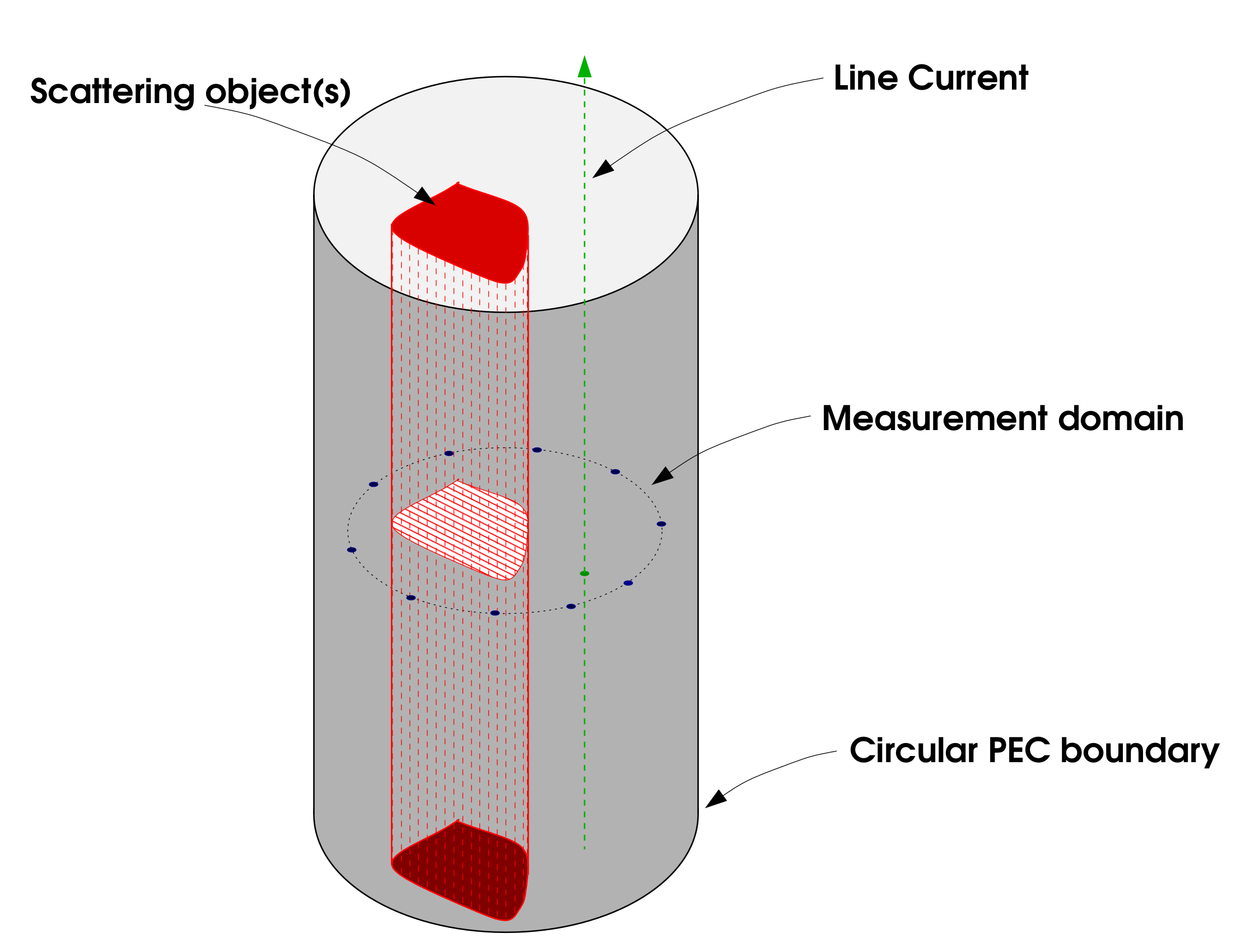
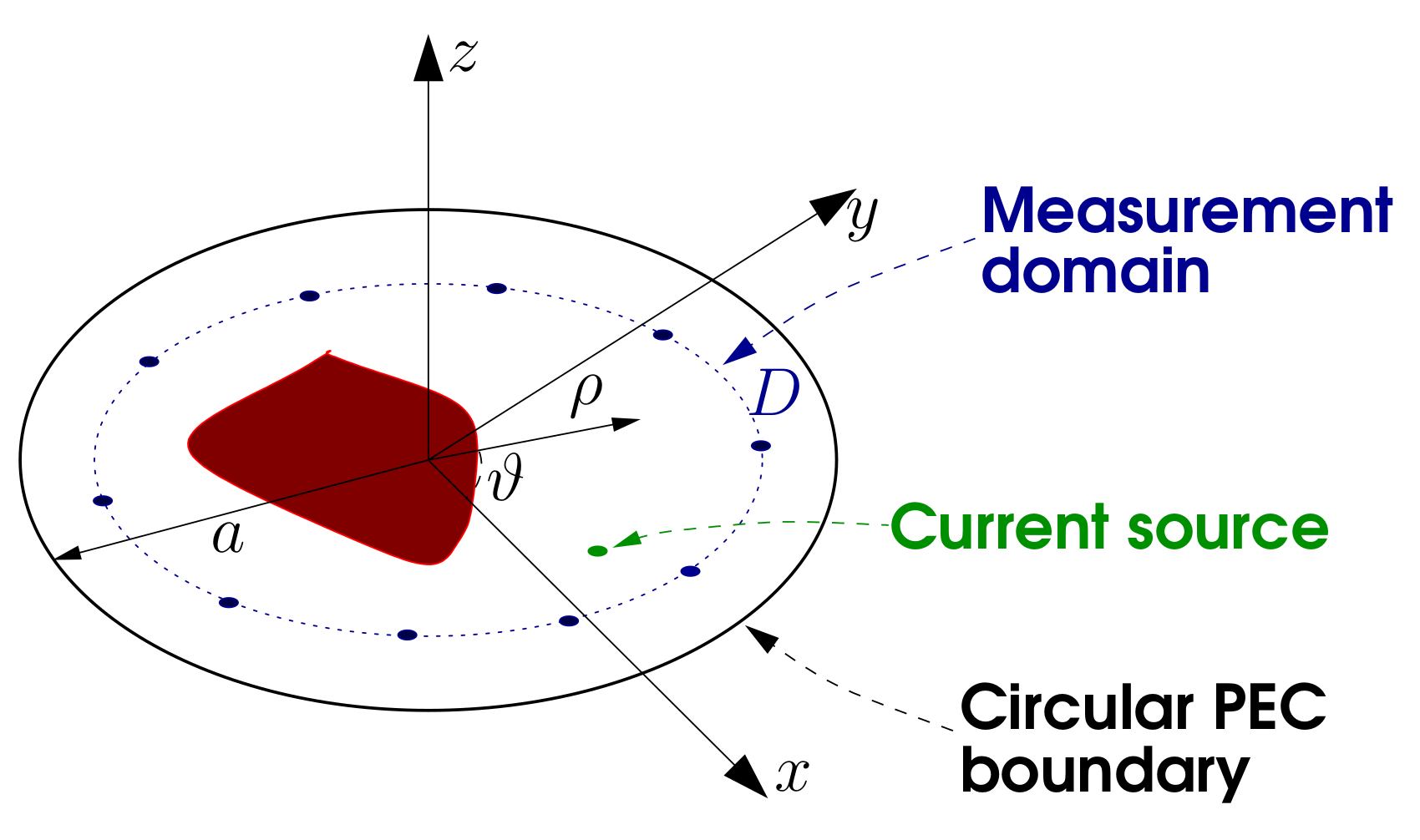
- while in free space the scattering field can be expanded into a simple sum of progressing waves, in the present problem the solution is made by a sum of complicated standing waves, and many resonant modes can arise inside the cavity;
- the incident field is also strongly affected by the cavity boundaries: while the line current produces a simple circular wave in free space, in the present problem the incident field has the same form of the Green’s function (compare Equations (2) and (6)), hence it contains many contributions, made of standing waves depending on the cavity dimensions.
- a.
- ;
- b.
- ;
- c.
- ;
- d.
- ;
- e.
- .
3. Nonlinear Inverse Scattering Method
4. Results of Numerical Simulations
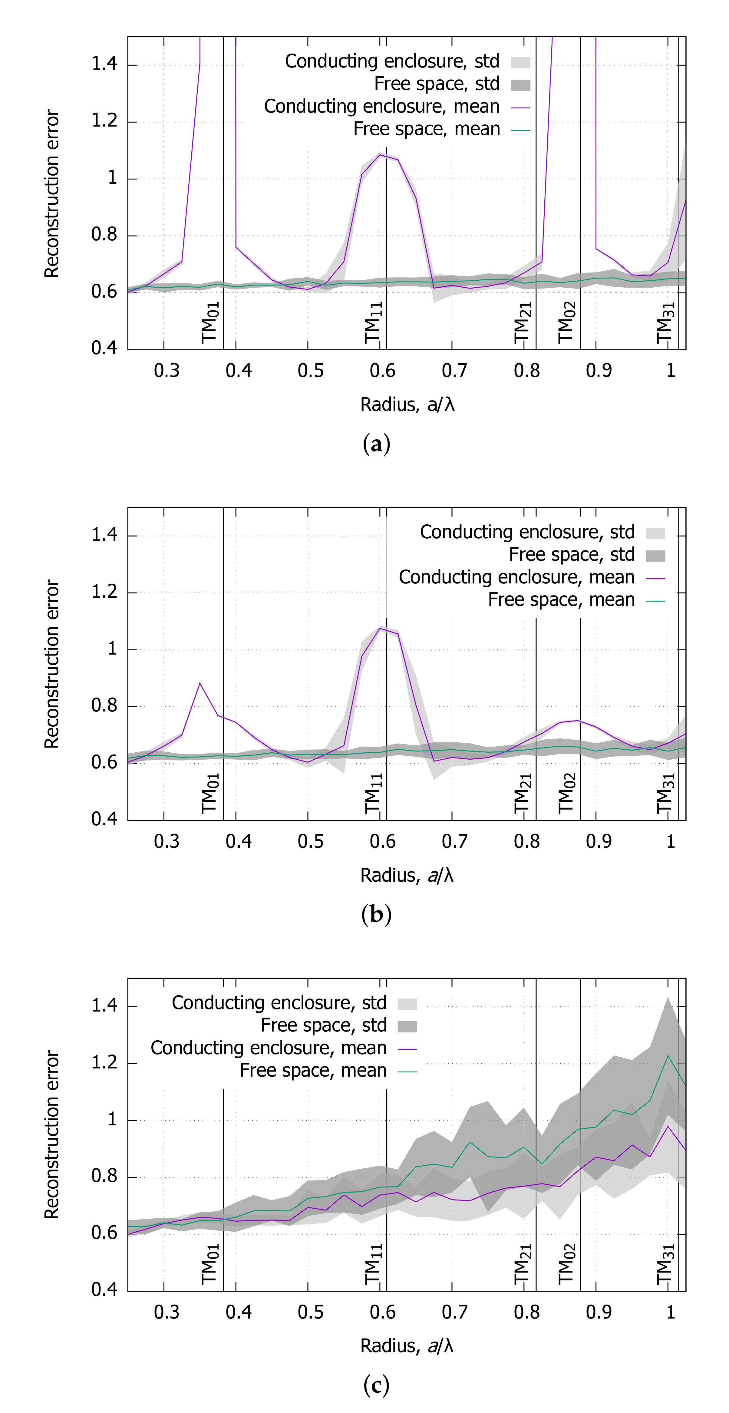
4.1. Small Conducting Enclosure
4.2. Large Conducting Enclosure
5. Conclusions
Author Contributions
Funding
Data Availability Statement
Conflicts of Interest
Abbreviations
| PEC | Perfect Electric Conductor |
| TM | Transverse Magnetic |
| Normalized Reconstruction Error | |
| RAM | Random Access Memory |
References
- Kak, A.C.; Slaney, M. Principles of Computerized Tomographic Imaging; IEEE Press: New York, NY, USA, 1988. [Google Scholar]
- Benedetto, A.; Pajewski, L. Civil Engineering Applications of Ground Penetrating Radar; Springer: Cham, Switzerland, 2015. [Google Scholar]
- Bolomey, J.C. Advancing Microwave-Based Imaging Techniques for Medical Applications in the Wake of the 5G Revolution. In Proceedings of the 13th European Conference on Antennas and Propagation, Krakow, Poland, 31 March–5 April 2019; pp. 1–5. [Google Scholar]
- Cakoni, F.; Colton, D. Qualitative Methods in Inverse Scattering Theory: An Introduction; Springer Science & Business Media: Berlin/Heidelberg, Germany, 2005. [Google Scholar]
- Cakoni, F.; Colton, D.L.; Haddar, H. Inverse Scattering Theory and Transmission Eigenvalues; SIAM: Philadelphia, PA, USA, 2016. [Google Scholar]
- Nikolova, N.K. Introduction to Microwave Imaging; EuMA High Frequency Technologies Series; Cambridge University Press: Cambridge, UK, 2017. [Google Scholar] [CrossRef]
- Pastorino, M.; Randazzo, A. Microwave Imaging Methods and Applications; Artech House: Boston, MA, USA, 2018. [Google Scholar]
- Crocco, L.; Litman, A. On embedded microwave imaging systems: Retrievable information and design guidelines. Inverse Probl. 2009, 25, 065001. [Google Scholar] [CrossRef]
- Gilmore, C.; LoVetri, J. Enhancement of microwave tomography through the use of electrically conducting enclosures. Inverse Probl. 2008, 24, 035008. [Google Scholar] [CrossRef] [Green Version]
- Coli, V.L.; Tournier, P.H.; Dolean, V.; Kanfoud, I.E.; Pichot, C.; Migliaccio, C.; Blanc-Féraud, L. Detection of simulated brain strokes using microwave tomography. IEEE J. Electromagn. Microw. Med. Biol. 2019, 3, 254–260. [Google Scholar] [CrossRef] [Green Version]
- Gilmore, C.; Zakaria, A.; Pistorius, S.; LoVetri, J. Microwave Imaging of Human Forearms: Pilot Study and Image Enhancement. Int. J. Biomed. Imaging 2013, 2013, 673027. [Google Scholar] [CrossRef] [PubMed]
- Asefi, M.; Baran, A.; LoVetri, J. An Experimental Phantom Study for Air-Based Quasi-Resonant Microwave Breast Imaging. IEEE Trans. Microw. Theory Tech. 2019, 67, 3946–3954. [Google Scholar] [CrossRef]
- Fedeli, A.; Schenone, V.; Randazzo, A.; Pastorino, M.; Henriksson, T.; Semenov, S. Nonlinear S-parameters inversion for stroke imaging. IEEE Trans. Microw. Theory Tech. 2020, in press. [Google Scholar] [CrossRef]
- Winges, J.; Cerullo, L.; Rylander, T.; McKelvey, T.; Viberg, M. Compressed Sensing for the Detection and Positioning of Dielectric Objects Inside Metal Enclosures by Means of Microwave Measurements. IEEE Trans. Microw. Theory Tech. 2018, 66, 462–476. [Google Scholar] [CrossRef]
- LoVetri, J.; Asefi, M.; Gilmore, C.; Jeffrey, I. Innovations in Electromagnetic Imaging Technology: The Stored-Grain-Monitoring Case. IEEE Antennas Propag. Mag. 2020, 62, 33–42. [Google Scholar] [CrossRef]
- Chen, X.; Wei, Z.; Li, M.; Rocca, P. A review of deep learning approaches for inverse scattering problems. Prog. Electromagn. Res. 2020, 167, 67–81. [Google Scholar] [CrossRef]
- Pavone, S.C.; Sorbello, G.; Di Donato, L. On the Orbital Angular Momentum Incident Fields in Linearized Microwave Imaging. Sensors 2020, 20, 1905. [Google Scholar] [CrossRef] [Green Version]
- Bevacqua, M.T.; Isernia, T.; Palmeri, R.; Akinci, M.N.; Crocco, L. Physical insight unveils new imaging capabilities of orthogonality sampling method. IEEE Trans. Antennas Propag. 2020, 68, 4014–4021. [Google Scholar] [CrossRef]
- Donelli, M.; Franceschini, D.; Rocca, P.; Massa, A. Three-dimensional microwave imaging problems solved through an efficient multiscaling particle swarm optimization. IEEE Trans. Geosci. Remote Sens. 2009, 47, 1467–1481. [Google Scholar] [CrossRef]
- Fedeli, A.; Maffongelli, M.; Monleone, R.; Pagnamenta, C.; Pastorino, M.; Poretti, S.; Randazzo, A.; Salvadè, A. A tomograph prototype for quantitative microwave imaging: Preliminary experimental results. J. Imaging 2018, 4, 139. [Google Scholar] [CrossRef] [Green Version]
- Donelli, M.; Manekiya, M.; Iannacci, J. Development of a MST sensor probe, based on a SP3T switch, for biomedical applications. Microw. Opt. Technol. Lett. 2021, 63, 82–90. [Google Scholar] [CrossRef]
- Afsari, A.; Abbosh, A.M.; Rahmat-Samii, Y. Modified Born iterative method in medical electromagnetic tomography using magnetic field fluctuation contrast source operator. IEEE Trans. Microw. Theory Tech. 2019, 67, 454–463. [Google Scholar] [CrossRef]
- Mojabi, P.; LoVetri, J. Eigenfunction contrast source inversion for circular metallic enclosures. Inverse Probl. 2010, 26, 025010. [Google Scholar] [CrossRef]
- Abdollahi, N.; Jeffrey, I.; LoVetri, J. Non-Iterative Eigenfunction-Based Inversion (NIEI) Algorithm for 2D Helmholtz Equation. Prog. Electromagn. Res. B 2019, 85, 1–25. [Google Scholar] [CrossRef] [Green Version]
- Rubek, T.; Meaney, P.M.; Meincke, P.; Paulsen, K.D. Nonlinear microwave imaging for breast-cancer screening using Gauss-Newton’s method and the CGLS inversion algorithm. IEEE Trans. Antennas Propag. 2007, 55, 2320–2331. [Google Scholar] [CrossRef] [Green Version]
- Mojabi, P.; LoVetri, J.; Shafai, L. A multiplicative regularized Gauss-Newton inversion for shape and location reconstruction. IEEE Trans. Antennas Propag. 2011, 59, 4790–4802. [Google Scholar] [CrossRef]
- Abubakar, A.; Habashy, T.M.; Pan, G.; Li, M.K. Application of the multiplicative regularized Gauss-Newton algorithm for three-dimensional microwave imaging. IEEE Trans. Antennas Propag. 2012, 60, 2431–2441. [Google Scholar] [CrossRef]
- Estatico, C.; Fedeli, A.; Pastorino, M.; Randazzo, A. Quantitative microwave imaging method in Lebesgue spaces with nonconstant exponents. IEEE Trans. Antennas Propag. 2018, 66, 7282–7294. [Google Scholar] [CrossRef]
- Estatico, C.; Fedeli, A.; Pastorino, M.; Randazzo, A.; Tavanti, E. A phaseless microwave imaging approach based on a Lebesgue-space inversion algorithm. IEEE Trans. Antennas Propag. 2020, 68, 8091–8103. [Google Scholar] [CrossRef]
- Schöpfer, F.; Louis, A.K.; Schuster, T. Nonlinear iterative methods for linear ill-posed problems in Banach spaces. Inverse Probl. 2006, 22, 311–329. [Google Scholar] [CrossRef] [Green Version]
- Estatico, C.; Fedeli, A.; Pastorino, M.; Randazzo, A. Microwave imaging of elliptically shaped dielectric cylinders by means of an Lp Banach-space inversion algorithm. Meas. Sci. Technol. 2013, 24, 074017. [Google Scholar] [CrossRef]
- Bisio, I.; Estatico, C.; Fedeli, A.; Lavagetto, F.; Pastorino, M.; Randazzo, A.; Sciarrone, A. Variable-exponent Lebesgue-space inversion for brain stroke microwave imaging. IEEE Trans. Microw. Theory Tech. 2020, 68, 1882–1895. [Google Scholar] [CrossRef]
- Estatico, C.; Fedeli, A.; Pastorino, M.; Randazzo, A. Microwave imaging by means of Lebesgue-space inversion: An overview. Electronics 2019, 8, 945. [Google Scholar] [CrossRef] [Green Version]
- Van Bladel, J.G. Electromagnetic Fields, 2nd ed.; IEEE Press Series on Electromagnetic Wave Theory; John Wiley & Sons: Hoboken, NJ, USA, 2007; Volume 19. [Google Scholar]
- Balanis, C.A. Advanced Engineering Electromagnetics, 2nd ed.; John Wiley & Sons: Hoboken, NJ, USA, 2012. [Google Scholar]
- Martinek, J.; Thielman, H.P. On Green’s functions for the reduced wave equation in a circular annular domain with Dirichlet, Neumann and radiation type boundary conditions. Appl. Sci. Res. 1966, 16, 5–12. [Google Scholar] [CrossRef]
- Duffy, D.G. Green’s Functions with Applications, 1st ed.; Chapman & Hall/CRC: Boca Raton, FL, USA, 2001. [Google Scholar]
- Kukla, S.; Siedlecka, U.; Zamorska, I. Green’s functions for interior and exterior Helmholtz problems. Sci. Res. Inst. Math. Comput. Sci. 2012, 11, 53–62. [Google Scholar] [CrossRef] [Green Version]
- Stokes, G.G. On the numerical Calculation of a Class of Definite Integrals and Infinite Series. Trans. Camb. Philos. Soc. 1856, 9, 166–187. [Google Scholar]
- McMahon, J. On the Roots of the Bessel and Certain Related Functions. Ann. Math. 1894, 9, 23–30. [Google Scholar] [CrossRef]
- Watson, G.N. The Zeros of Bessel Functions. Proc. R. Soc. London. Ser. A Contain. Pap. Math. Phys. Character 1918, 94, 190–206. [Google Scholar] [CrossRef]
- Watson, G.N. A Treatise on the Theory of Bessel Functions, 2nd ed.; Cambridge University Press: Cambridge, UK, 1944; p. 804. [Google Scholar]
- Elbert, Á.; Laforgia, A. An asymptotic relation for the zeros of Bessel functions. J. Math. Anal. Appl. 1984, 98, 502–511. [Google Scholar] [CrossRef] [Green Version]
- Ifantis, E.; Siafarikas, P. Inequalities involving Bessel and modified Bessel functions. J. Math. Anal. Appl. 1990, 147, 214–227. [Google Scholar] [CrossRef] [Green Version]
- Ifantis, E.; Siafarikas, P. Differential inequalities for the positive zeros of Bessel functions. J. Comput. Appl. Math. 1990, 30, 139–143. [Google Scholar] [CrossRef] [Green Version]
- Ifantis, E.; Siafarikas, P. A differential inequality for the positive zeros of Bessel functions. J. Comput. Appl. Math. 1992, 44, 115–120. [Google Scholar] [CrossRef] [Green Version]
- Breen, S. Uniform Upper and Lower Bounds on the Zeros of Bessel Functions of the First Kind. J. Math. Anal. Appl. 1995, 196, 1–17. [Google Scholar] [CrossRef] [Green Version]
- Elbert, Á. Some recent results on the zeros of Bessel functions and orthogonal polynomials. J. Comput. Appl. Math. 2001, 133, 65–83. [Google Scholar] [CrossRef] [Green Version]
- Segura, J. Bounds on Differences of Adjacent Zeros of Bessel Functions and Iterative Relations between Consecutive Zeros. Math. Comput. 2001, 70, 1205–1220. [Google Scholar] [CrossRef]
- Pálmai, T.; Apagyi, B. Interlacing of positive real zeros of Bessel functions. J. Math. Anal. Appl. 2011, 375, 320–322. [Google Scholar] [CrossRef] [Green Version]
- Kerimov, M.K. Studies on the zeros of Bessel functions and methods for their computation. Comput. Math. Math. Phys. 2014, 54, 1337–1388. [Google Scholar] [CrossRef]
- Kokologiannaki, C.G.; Laforgia, A. Simple proofs of classical results on zeros of J·(x) and J′·(x). Tbilisi Math. J. 2014, 7, 35–39. [Google Scholar] [CrossRef]
- Kerimov, M.K. Studies on the Zeroes of Bessel Functions and Methods for Their Computation: IV. Inequalities, Estimates, Expansions, etc., for Zeros of Bessel Functions. Comput. Math. Math. Phys. 2018, 58, 1–37. [Google Scholar] [CrossRef]
- Joó, I. On the control of a circular membrane. I. Acta Math. Hung. 1993, 61, 303–325. [Google Scholar] [CrossRef]
- Liu, H.; Zou, J. Zeros of the Bessel and spherical Bessel functions and their applications for uniqueness in inverse acoustic obstacle scattering. IMA J. Appl. Math. 2007, 72, 817–831. [Google Scholar] [CrossRef] [Green Version]
- Kurup, D.G.; Koithyar, A. New Expansions of Bessel Functions of First Kind and Complex Argument. IEEE Trans. Antennas Propag. 2013, 61, 2708–2713. [Google Scholar] [CrossRef]
- Beneventano, C.G.; Fialkovsky, I.V.; Santangelo, E.M. Zeros of combinations of Bessel functions and the mean charge of graphene nanodots. Theor. Math. Phys. 2016, 187, 497–510. [Google Scholar] [CrossRef] [Green Version]
- Karamehmedović, M.; Kirkeby, A.; Knudsen, K. Stable source reconstruction from a finite number of measurements in the multi-frequency inverse source problem. Inverse Probl. 2018, 34, 065004. [Google Scholar] [CrossRef] [Green Version]
- Qu, C.; Wong, R. “Best possible” upper and lower bounds for the zeros of the Bessel function Jν(x). Trans. Am. Math. Soc. 1999, 351, 2833–2859. [Google Scholar] [CrossRef] [Green Version]
- Ismail, M.E.; Muldoon, M.E. On the variation with respect to a parameter of zeros of Bessel and q-Bessel functions. J. Math. Anal. Appl. 1988, 135, 187–207. [Google Scholar] [CrossRef]
- Yousif, H.A.; Melka, R. Bessel function of the first kind with complex argument. Comput. Phys. Commun. 1997, 106, 199–206. [Google Scholar] [CrossRef]
- Doring, B. Complex Zeros of Cylinder Functions. Math. Comput. 1966, 20, 215–222. [Google Scholar] [CrossRef]


| Order, n | Root, l | Radius, | Order, n | Root, l | Radius, |
|---|---|---|---|---|---|
| 0 | 1 | 0.382565575636716 | 9 | 1 | 2.12443502732519 |
| 1 | 1 | 0.609557227746547 | 6 | 2 | 2.16181776676093 |
| 2 | 1 | 0.816987450864820 | 4 | 3 | 2.28641855021103 |
| 0 | 2 | 0.878147628239934 | 10 | 1 | 2.30279831942887 |
| 3 | 1 | 1.01497187625880 | 2 | 4 | 2.35377646939679 |
| 1 | 2 | 1.11605681508930 | 7 | 2 | 2.35780395133906 |
| 4 | 1 | 1.20717221350811 | 0 | 5 | 2.37524718150666 |
| 2 | 2 | 1.33903593944348 | 11 | 1 | 2.48007141762091 |
| 0 | 3 | 1.37665636071269 | 5 | 3 | 2.49762238062566 |
| 5 | 1 | 1.39538925994123 | 8 | 2 | 2.55132863821835 |
| 3 | 2 | 1.55280761241691 | 3 | 4 | 2.58086897429352 |
| 6 | 1 | 1.58066078745604 | 1 | 5 | 2.62018841505947 |
| 1 | 3 | 1.61842038016315 | 12 | 1 | 2.65639874693837 |
| 4 | 2 | 1.76020125084557 | 6 | 3 | 2.70500953319621 |
| 7 | 1 | 1.76364706145171 | 9 | 2 | 2.74277582388405 |
| 2 | 3 | 1.84851296702361 | 4 | 4 | 2.80239128808070 |
| 0 | 4 | 1.87582635499932 | 13 | 1 | 2.83189617009082 |
| 8 | 1 | 1.94479780216248 | 2 | 5 | 2.85709234145654 |
| 5 | 2 | 1.96285556025129 | 0 | 6 | 2.87478938633534 |
| 3 | 3 | 2.07049020258037 | 7 | 3 | 2.90923374085231 |
| 1 | 4 | 2.11956574517874 | 10 | 2 | 2.93244082347851 |
| Proposed Approach | Hilbert-Space | ||
|---|---|---|---|
| Cylindrical enclosure | 0.526 ± 0.020 | 0.706 ± 0.008 | |
| Time (s) | 90.24 ± 10.60 | 85.05 ± 0.203 | |
| RAM (MB) | 129.4 ± 0.254 | 129.5 ± 0.205 | |
| Free space | 0.622 ± 0.049 | 0.774 ± 0.020 | |
| Time (s) | 12.34 ± 0.347 | 8.937 ± 2.695 | |
| RAM (MB) | 20.79 ± 0.233 | 20.78 ± 0.240 |
Publisher’s Note: MDPI stays neutral with regard to jurisdictional claims in published maps and institutional affiliations. |
© 2021 by the authors. Licensee MDPI, Basel, Switzerland. This article is an open access article distributed under the terms and conditions of the Creative Commons Attribution (CC BY) license (http://creativecommons.org/licenses/by/4.0/).
Share and Cite
Fedeli, A.; Pastorino, M.; Randazzo, A.; Gragnani, G.L. Analysis of a Nonlinear Technique for Microwave Imaging of Targets Inside Conducting Cylinders. Electronics 2021, 10, 594. https://doi.org/10.3390/electronics10050594
Fedeli A, Pastorino M, Randazzo A, Gragnani GL. Analysis of a Nonlinear Technique for Microwave Imaging of Targets Inside Conducting Cylinders. Electronics. 2021; 10(5):594. https://doi.org/10.3390/electronics10050594
Chicago/Turabian StyleFedeli, Alessandro, Matteo Pastorino, Andrea Randazzo, and Gian Luigi Gragnani. 2021. "Analysis of a Nonlinear Technique for Microwave Imaging of Targets Inside Conducting Cylinders" Electronics 10, no. 5: 594. https://doi.org/10.3390/electronics10050594