A Mathematical Study of Barcelona Metro Network

Abstract

The knowledge of the topological structure and the automatic fare collection systems in urban public transport produce many data that need to be adequately analyzed, processed and presented. These data provide a powerful tool to improve the quality of transport services and plan ahead. This paper aims at studying, from a mathematical and statistical point of view, the Barcelona metro network; specifically: (1) the structural and robustness characteristics of the transportation network are computed and analyzed considering the complex network analysis; and (2) the common characteristics of the different subway stations of Barcelona, based on the passenger hourly entries, are identified through hierarchical clustering analysis. These results will be of great help in planning and restructuring transport to cope with the new social conditions, after the pandemic.

1. Introduction

Sustainable urban mobility is one of the most distinct characteristics of Smart Cities. Specifically, intelligent public urban transport planning plays an important role in the design of the future cities and in the sustainable development of the environment (in this sense, it has become one of the most powerful tools in the fight against air pollution in cities); moreover, it is well known that efficient mass transit systems have a highly beneficial impact on economic development and social integration. Particularly, the subway is the best choice in big cities since it exhibits many advantages including reducing traffic congestion, saving energy and non-renewable resources, reducing the number of traffic accidents and therefore deaths, large capacity, time reliability, etc. [1].

Hundreds of millions of passengers commute in public transport daily in large cities, hence failures in the network can cause major problems to commuters and business activities with significant economic and social losses. In addition, the COVID-19 pandemic has changed the security measures on the transport network in order to maintain the sanitary requirements. Proper social distancing between passengers is hard to ensure in public transport if it is not well planned (taking into account the different characteristics of the different stations and lines). To avoid overcrowded stations and trains, it is crucial to know transit trip patterns. This will also allow better network planning, demand forecasting and, ultimately, a more effective use of the available resources in general.

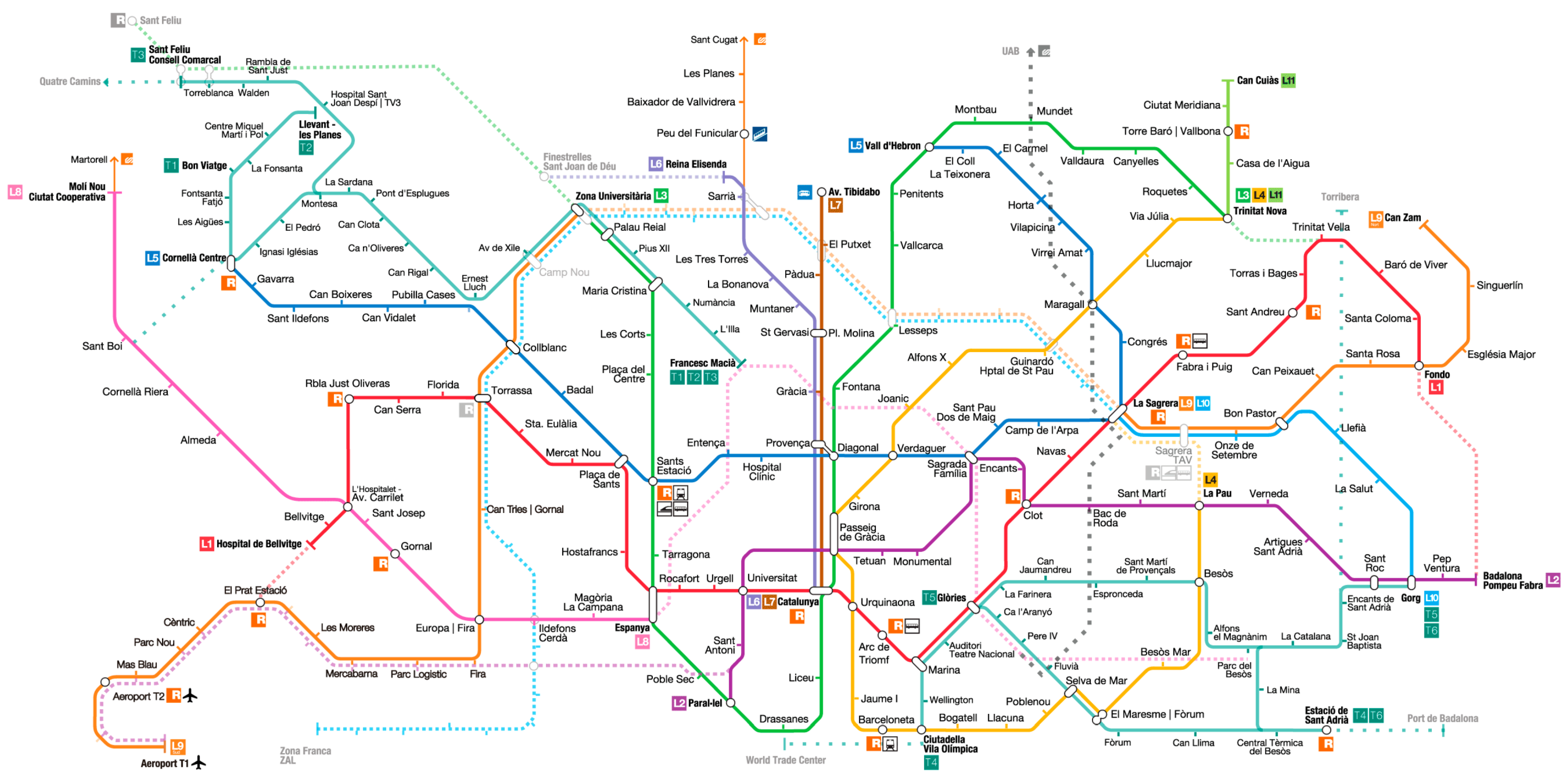
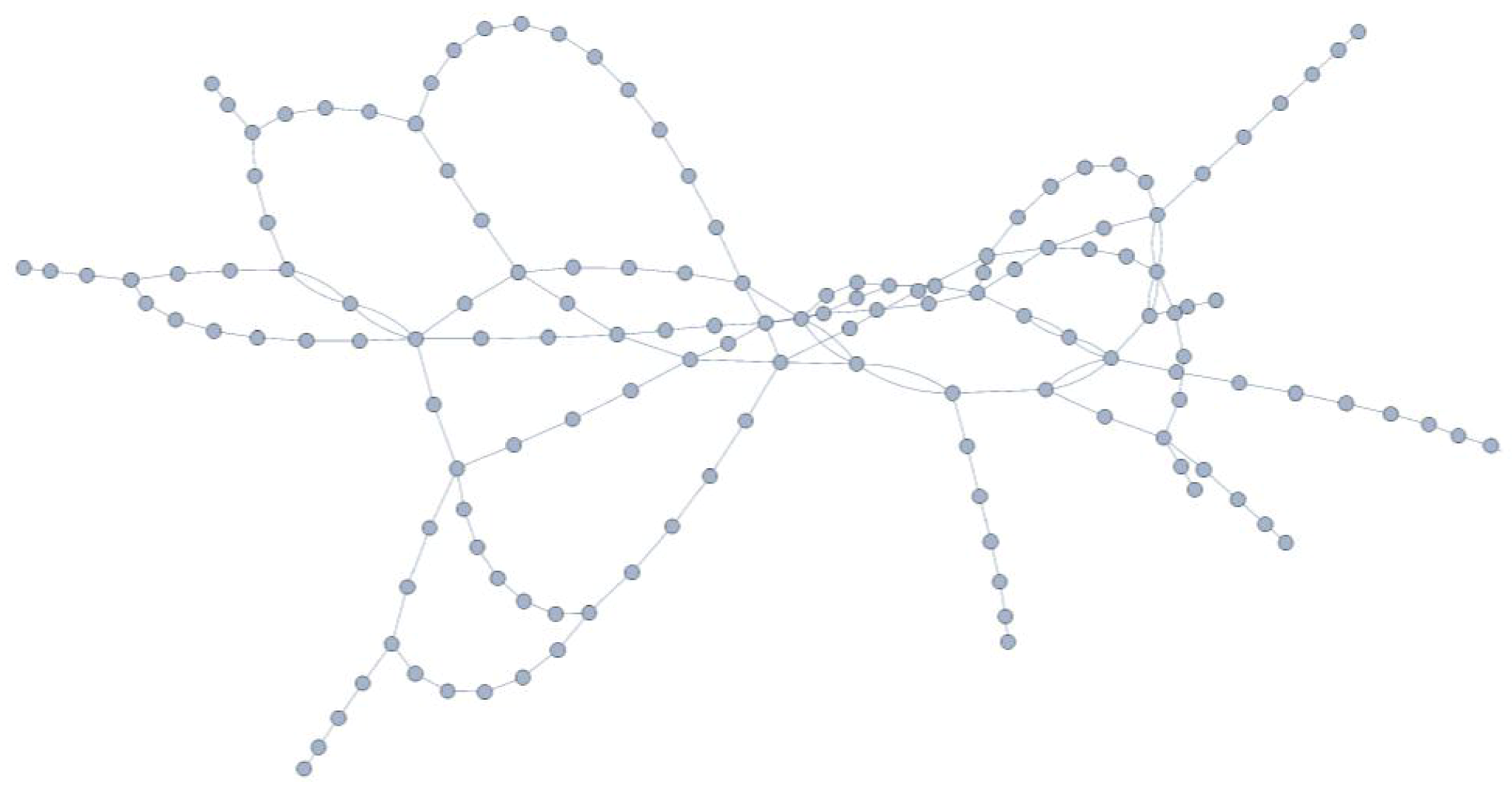
Two main goals are addressed in this work: (1) study the structural and robustness characteristics of Barcelona subway network; and (2) identify ridership patterns at its stations. In the first case, the basic techniques of Complex Network Analysis are used (centrality measures, structural indices, robustness coefficients, etc.), whereas, in the second case, a hierarchical cluster analysis is performed to group stations according to their boarding patterns. Barcelona’s metro is Spain’s second largest city subway system: there are a total of 13 lines and 151 stations in the network. Its length is 119 km, and during 2018 more than 400 million people used it.

In recent years, the complex network approach has been used to analyze the subway rail networks of several cities around the world. Since 2002, when Latora and Marchiori studied the topological properties of the Boston subway [2], many other works have appeared. Lu and Shi found that the public transportation network in China had scale-free and small world characteristics [3]. Zhang et al. studied the topological characteristics of some subway networks around the world and investigated network failures to discuss the vulnerability of these subway networks [4]. Liu and Song [5] studied the topology of Guangzhou subway network using L-space method, and the value and distribution of the network’s degree, clustering coefficient and average shortest path length were computed and analyzed. Cats [6] conducted a longitudinal analysis of the topological evolution of a multimodal rail network by investigating the dynamics of its topology for the case of Stockholm during 1950–2025.

The robustness of subway networks has also been discussed by many other researches. For example, Derrible and Kennedy studied the complexity and robustness of 33 metro networks [7]. Using network science and graph theory, ten theoretical and four numerical robustness metrics and their performance in quantifying the robustness of metro networks under random failures or targeted attacks were investigated by Wang et al. [8]. Zhang et al. [9] investigated the connectivity, robustness and reliability of the Shanghai subway network of China. Forero-Ortiz et al. [10] gave insights for stakeholders and policymakers to enhance urban flood risk management, as a reasonable approach to tackle this issue for Metro systems worldwide. De Bona et al. [11] proposed a novel methodology called Reduced Model as a simple method of network reduction that preserves the network skeleton (backbone structure) by properly removing 2-degree nodes of weighted and unweighted network representations. In [12], a new perspective for understanding vulnerability of metro networks is shown with the aims of improving operation reliability and stability of the network, designing emergency strategies to protect the network, etc.

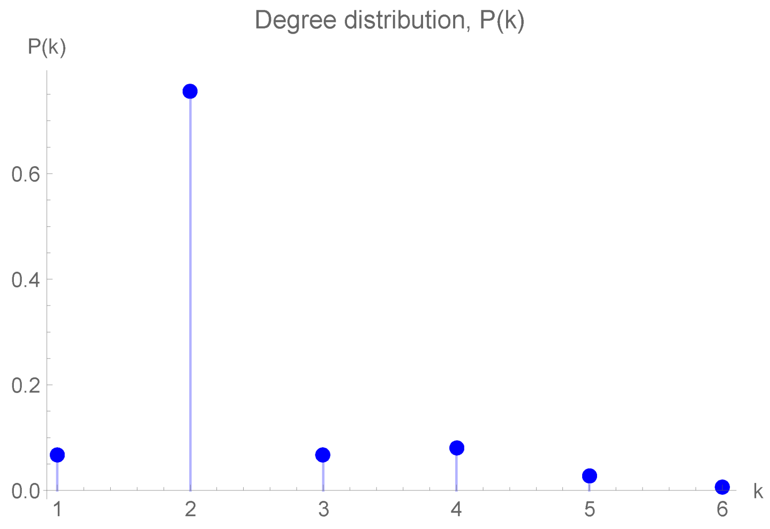
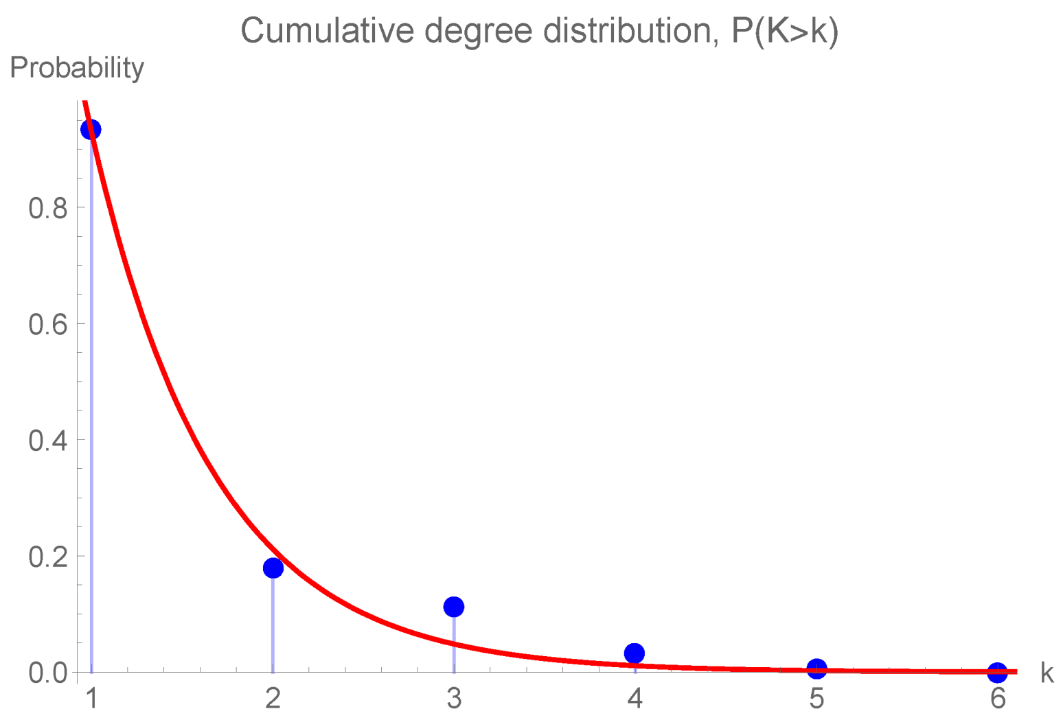
In this work, the topological characteristics of the metro network are investigated considering the complex network approach. Specifically a brief analysis of the Barcelona subway network is provided from the computation of the most important centrality measures: (i) degree centrality $C_D$; (ii) average degree $E\left[D\right]$; (iii) degree distribution $p\left(k\right)$; (iv) average path length L; (v) closeness centrality $C_{CL}$; and (vi) betweenness centrality $C_B$. In addition, to assess the robustness of the subway network, eight theoretical robustness metrics are investigated: (i) normalized robustness indicator ${\overline{r}}^T$; (ii) effective graph conductance $C_G$; (iii) average efficiency $E\left[\frac{1}{H}\right]$; (iv) clustering coefficient $C_{CG}$; (v) normalized algebraic connectivity ${\overline{\mu }}_{N-1}$; (vi) average degree $E\left[D\right]$, (vii) normalized natural connectivity $\overline{\lambda }$; and (viii) degree diversity $\kappa$.

Most public transit networks use automated fare collection (AFC) systems. The interest in this kind of technology is because it is perceived as a secure method of user validation and fare payment. Moreover, it improves the quality of the data, gives transit a more modern look and provides new opportunities for innovative and flexible fare structuring [13]. While the main purpose of AFC systems is to collect revenue, they also produce very large quantities of very detailed data of on-board transactions. These data are very useful to transit planners, from the day-to-day operation of the transit system to the strategic long-term planning of the network [14].

AFC systems are classified into two types according to the fare charge mode of transit: flat-rate fare systems and distance-based fare systems. In flat-rate fare systems, only entry swipes are registered, while, in distance-based fare systems, entry and exit swipes are registered. Barcelona metro uses a flat-rate fare system, therefore only metro boarding is available in this study. This has the inconvenience of not knowing where the passenger’s journey ends, e.g., the trip’s purpose. The destination of the trip helps understand peak hours. For instance, most of the work and education trips start in the morning peak from home and return back to home in the evening peak. While not within the scope of this paper, the destination estimation of public transport is one of the major concerns for the implementation of smart card data and there exist several approaches (see, e.g., [15,16,17,18]).

Every day, depending on the size of the network, millions of transactions are registered by the AFC systems, which can be used to analyze human mobility. It has been determined that human trajectories and trips generated with human mobility show a high degree of temporal and spatial regularity [19]. Passenger flow of the urban subway varies according to time and space, including working days, holidays, seasons, residential areas, business centers, workplaces and other factors such as weather, as well as other forms of transportation that connect to the subway network. In this regard, several methods have been developed in the literature for this type of analysis, most using clustering approaches [20].

Two viewpoints can be considered when a cluster analysis using smart card data is performed. The first one clusters stations based on the temporal-spatial distribution characteristics of subway ridership. The second one identifies groups of passengers that have similar boarding times aggregated into weekly profiles [21].

From the first point of view, Chen et al. [22] studied the diurnal pattern of subway ridership in New York City using the k-means algorithm. Wang et al. [23] analyzed eight metro stations in the central area of Hong Kong using the hierarchical cluster analysis. The k-means algorithm was also employed by Kim et al. [24] to identify the daily travel patterns at subway stations of Seoul Capital Area. Ding et al. [25] applied gradient boosting decision trees to investigate the non-linear effects of built environment variables on station boarding in the Washington metropolitan area. Langlois et al. [26] proposed a longitudinal representation of user’s multi-week activity and identified 11 travel patterns from London’s public transport network.

The study and analysis of different characteristics of subway networks have been tackled by means of other different paradigms. For example, risk analysis has been addressed in some recent works (see, e.g., [10,27,28,29]), the GIS-based technologies improves the analysis performed using mathematical methods [30], modern statistical and mathematical techniques can be also applied [31,32,33,34], the study of bus–metro transfers is considered in [35,36], etc. Moreover, techniques based on the Artificial Intelligence paradigm have also been used to study different aspects of subway networks (see, e.g., [37,38,39]).

The rest of the paper is organized as follows. Section 2 describes the data used in the study. Section 3 is devoted to presenting the methodology used for the analysis of travel patterns. Finally, the results obtained and the discussion are presented in Section 4 and the conclusions in Section 5.

2. Structural and Transit Data of Barcelona Subway Network

2.1. Study Area

Barcelona is considered a significant success in urban development across Europe. As the second largest city of Spain, it has been growing and transforming itself to be a knowledge-intensive city and, more importantly, a pioneer in being a smart city [40]. In addition, it has been one of the Spanish cities with the most confirmed cases of coronavirus. This is why it is an excellent case to explore.

Barcelona has an area of 102 km${}^2$ and a resident population of more than 1.62 million. The city has a diverse public transport system composed of metro, urban and intercity buses, commuter trains, tramway, funicular cable tramway and taxis.

The Barcelona Metro is a metropolitan railway network that gives service to Barcelona and the municipalities of its metropolitan area: Badalona, Cornellà de Llobregat, L’Hospitalet de Llobregat, Montcada i Reixac, El Prat de Llobregat, Sant Adrià de Besòs, Sant Boi de Llobregat and Santa Coloma de Gramanet. It comprises 13 lines with a length of 119 km (see Figure 1):

• L1: Hospital de Bellvitge–Fondo
• L2: Paral-lel–Badalona Centre
• L3: Zona Universitària–Trinitat Nova
• L4: La Pau–Trinitat Nova
• L5: Cornellà Centre–Vall d’Hebron
• L6: Plaça Catalunya–Reina Elisenda
• L7: Plaça Catalunya–Avinguda Tibidabo
• L8: Plaça Espanya -Molí Nou Ciutat Cooperativa
• L9 Nord: La Sagrera–Can Zam
• L9 Sud: Aeroport T1–Zona Universitària
• L10 Nord: La Sagrera–Gorg
• L10 Sud: Foc–Collblanc
• L11: Trinitat Nova–Can Cuiàs

2.2. Transit Data

The data used in this research correspond to the ridership (number of entries) in each station from 5 March 2018 to 11 March 2018. The reason this week was selected is because it is a week without public holidays or summer or winter holidays, and, therefore, it can reflect the general station ridership characteristics under normal circumstances. There was no extreme weather associated with that week either (e.g., heavy storms or very hot temperatures).

A statistical analysis of daily transit data was performed to analyze hourly inbound ridership of the 151 stations of Barcelona subway. The Barcelona metro operates from Sunday to Thursday from 5:00 to 24:00. On Fridays, the metro schedule is extended until 2:00, while on Saturdays it offers continuous service for 24 h. Thus, there are 140 variables for each station.

There are some aspects that need to be taken into account when addressing the analysis. First, it is important to notice there are two time-related patterns: the inbound ridership patterns on weekdays and at weekends. While they are both highly correlated on their own, the correlation between the ridership on weekdays and on the weekend is relatively low (see Figure 2). Second, from the analysis of the inbound ridership, it can be deduced that the highest peak hour during weekday mornings is between 7:00 and 8:00. During the evening rush hour, the highest peak hours are between 14:00 and 15:00 and between 18:00 and 19:00. Meanwhile, the rush hours during the weekend are from 13:00 to 14:00 and from 18:00 to 19:00 (see Figure 3). Figure 4, where the total number of entries at each hour is added up for all the days in the selected week for 35 randomly selected stations, illustrates how the different rush hours change depending on the station, and that both the time and the number of validations that represent a peak for a station vary. In addition, the total number of passengers significantly differs from one station to another. For instance, taking the daily ridership of 5 March, Diagonal station has a total of 54,636 passengers, while, at Casa de l’agua, there were only 207 boardings that day. These are the stations with the maximum and minimum total number of boardings and illustrate the huge difference there can be. Finally, as shown in Figure 5, the distribution of passenger flow decreases significantly on Saturdays and Sundays, which is why it was decided to focus on the data from Monday to Friday.

3. Methodology

3.1. Complex Network Analysis

In this study, the L-space representation of the network is considered. Hence, the stations of the subway network are represented by nodes of a graph and the tracks connecting two stations are represented by edges of the graph. Therefore, the subway network is represented by a undirected graph $G=\left(V,E\right)$ where $V=\{v_1,v_2,\dots ,v_N\}$ is the set of nodes, and $E=\{e_{ij}=\left(v_i,v_j\right),v_i,v_j\in V\}$ is the set of edges, where $\left|E\right|=M$.

The adjacency matrix of G, $A_G={\left(a_{ij}\right)}_{1\le i,j,\le N}$, is a $N\times N$ symmetric matrix such that the coefficient $a_{ij}$ takes the value 1 or 0 depending on whether or not there is a link between nodes $v_i$ and $v_j$. The degree of a node $v_i$ is the number of adjacent nodes to $v_i$ and can be computed as follows: $d_i={\sum }_{j=1}^N{a}_{ij}$.

The Laplacian matrix $Q_G=\Delta -A_G$ is an $N\times N$ matrix, where $\Delta =\mathrm{diag}\left(d_1,\dots ,d_N\right)$ is the $N\times N$ diagonal degree matrix. The eigenvalues of $Q_G$ play a very important role in robustness analysis; they are non-negative and can be ordered as $0={\mu }_N\le {\mu }_{N-1}\le \dots \le {\mu }_1$.

3.1.1. Centrality Measures

The analysis of a complex network is performed through the computation and analysis of several structural coefficients of the network topology. Specifically, the most important are the following [41]: degree centrality, average degree, degree distribution, average path length, closeness centrality and betweenness centrality.

The degree centralityof $v_i$ is the average number of incident edges to $v_i$:

$$C_D\left(v_i\right)=\frac{d_i}{N},$$

(1)

and the normalized average degree of the network G is given by:

$$\overline{E}\left[D\right]=\frac{{\displaystyle \sum _{i=1}^N}{d}_i}{N\left(N-1\right)}.$$

(2)

Moreover, the degree distribution of the network, $P\left(k\right)$, is the probability distribution of degrees over the whole network.

The shortest path length or distance between two nodes $v_i,v_j\in V$ is denoted by $d\left(v_i,v_j\right)$ and is defined as the minimum number of links necessary to go from node $v_i$ to node $v_j$. The average path length of the network is defined as the average distance between two nodes:

$$L=\frac{2}{N\left(N-1\right)}\sum _{1\le i<j\le N}d\left(v_i,v_j\right).$$

(3)

The diameter D of G is the greatest distance between any pair of nodes:

$$D=max\{d\left(v_i,v_j\right),v_i,v_j\in V\}.$$

(4)

The closeness centrality of the node $v_i$ measures the mean distance from $v_i$ to the rest of the nodes of the network:

$$C_{CL}\left(v_i\right)=\frac{1}{{\displaystyle \sum _{i\ne j}}d\left(v_i,v_j\right)}.$$

(5)

The greater is the value of closeness centrality, the smaller is the length of the shortest paths to all other nodes.

Finally, the betweenness centrality of the node $v_i\in V$ measures the number of shortest paths between two nodes that run through node $v_i$. Mathematically it is defined as follows:

$$C_B\left(v_i\right)=\frac{2}{\left(N-1\right)\left(N-2\right)}\sum _{r\ne s\ne i}\frac{{\ell }_{rs}\left(v_i\right)}{{\ell }_{rs}},$$

(6)

where ${\ell }_{rs}$ is the total number of shortest paths from $v_r$ to $v_s$ and ${\ell }_{rs}\left(v_i\right)$ is the the number of shortest paths between $v_r$ and $v_s$ that pass through $v_i$. In networks, the greater is the number of paths that pass through a node, the greater is the importance of this node and more central it is.

3.1.2. Theoretical Robustness Metrics

Robustness can be defined as the network’s ability to survive random failures or deliberate attacks consisting of the elimination of nodes and/or edges [42]. In this sense, several robustness measures have been proposed to quantitatively determine this characteristic. The most important ones are described in what follows:

The normalized robustness indicator ${\overline{r}}^T$ measures the ratio between the number of alternative paths in the network topology and the total number of stations [8]:

$${\overline{r}}^T=\frac{ln(M-N+2)}{ln\left(\frac{N(N-1)}{2}-N+2\right)}.$$

(7)

Note that ${\overline{r}}^T$ is higher in the case there are alternative routes to reach a destination and it is smaller in large systems.

The effective graph resistance $R_G$ estimates the robustness of a network from the number of parallel paths (i.e., redundancy) and the length of each path between each pair of nodes. The effective graph resistance is calculated in terms of the eigenvalues of the Laplacian matrix as follows:

$$R_G=N\sum _{i=1}^{N-1}\frac{1}{{\mu }_i}.$$

(8)

In this work, the normalized version of the the effective graph resistance, called effective graph conductance [43], is used:

$$C_G=\frac{N-1}{R_G}.$$

(9)

Note that $0\le C_G\le 1$ and a larger $C_G$ indicates a higher level of robustness.

The average efficiency$E\left[\frac{1}{H}\right]$ is defined as follows [44]:

$$E[\frac{1}{H}]=\frac{2}{N(N-1)}\sum _{i,j=1,i\ne j}^N\frac{1}{d(v_i,v_j)}.$$

(10)

Note that the greater is the value of the average efficiency, the greater is the robustness of the network (recall that the global efficiency of the complete network is 1).

The clustering coefficient is used to assess how the neighbors of a node are connected with one another [41]. For node $v_i$, it is mathematically defined as follows:

$$C_C\left(v_i\right)=\frac{2E_i}{d_i\left(d_i-1\right)},$$

(11)

where $E_i$ is the number of edges linked to the neighbors of node $v_i$. The clustering coefficient shows the fault tolerance characteristic: in a subway network, when one station is out of function, the traffic will not be affected if the neighboring stations are connected. Thus, a larger value of $C_C$ implies a better tolerance to fault in a local scale. The average clustering coefficient is the average of all the individual clustering coefficients:

$$C_{CG}=\frac{1}{N}\sum _{i=1}^{N}CC\left(v_i\right).$$

(12)

The algebraic connectivity ${\mu }_{N-1}$ is the second smallest eigenvalue of the Laplacian matrix $A_G$. It has been shown that the larger ${\mu }_{N-1}$ is, the higher the robustness of a network is [43]. The normalized algebraic connectivity is obtained dividing by the total number of nodes: ${\overline{\mu }}_{N-1}=\frac{{\mu }_{N-1}}{N}$.

The normalized natural connectivity $\overline{\lambda }$ is defined as:

$$\overline{\lambda }=\frac{ln[\frac{1}{N}{\displaystyle \sum _{i=1}^N}{e}^{{\lambda }_i}]}{N-lnN},$$

(13)

where ${\lambda }_i$ is the ith eigenvalue of the adjacency matrix $A_G$. It measures the redundancy in terms of alternative paths and is considered as a measure of structural robustness [45].

Finally, the degree diversity $\kappa$ is defined as:

$$\kappa =\frac{{\displaystyle \sum _{i=1}^N}{d}_i^2}{{\displaystyle \sum _{i=1}^N}{d}_i}.$$

(14)

The greater $\kappa$ is, the more nodes must be removed from the network to disintegrate it [46]. In this work, we take the inverse of the degree diversity $\overline{\kappa }=\frac{1}{\kappa }$ in order to scale the value in the interval $[0, 1]$.

3.2. Normalization and Dimensionality Reduction

Given the large differences in the number of passengers from station to station, the entries are normalized. The normalization consists in using the ratio of hourly passengers to the total number of passengers that day at each station, instead of the total amount of passengers per hour [24].

On the other hand, the number of variables used to classify the stations is large and they are also highly correlated; therefore, it was decided to perform a Principal Component Analysis (PCA). PCA is a technique for reducing the dimensionality of large datasets, increasing interpretability and minimizing information loss [47]. PCA is defined as an orthogonal linear transformation which transforms the data into a new system of coordinates such that the first coordinate (called the first principal component) represents the largest variance, the second coordinate the second greatest, etc. PCA can be thought of as fitting an n-dimensional ellipsoid to the data, where each axis of it represents a principal component. If an axis of the ellipse is small, then the variance along that axis is also small. To find the axes of the ellipse, first the mean of each variable from the dataset must be subtracted to center the data around the origin. Then, the covariance matrix of the data is computed. The covariance between two data is calculated as:

$${\sigma }_{jk}=\frac{1}{n-1}\sum _{i=1}^n(x_{ij}-{\overline{x}}_j)(x_{ik}-{\overline{x}}_k)$$

(15)

The principal components are calculated from the eigen-vectors and eigenvalues of this matrix. The eigenvectors represent the directions, whereas the eigenvalues are the numbers representing how much variance there is in the data in each particular direction. The eigenvector with the highest eigenvalue is taken as the first principal component. More details can be found in the work of Dunteman [48].

3.3. Clustering Analysis

Cluster analysis is an exploratory technique which is used to classify objects into groups, known as clusters, in such way that observations belonging to a cluster are more similar to each other than observations assigned to different clusters. Nevertheless, clustering is rather a subjective statistical analysis and there are several possible algorithms that may be used. The decision of which technique to apply should be made depending on the kind of data or the type of problem to be solved. The k-means algorithm is known to be computationally fast and has the ability to handle large datasets. However, one needs to know the number of clusters in advance, it is sensitive to outliers and different initial centroids produce different results [49]. Hierarchical clustering is one of the most popular clustering techniques. Although it may be computationally slower when the dataset size increases and clusters depend on the distance metric used, the authors consider that the result of a hierarchical clustering is a structure that is more informative and interpretable than the unstructured set of flat clusters returned by k-means. Hence, it is easier to determine the optimal number of clusters by looking at the dendrogram of a hierarchical clustering than trying to predict this optimal number in advance in case of k-means. For these reasons, the agglomerative hierarchical clustering technique is used [50]. The basic algorithm consists of the following steps:

• Initially, each observation is considered as a single-element cluster.
• An iterative process is then initiated in which the two clusters that are the most similar are combined into a new bigger cluster. This is done by computing the dissimilarities between every pair of observations. This procedure is iterated until all points are members of one single big cluster.
• Finally, one needs to determine where to cut the hierarchical tree into clusters. This creates a partition of the data.

The distance between clusters can be calculated using different methods [51,52]. In this study, the Ward method was used, which has been very widely used since its first description by Ward Jr [53], it and has outperformed other methods in several comparison studies [54,55]. The Ward method is the only one among the agglomerative clustering methods that is based on a classical sum-of-squares criterion, producing groups that minimize within-group dispersion at each binary [56]. In the Ward method, the distance between two clusters, A and B, is how much the sum of squares will increase once they are merged:

$$\begin{array}{cc}\hfill \Delta (A,B) =& \sum _{i\in A\cup B}\parallel {\overrightarrow{x}}_i-{\overrightarrow{m}}_{A\cup B}{\parallel }^2-\sum _{i\in A}\parallel {\overrightarrow{x}}_i-{\overrightarrow{m}}_A{\parallel }^2-\sum _{i\in B}{\parallel {\overrightarrow{x}}_i-{\overrightarrow{m}}_B\parallel }^2\hfill \\ \hfill =& \frac{n_A{n}_B}{n_A+n_B}{\parallel {\overrightarrow{m}}_A-{\overrightarrow{m}}_B\parallel }^2,\hfill \end{array}$$

(16)

where ${\overrightarrow{m}}_j$ is the center of cluster j and $n_j$ is the number of points in it. $\Delta$ is called the merging cost of combining the clusters A and B. In this method, in each step, the variability within clusters is minimized.

In addition, the agglomerative coefficient (AC), measuring the clustering structure of the dataset, is calculated [57]. For each observation i, let $m\left(i\right)$ represent its dissimilarity to the first cluster it is merged with, divided by the dissimilarity of the merger in the final step of the algorithm. The AC is the average of all $1-m\left(i\right)$. Generally speaking, the AC describes the strength of the clustering structure that has been obtained by group average linkage. However, the AC tends to become larger when n increases, so it should not be used to compare datasets of very different sizes. The coefficient takes values from 0 to 1, and it is actually the mean of the normalized lengths at which the clusters are formed. A coefficient close to 1 points to a pretty reasonable cluster structure in the data.

4. Mathematical and Statistical Analysis

4.1. Structural Network Analysis

As previously mentioned, the topology of Barcelona subway network is established using the L-space method, where each station stands for a node of the graph and the edges are defined by means of the direct connections by rail ways between the stations. The number of nodes is $N=151$ and the number of edges is $M=177$ and therefore the density of the subway network is $d\approx 0.0157$. In Figure 6, the graph corresponding to Barcelona subway network using Mathematica is shown (note that the exact placing and positioning of the stations is not taken into account).

4.1.1. Basic Structural Characteristics

In this subsection, the most usual coefficients and centrality measures, introduced in Section 3.1.1, are computed and associated to the Barcelona subway network.

As shown in

Table 1. The five stations with the highest degree.

Station	Subway Lines	Degree
Passeig de Gràcia	2, 3, 4	6
Diagonal	3, 5	5
Espanya	1, 3	5
Catalunya	1, 3	5
La Sagrera	1, 5, 9N, 10N,	5

the five stations with the highest degree are “Passeig de Gràcia” with degree 6 and “Diagonal”, “Espanya”, “Catalunya” and “La Sagrera” with degree 5. Note that the first four stations belong to Line 3; in addition, three of the top five are on Line 1.

The average degree of the network is $E\left[D\right]\approx 2.2649$ and the degree distribution $p\left(k\right)$ is shown in Figure 7, while the cumulative degree distribution is illustrated in Figure 8. A simple calculus shows that the fitting function of the cumulative degree distribution is $h\left(x\right)=4.0834e^{-1.4796x}$.

The maximum travel distance of the network is no more than 31 stops (diameter), while the average shortest path is 11.0032 stops.

Table 2. The five stations with the highest closeness centrality.

Station	Subway Lines	Closeness Centrality
Diagonal	3, 5	0.1424
Verdaguer	4, 5	0.1372
Hospital Clìnic	5	0.1362
Passeig de Gràcia	2, 3, 4	0.1358
Provença	3, 5, 6, 7	0.1323

shows the results obtained from the computation of the closeness centrality. The station with the highest closeness centrality is “Diagonal” with $C_{CL}\approx 0.1424$, and the next four stations (“Verdaguer”, “Hospital Clìnic”, “Passeig de Gràcia” and “Provença”) have similar closeness centrality. In this case, the most centrality subway line is Line 5 and, to a lesser extent, Line 3.

Finally, the results obtained when the betweenness centrality was computed are displayed in

Table 3. The five stations with the highest betweenness centrality.

Station	Subway Lines	Betweenness Centrality
Diagonal	3, 5	0.4298
Verdaguer	4, 5	0.3333
Sants Estaciò	3, 5	0.2610
Hospital Clìnic	5	0.2593
Entença	5	0.2553

. It is important to note that all the stations with the highest coefficient belong to Line 5.

From these results, it can be seen that some specific stations play a central role in the structural definition of the network. For example, “Diagonal” and “Verdaguer” are very important structural pieces of the subway network since they have the highest values of closeness and betweenness centralities. In addition the most central lines are Lines 5, 3 and 1.

4.1.2. Network Robustness

Failures of subway networks can have enormous impact on our society, so the analysis of the robustness is very important when studying subway networks. The robustness of networks reflects the extent to which the networks can solve possible (intentional or unintentional) failures by offering alternative routes that overcome the attacked edges or nodes.

In this section, eight robustness metrics (introduced in Section 3.1.2 are computed for the Barcelona subway network and compared with those obtained for the Madrid subway network.

In

Table 4. Stations with non-zero clustering centrality.

Station	Subway Lines	Clustering Centrality
Catalunya	1, 3	0.2
Universitat	1, 2	0.1666
Urquinaona	1, 4	0.1666
Passeig de Gràcia	2, 3, 4	0.1333

, the stations with the highest clustering centrality are illustrated. The most central are “Catalunya” ($C_C=0.2$), “Universitat” and “Urquinaona” with $C_C\approx 0.1666$ and “Passeig de Gràcia” with $C_C\approx 0.1333$. As a consequence, they have better tolerance to fault in a local scale. The first three stations belong to Line 1, and Lines 2–4 have a couple of stations on this list. Moreover, the mean clustering coefficient is $0.0044$, which is significantly lower than that of other metro networks such as London ($C_C=0.0409$), Tokyo ($C_C=0.0285$) or Paris ($C_C=0.0163$) [58].

Table 5. Robustness metrics in Barcelona and Madrid subway networks.

Coefficients	Barcelona Subway	Madrid Subway
Nodes, N	151	243
Edges, M	177	280
Normalized robust indicator, ${\overline{r}}^T$	0.35747	0.35635
Efective graph conductance, $C_G$	0.00221	0.00086
Average efficiency, $E\left[\frac{1}{H}\right]$	0.13524	0.10533
Average clustering coefficient, $C_{CG}$	0.00441	0.00774
Normalized algebraic connectivity, ${\overline{\mu }}_{N-1}$	0.00006	0.00001
Normalized average degree, $\overline{E}\left[D\right]$	0.01562	0.00952
Normalized natural connectivity, $\overline{\lambda }$	0.00770	0.00441
Normalized degree diversity, $\overline{\kappa }$	0.35975	0.37135

shows the values of the eight robustness metrics computed using Equations (7)–(14) for the Barcelona subway network and the Madrid subway network [59].

According to the reduced robustness indicator ${\overline{r}}^T$, the Barcelona metro network is slightly more robust than the Madrid metro network, probably because there are more alternative paths between any pair of nodes.

According to the effective graph conductance $C_G$, the Barcelona subway network also has a slightly higher value than that of Madrid. Note that the effective graph conductance takes into account not only the number of alternative paths but also the length of each alternative path, hence effective graph conductance favors networks with the smallest length of the shortest paths.

In general, according to all the metrics except the clustering coefficient $C_{CG}$ and the normalized degree diversity $\overline{\kappa }$, Barcelona has a higher robustness level than Madrid.

4.2. Data Analysis Results

Principal component analysis was performed to study the data from the working days (Monday to Friday) of the selected week. The first three principal components are able to explain $66.32\%$ of the variability in the data ($\mathrm{PC}1=46.56\%$, $\mathrm{PC}2=12.88\%$ and $\mathrm{PC}3=6.89\%$). Figure 9 shows the total variability explained by each principal component.

In Figure 10, the top plot shows the contributions of 18 variables to the first three components. The six variables which most contribute to each component are chosen. In the bottom plot, the correlations of these 18 variables to each component are shown. The contribution is represented both by the color scale and the circle size, while, for the correlation, the direction of the correlation is represented by color and the circle size represents the strength of the relationship. The variables which contribute the most to the first component are those corresponding to 7 a.m., and they are strongly negatively correlated with it. Regarding the second component, the variables which contribute the most are the ones corresponding to 11 a.m. and noon. Finally, the variables contributing to the third component are the ones from 1 and 11 p.m. The second and third components have a positive correlation with the variables that contribute the most to them.

A hierarchical cluster analysis was performed over the coordinates from the first three principal components. The resulting AC is 0.9811, which indicates a pretty reasonable cluster structure in the data. The dendrogram in Figure 11 shows that two clustering solutions are possible. The four-cluster solution is chosen as it provides a more detailed segmentation of the stations.

Statistical properties of the four clusters are summarized in

Table 6. Statistical properties of the four clusters (weekdays).

Cluster	1	2	3	4
Size	49	41	35	4
Diameter	17.49	9.39	9.32	8.46
Average distance	7.55	4.15	3.58	5.42
Median distance	7.30	4.05	3.45	5.21
Separation	1.64	1.08	1.08	7.70
Average to other	12.76	9.32	11.79	19.93

. The diameters represent the maximum within cluster distances. The average and median distances are the within cluster average and median distances. Separation is the minimum distance of a point in the cluster to a point of another cluster and average to other is the average distance of a point in the cluster to the points of other clusters.

In

Table 7. Results of station classification.

Cluster	Stations	Number
Cluster 1	Aeroport T1, Aeroport T2, Arc de Triomf, Barceloneta, Bogatell, Casa de l’aigua, Catalunya, Ciutadella, Diagonal, Drassanes, El Maresme-Fórum, Entença, Espanya, Europa-Fira, Fontana, Girona, Gloriès, Guinardó, Hospital Cliníc, Hospital de Bellvitge, Hospital de Sant Pau, Hostafrancs, Jaume I, Joanic, Les Corts, Lesseps, Liceu, LLacuna, Maria Cristina, Marina, Monumental, Mundet, Palau Reial, Parallel, Passeig de Gràcia, Penitents, Poblenou, Rocafort, Sagrada Familia, Sant Antoni, Selva de Mar, Tetuan, Universitat, Urgell, Urquinaona, Vall d’Hebron, Verdaguer, Verneda, Zona Universitària	49
Cluster 2	Alfons X, Av. Carrilet, Bac de roda, Badal, Badalona - Pompeu Fabra, Baró de viver, Bellvitge, Bon pastor, Camp de l’arpa, Can tries - Gornal, Clot, Collblanc, Congrés, Cornellà Centre, El Coll - La Teixonera, Encants, Fabra I Puig, Horta, La Pau, Les Moreres, Llucmajor, Maragall, Mercat Nou, Montbau, Navas, Onze De Setembre, Parc Nou, Plaça De Sants, Plaça Del Centre, Poble Sec, Rbla. Just Oliveras, Sagrera, Sant Andreu, Sant Martí, Santa Eulàlia, Sants Estació, Tarragona, Torras I Bages, Torre Baró - Vallbona, Vallcarca, Virrei Amat	41
Cluster 3	Artigues - Sant Adrià, Besòs, Besòs Mar, Can Boixeres, Can Cuiós, Can Peixauet, Can Serra, Can Vidalet, Can Zam, Canyelles, Cèntric, Ciutat Meridiana, El Carmel, El Prat Estació, Església Major, Florida, Fondo, Gavarra, Gorg, La Salut, Llefià, Pep Ventura, Pubilla Cases, Roquetes, Sant Ildefons, Sant Roc, Santa Coloma, Santa Rosa, Singuerlín, Torrassa, Trinitat Nova, Trinitat Vella, Valldaura, Via Júlia, Vilapicina	35
Cluster 4	Fira, Mas Blau, Mercabarna, Parc Logístic	4

, the stations belonging to each cluster are listed. For a better understanding of the clusters, the different stations of each cluster are located in the Barcelona map, making use of a Voronoi diagram (based on Euclidean distance) to partition the city map. In Figure 12, each Voronoi cell representing a station is colored by cluster. It may be noted that stations from the same cluster are not necessarily close in space, but their behavior pattern is similar. This may be due to, e.g., the business activities taking place in the area or being residential neighborhoods.

In the case of Cluster 1, most of the stations are located in the district of L’Eixample, Ciutat Vella and Sant Martí, where some of the most popular beaches of Barcelona are located, as well as important monuments such as Casa Milà, popularly known as La Pedrera, the Cathedral, Park Güell and Casa Batlló. Moreover, this cluster includes the zoo, the Maritime Museum of Barcelona and the museum Poble Espanyol. The hospital stations Vall d’Hebron, Hospital Cliníc, Sant Pau and Hospital de Bellvitge are included in this cluster too, as well as those belonging to university campuses, such as Mundet, Palau Reial, Universitat and Zona Universitària. There are also two stations from the airport and some stations from the districts Les Corts, Sants, Montjuic and Gracia, all of them located in the city center. In Figure 13, passenger flow per hour is shown for some of the stations in Cluster 1. All of them have peak hours at 8 a.m., 2 p.m. and 7 p.m.

The stations in Cluster 2 are mainly around the central area of Barcelona, with some in the north and some in the south. These are traditional, residential, well-communicated neighborhoods, with many markets and shops. The stations in the north are from the districts Sant Andreu, Horta-Ginardó and Nou Barris. The stations in the south belong to L’Eixample and are the furthest from the city center together with the stations from Sant Andreu, one of the entrances to Barcelona with a large cultural and sports offer. The hours with the largest number of passengers in this cluster are 7 a.m., 8 a.m. and 6 p.m. The pattern of boarding per hour for some stations in this cluster is shown in Figure 14.

Cluster 3 contains mostly stations located outside of the city. There are two stations in El Prat de Llobregat and eight bordering the north side of L’Hospitalet de Llobregat. The rest are gathered in the north urban periphery of the city, linking to different small municipalities or towns, such as Badalona, Santa Coloma de Gramenet or Sant Adrià de Besòs. These belong to what is known as the metropolitan area of Barcelona, which is a geographical area that goes beyond the administrative area. Given the growth of the city of Barcelona, some of these municipalities are now essentially suburbs of Barcelona. Badalona is, however, the third largest city in Catalonia. Moreover, there are also stations in Ciutat Meridiana, which is the poorest neighborhood of the city. In Figure 15, the peak hours of the stations of this cluster can be seen. The hours with the highest number of boardings are 8 a.m., 2 p.m. and 6 p.m.

The stations that form Cluster 4 have the particular characteristics of the area they give access to: Fira is the entry to one of the largest and most modern fairgrounds of Europe; Mas Blau corresponds with the industrial park closest to Barcelona’s airport; Mercabarna is considered the most important central market in Europe, as it is a reference center in the Mediterranean Sea for the distribution of fresh products at the international level; and Parc Logístic serves the logistics park of the city’s Free economic zone. Overall, 2 p.m., 5 p.m. and 6 p.m. have the highest number of boardings. The peak hours of these stations are shown in Figure 16.

All the analysis here presented were performed with RStudio Team [60].

5. Conclusions

In Barcelona, as in any major urban area, many people use the public transport network, which is why it is necessary to have as much information as possible to forecast and plan the subway trip.

Moreover, in the bibliography studied, there are no previous studies that analyze not only the structural and robustness characteristics but also travel patterns of the Barcelona metro network.

In this study, a detailed analysis of Barcelona subway network was done using Complex Network Analysis. To achieve this goal, the most important centrality measures and coefficients were computed. In this sense, the important role of stations such as “Diagonal” and “Verdaguer” to control the flow of passengers was shown. It was also shown that the stations “Catalunya”, “Universitat”, “Urquinaona” and “Passeig de Gràcia” have high fault tolerance in a local scale. Moreover, L5 and L3 are the most central subway lines.

In addition, the robustness of the Barcelona subway network was investigated by analyzing several robustness metrics and compared with the robustness of the Madrid subway network. The results indicate that the Barcelona subway network is slightly more robust than the Madrid subway network according to most of the robustness metrics. A previous study [8] analyzed Barcelona subway robustness using ten theoretical robustness metrics, but only taking into account terminals and transfer stations. The results in the former study cannot be compared with ours since in our study all Barcelona subway stations are used.

The data collected at the entry of the metro stations in Barcelona provide a vast quantity of data with very valuable information about the ridership patterns in them. The set of real data was provided by the Barcelona Metropolitan Network, providing information on the number of entries per hour in each of the 151 stations. There are no data related to the passenger’s journey or personal data (age, sex, fare, etc.).

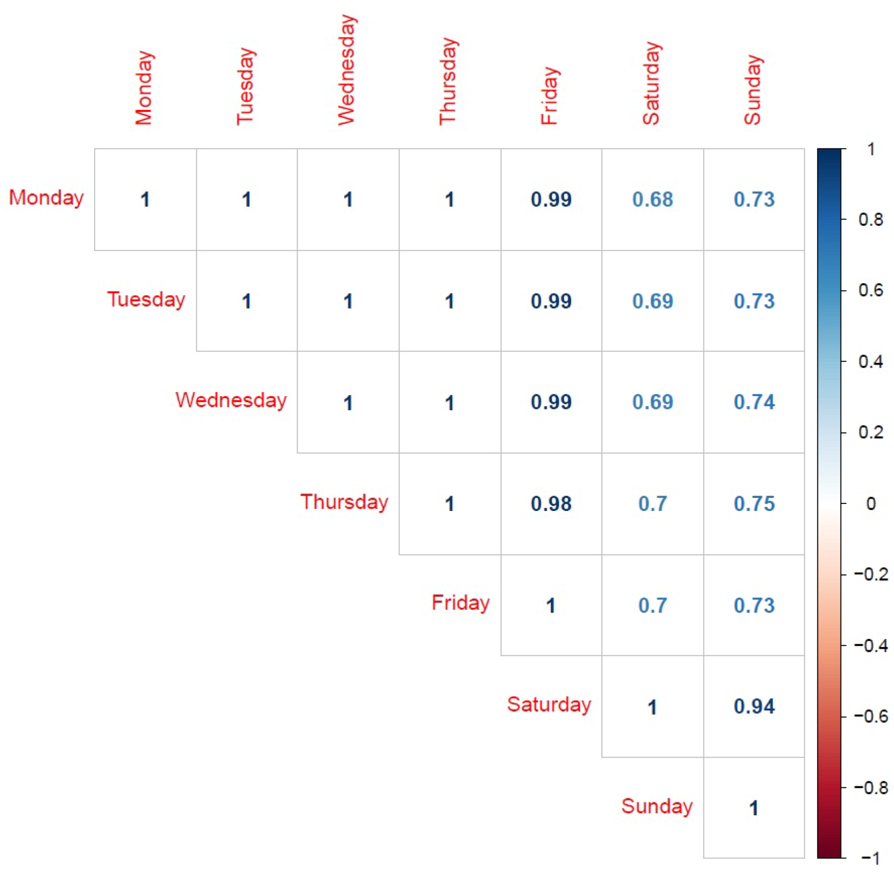
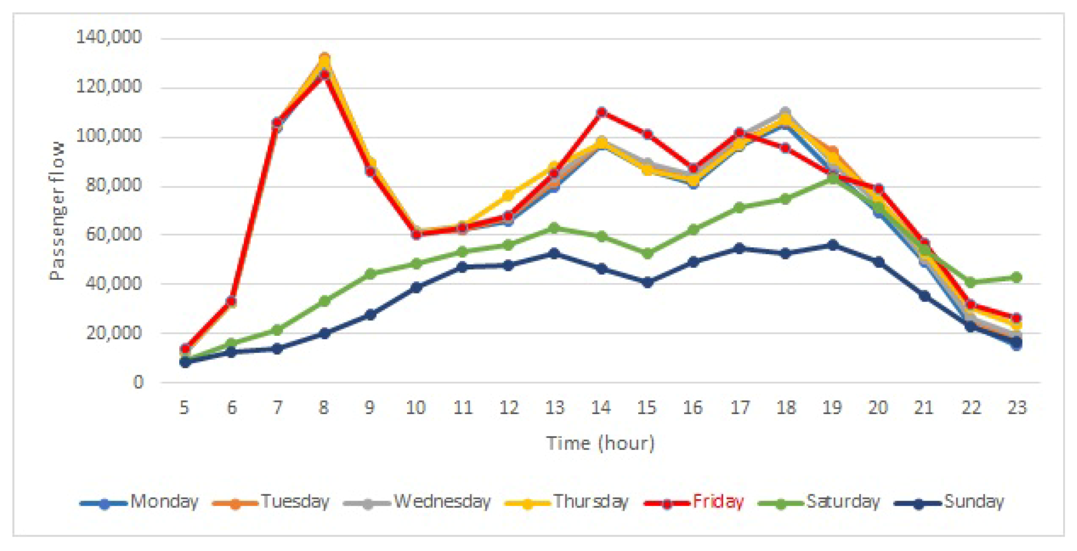
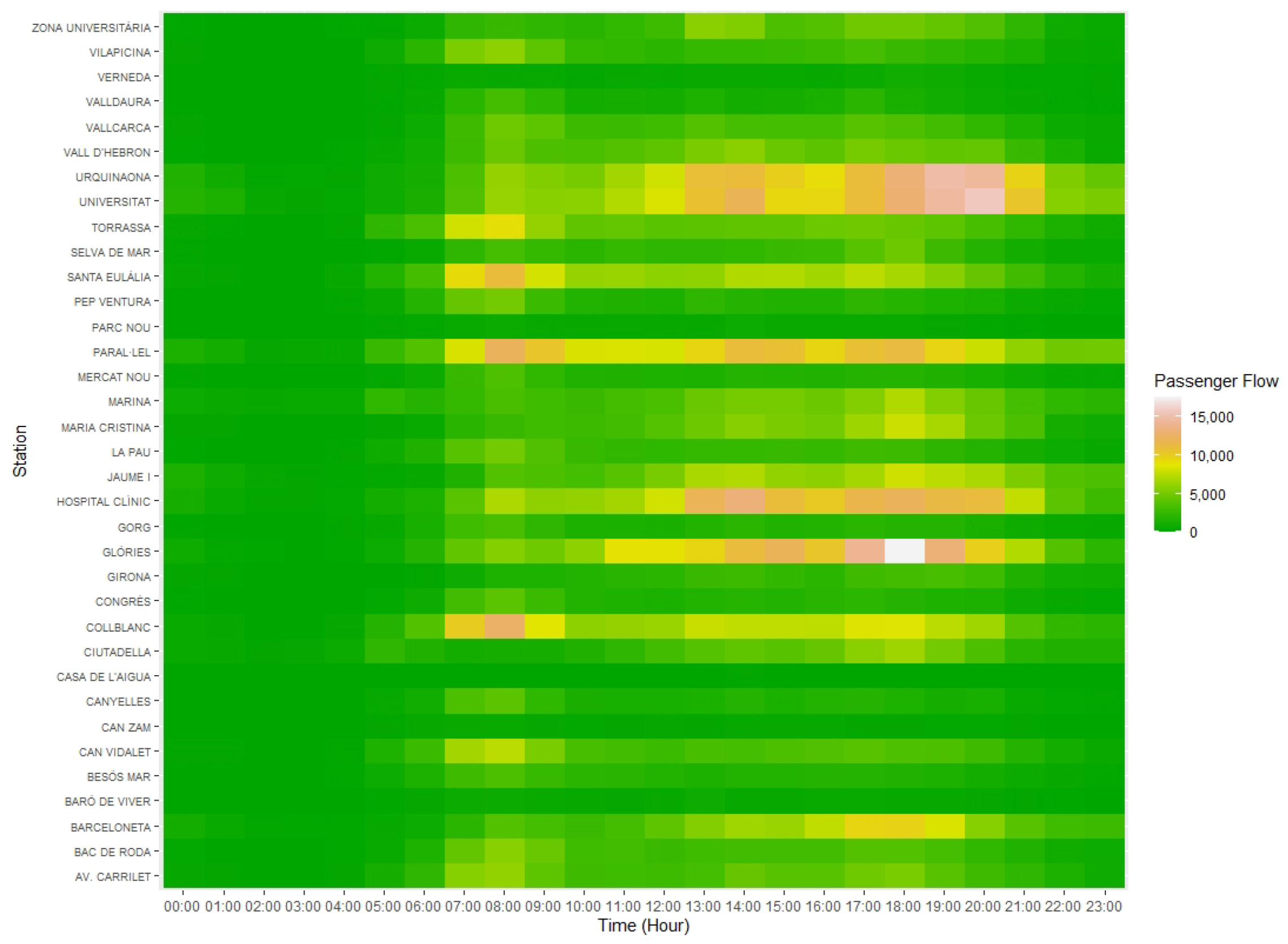
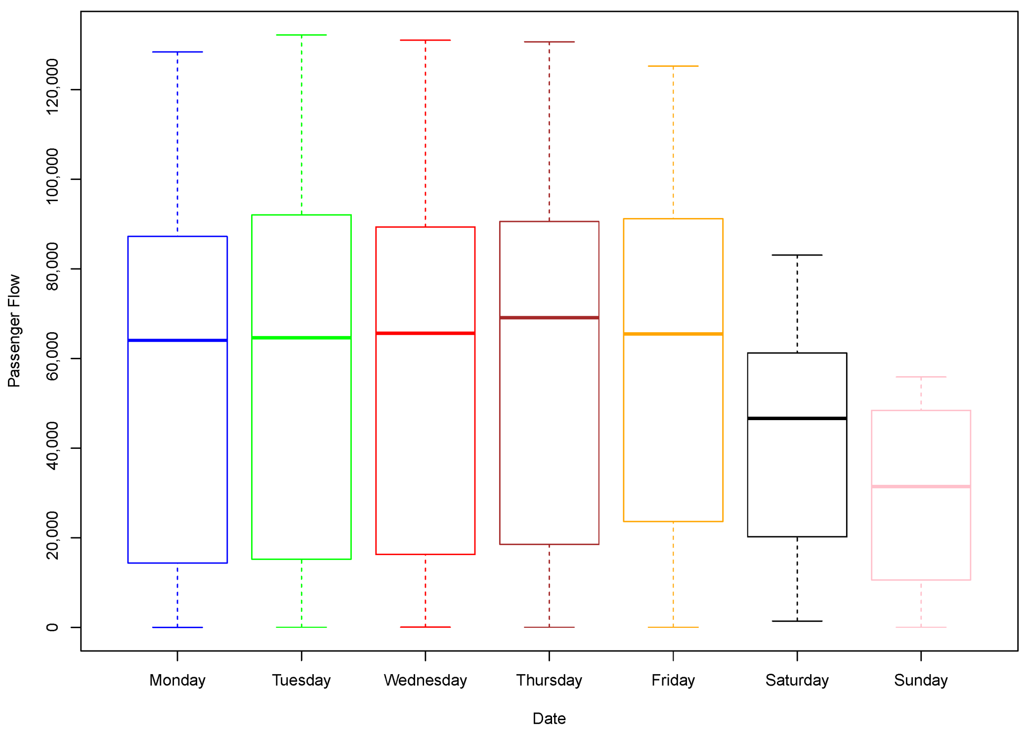
The statistical techniques used in this study allowed observing the following: in the first place, there are differences in behavior between working days, which are highly correlated with each other, and over the weekend, with which the correlation decreases. The hours with the highest number of passengers correspond mainly to the hours of entry and exit of work and school hours. However, these rush hours are not the same at all stations, nor are the number of passengers each have, reaching a difference of more than 54,000 daily entries between some stations. It is because of this reason that the data were normalized, using the proportion of passengers per hour with respect to the total number of entries in that particular day at each particular station.

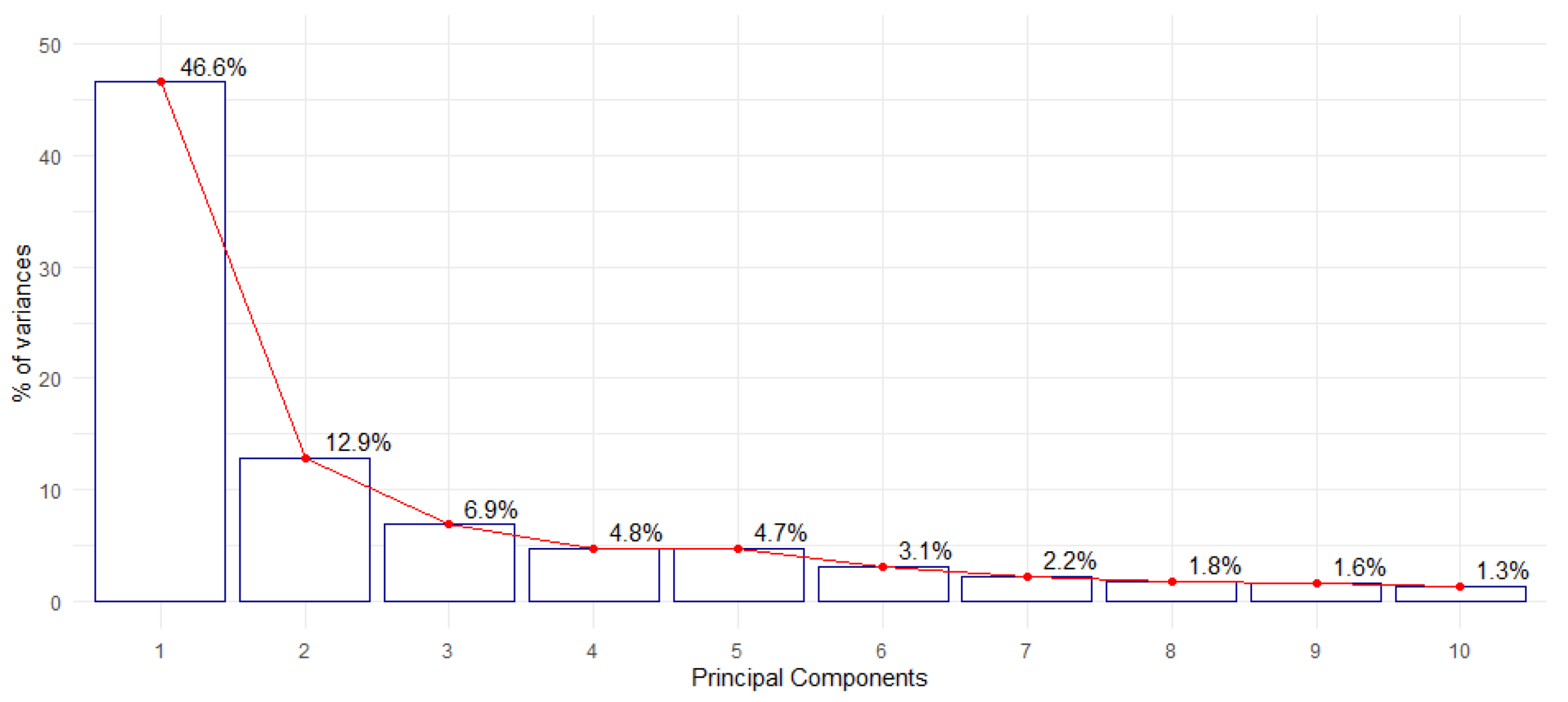
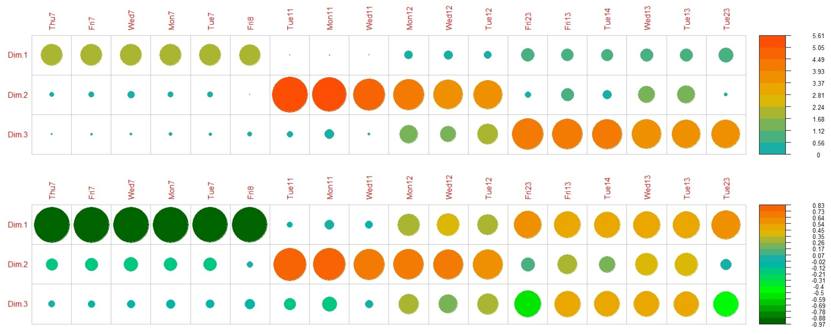
The principal component analysis performed reduced the dimensionality of the dataset. The first three principal components explain most of the variability in the data. Moreover, it was observed which hours have a higher effect in each of them.

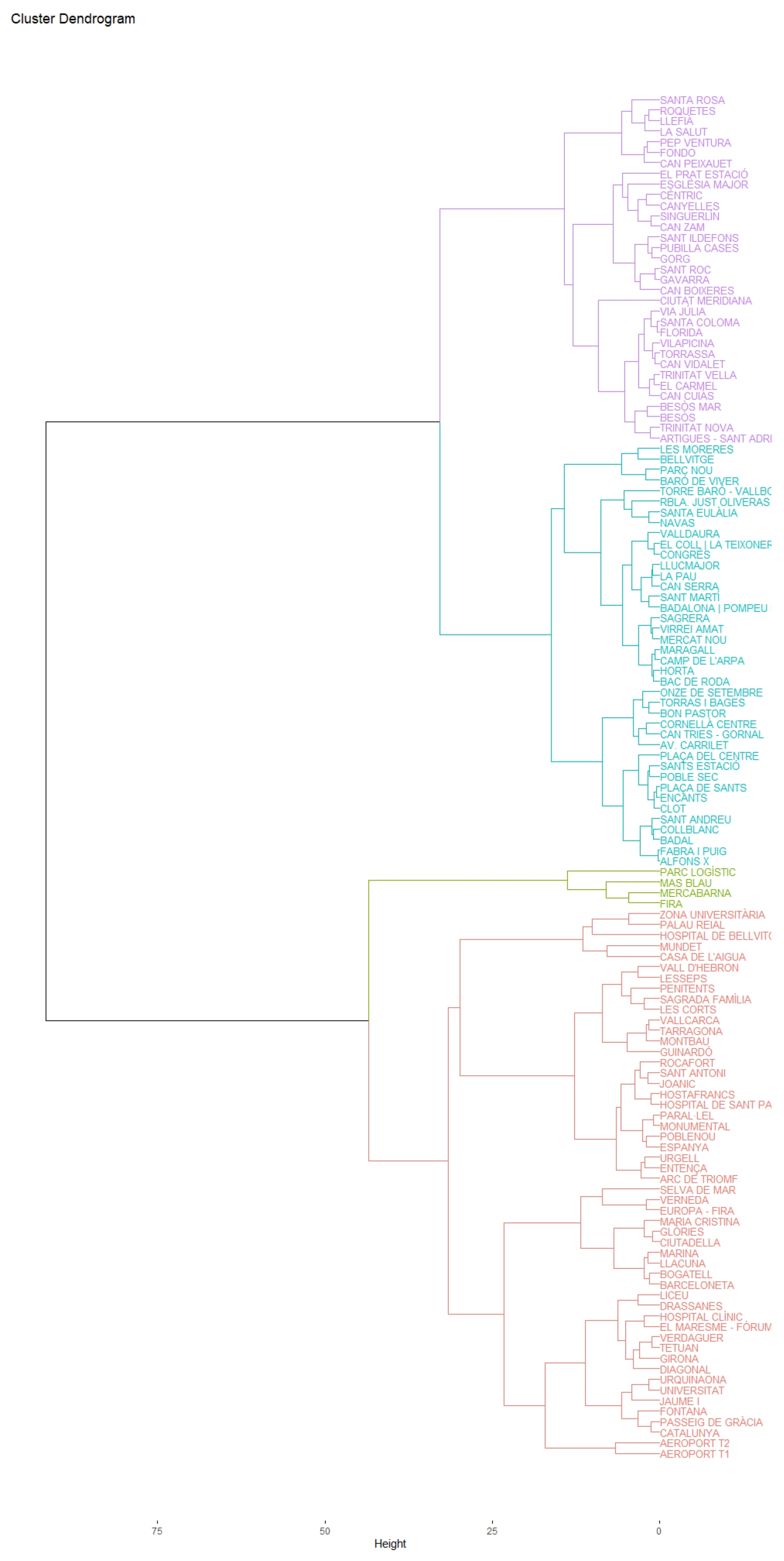
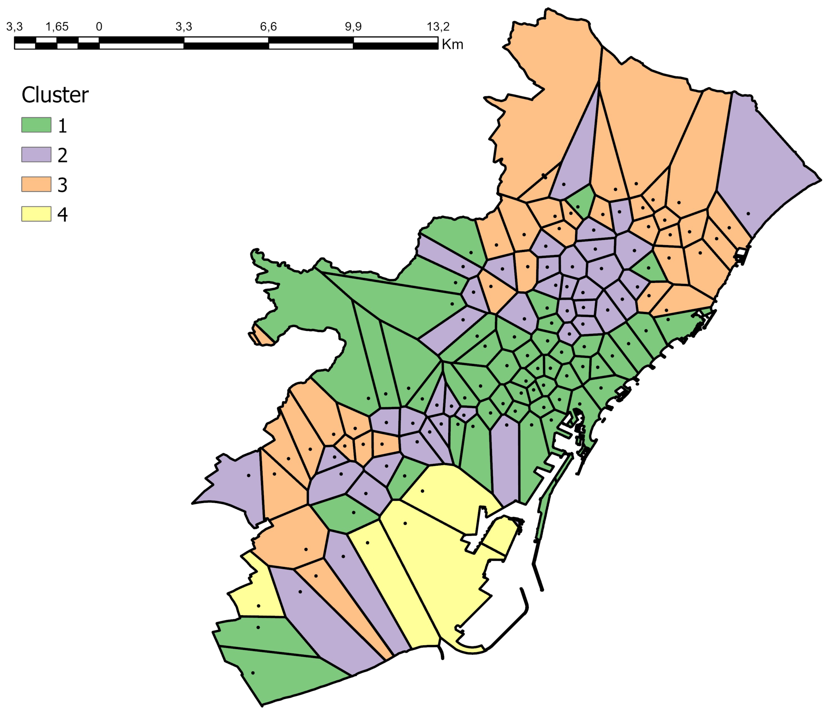
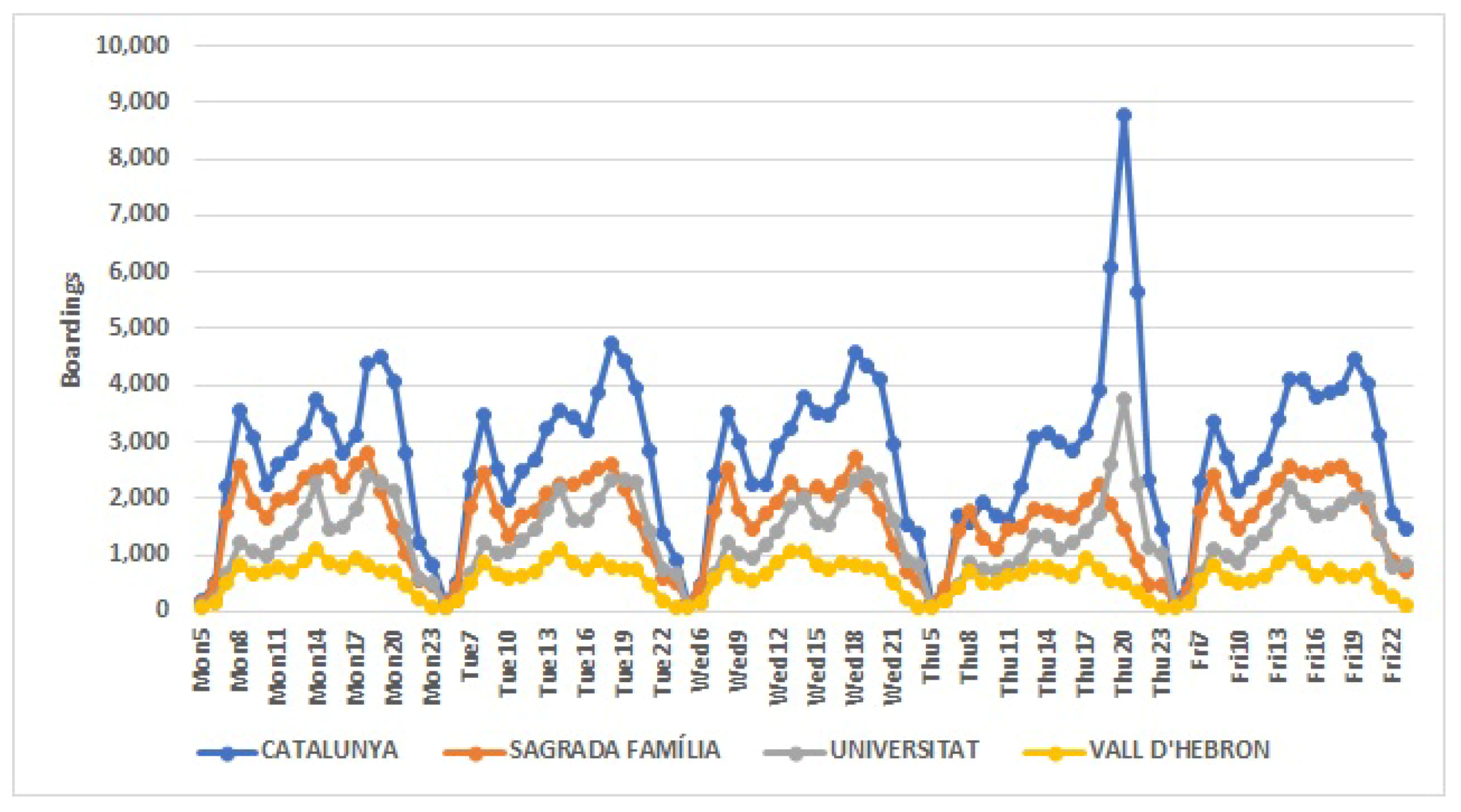
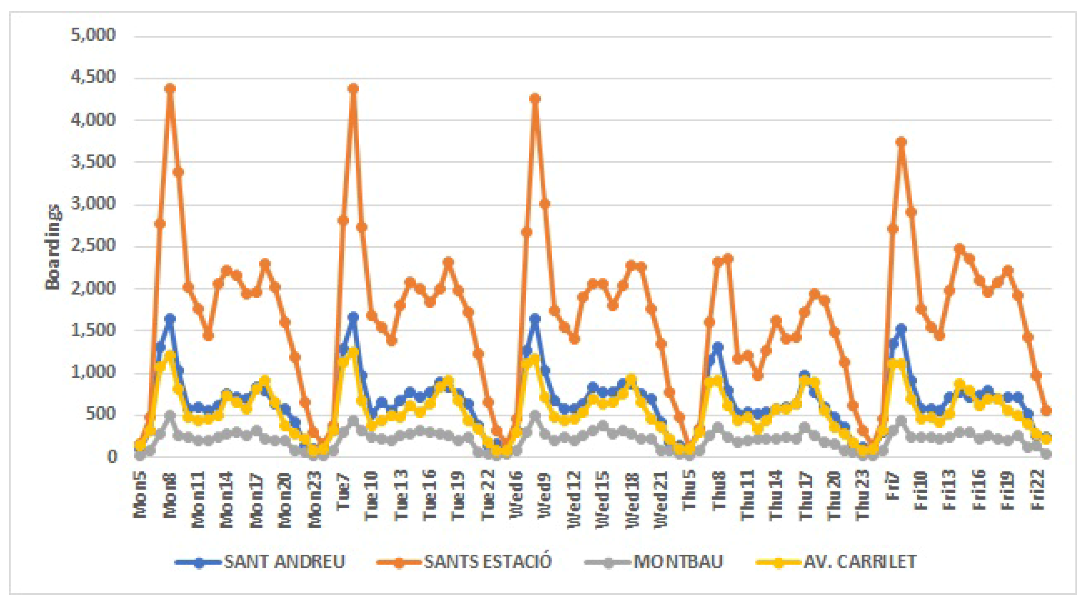
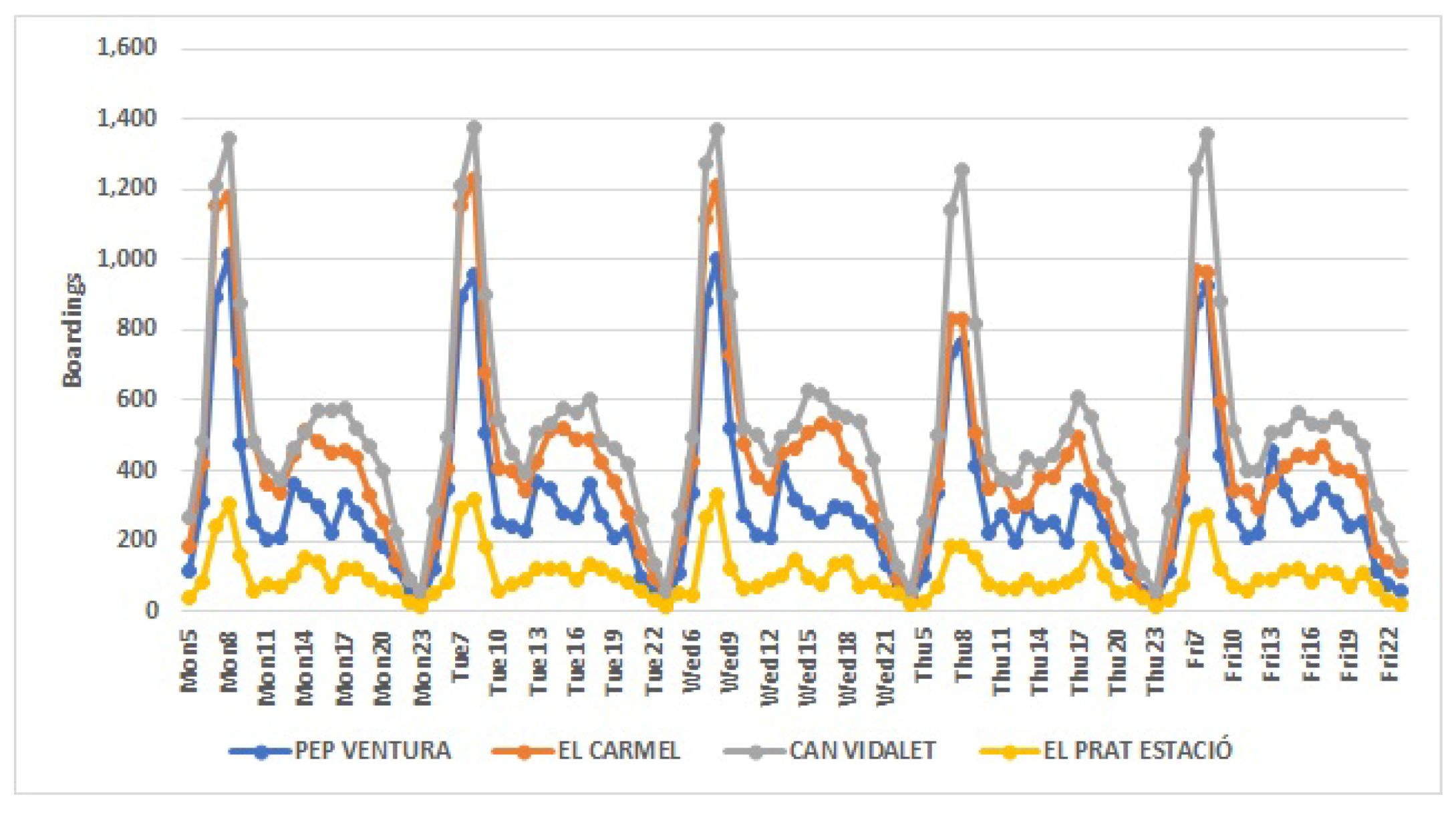
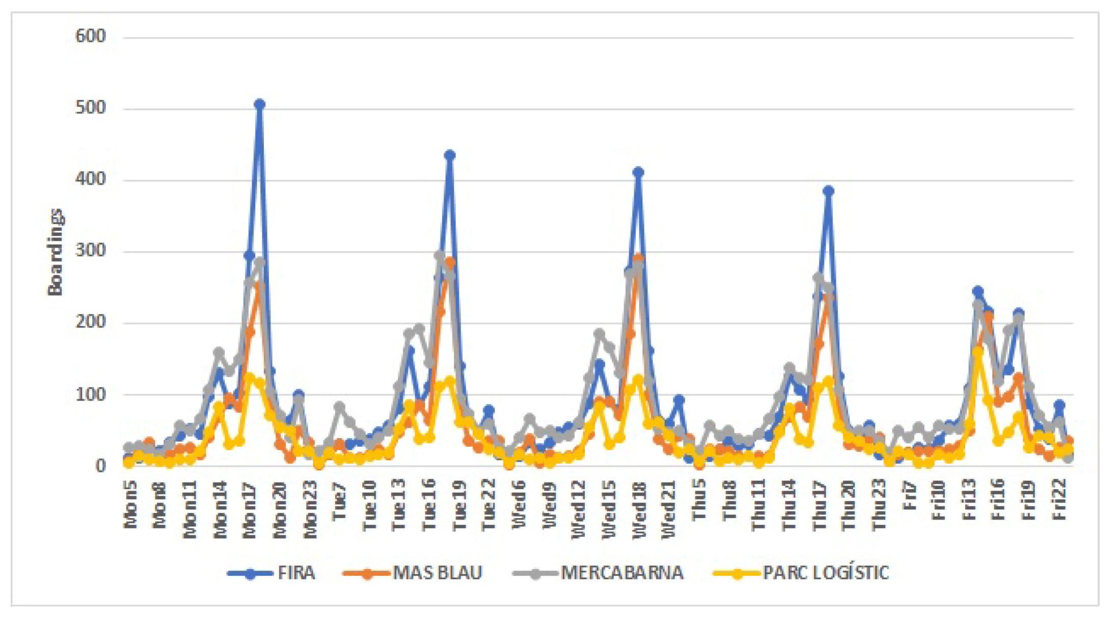
The cluster analysis carried out revealed, for working days, the existence of four groups with similar characteristics. The first conglomerate gathers the stations of the downtown area, the most touristic and monumental. In the second cluster, the stations that surround the center of Barcelona are grouped. They are, mainly, traditional and residential neighborhoods. The periphery stations, which link the center with the nearest municipalities, are those found in the third cluster. In the fourth cluster, the stations of the fairgrounds, large markets and logistics parks appear. Within each cluster, one can see the same pattern of behavior that reflects the similarities of the stations that form it, as can be seen at peak times, which differ between clusters.

The patterns observed reflect the daily activities of the urban area of Barcelona, which are related to the spatial structuring of the city and its characteristics, and are highly correlated with general daily routines.

The results of this work provide relevant information for the “Transports Metropolitan of Barcelona” company for public transport planning. These studies allow us to discover patterns of behavior needed to make decisions to improve the metro service. Nowadays, in the new post-pandemic normality, it is imperative to travel safely so as to stop the coronavirus spreading. It is important to avoid rush hours travels; people may choose to get on and off at subway stations with fewer travelers and do part of their journey by foot. Moreover, it is the task of public transport companies to increase the number of subway cars at a certain time if it gets too crowded, improve the infrastructure of stations with high passenger flow and reduce the time in-between metro services, among other security measures. For instance, the station “Sant Andreu”, from Cluster 2, has the highest number of passengers between 7:00 and 8:00 a.m., and, therefore, it is one of the stations where increasing the number of subway cars or the frequency of the service would be imperative. On the other hand, the station “Fira”, from Cluster 4, has peak hours at 14:00, 17:00 and 18:00 (p.m.), although with a much smaller number of passengers than “Sant Andreu”, and, thus, depending on the capacity of the station, the measures may not be as crucial as in the first one.

Future work involves relating these results to population, climate and economic variables that reflect other social circumstances that may influence the characteristics of the metro network stations. Moreover, annual data shall be analyzed to detect seasonality in behavior patterns. Further lines of investigations will also include a structural and robustness analysis of the network, using complex network analysis to determine critical nodes using different centrality measures. In addition, a detailed analysis of the structural characteristics of this subway network considering other different topological representations such as reduced L-space, P-space, C-space, etc. must be tackled. In addition, a theoretical framework must be proposed in which the notion of “subway line” is used as the basis to define new structural and robustness coefficients. Furthermore, additional transport lines (light rail network, bus network, etc.), can be considered in the analysis to obtain more realistic results. It would also be interesting to analyze the data post-COVID-19 and compare how the use of the public transport has changed, once the data become available.

References

1. Pternea, M.; Kepaptsoglou, K.; Karlaftis, M.G. Sustainable urban transit network design. Transp. Res. Part A Policy Pract. 2015, 77, 276–291. [Google Scholar] [CrossRef]
2. Latora, V.; M, M. Is the Boston subway a small-world network? Phys. A 2002, 314, 109–113. [Google Scholar] [CrossRef] [Green Version]
3. Lu, H.P.; Shi, Y. Complexity of public transport network. Tsinghua Sci. Technol. 2007, 12, 204–213. [Google Scholar] [CrossRef]
4. Zhang, J.H.; Zhao, M.W.; Liu, H.K.; Xu, X.M. Networked characteristics of the urban rail transit networks. Phys. A 2013, 392, 1538–1546. [Google Scholar] [CrossRef]
5. Liu, Z.; Song, R. Reliability analysis of Guangzhou subway with complex network theory. J. Transp. Syst. Eng. Inf. Technol. 2010, 10, 194–200. [Google Scholar]
6. Cats, O. Topological evolution of a metropolitan rail transport network: The case of Stockholm. J. Transp. Geogr. 2017, 62, 172–183. [Google Scholar] [CrossRef] [Green Version]
7. Derrible, S.; Kennedy, C. The complexity and robustness of metro networks. Phys. A 2010, 389, 3678–3691. [Google Scholar] [CrossRef]
8. Wang, X.; Koc, Y.; Derrible, S.; Ahmad, S.N.; Kooij, R.E. Multi-criteria robustness analysis of metro networks. Phys. A 2017, 474, 19–31. [Google Scholar] [CrossRef]
9. Zhang, J.H.; Xu, X.M.; Hong, L.; Wang, S.; Fei, Q. Networked analysis of the Shanghai subway network, in China. Phys. A 2011, 390, 4562–4570. [Google Scholar] [CrossRef]
10. Forero-Ortiz, E.; Martinez-Gomariz, E.; Canas Porcuna, M.; Locatelli, L.; Russo, B. Flood Risk Assessment in an Underground Railway System under the Impact of Climate Change-A Case Study of the Barcelona Metro. Sustainability 2020, 12, 5291. [Google Scholar] [CrossRef]
11. De Bona, A.; de Oliveira Rosa, M.; Ono Fonseca, K.; Lüders, R. A reduced model for complex network analysis of public transportation systems. Phys. A Stat. Mech. Its Appl. 2021, 567, 125715. [Google Scholar] [CrossRef]
12. Wang, Y.; Tian, C. Measure Vulnerability of Metro Network under Cascading Failure. IEEE Access 2021, 9, 683–692. [Google Scholar] [CrossRef]
13. Dempsey, P.S. Privacy Issues with the Use of Smart Cards; The National Academies Press: Washington, DC, USA, 2007. [Google Scholar]
14. Pelletier, M.P.; Trépanier, M.; Morency, C. Smart card data use in public transit: A literature review. Transp. Res. Part C Emerg. Technol. 2011, 19, 557–568. [Google Scholar] [CrossRef]
15. Li, T.; Sun, D.; Jing, P.; Yang, K. Smart card data mining of public transport destination: A literature review. Information 2018, 9, 18. [Google Scholar] [CrossRef] [Green Version]
16. Alsger, A.; Tavassoli, A.; Mesbah, M.; Ferreira, L.; Hickman, M. Public transport trip purpose inference using smart card fare data. Transp. Res. Part C Emerg. Technol. 2018, 87, 123–137. [Google Scholar] [CrossRef]
17. Alexander, L.; Jiang, S.; Murga, M.; González, M.C. Origin-destination trips by purpose and time of day inferred from mobile phone data. Transp. Res. Part C Emerg. Technol. 2015, 58, 240–250. [Google Scholar] [CrossRef]
18. Jun, C.; Dongyuan, Y. Estimating smart card commuters origin-destination distribution based on APTS data. J. Transp. Syst. Eng. Inf. Technol. 2013, 13, 47–53. [Google Scholar] [CrossRef]
19. Gonzalez, M.C.; Hidalgo, C.A.; Barabasi, A.L. Understanding individual human mobility patterns. Nature 2008, 453, 779–782. [Google Scholar] [CrossRef]
20. Briand, A.S.; Côme, E.; Trépanier, M.; Oukhellou, L. Analyzing year-to-year changes in public transport passenger behaviour using smart card data. Transp. Res. Part C Emerg. Technol. 2017, 79, 274–289. [Google Scholar] [CrossRef]
21. El Mahrsi, M.K.; Come, E.; Oukhellou, L.; Verleysen, M. Clustering Smart Card Data for Urban Mobility Analysis. IEEE Trans. Intell. Transp. Syst. 2017, 18, 712–728. [Google Scholar] [CrossRef]
22. Chen, C.; Chen, J.; Barry, J. Diurnal pattern of transit ridership: A case study of the New York City subway system. J. Transp. Geogr. 2009, 17, 176–186. [Google Scholar] [CrossRef]
23. Wang, W.; Lo, S.; Liu, S. Aggregated metro trip patterns in urban areas of Hong Kong: Evidence from automatic fare collection records. J. Urban Plan. Dev. 2015, 141, 05014018. [Google Scholar] [CrossRef]
24. Kim, M.K.; Kim, S.P.; Heo, J.; Sohn, H.G. Ridership patterns at subway stations of Seoul capital area and characteristics of station influence area. KSCE J. Civ. Eng. 2017, 21, 964–975. [Google Scholar] [CrossRef]
25. Ding, C.; Cao, X.; Liu, C. How does the station-area built environment influence Metrorail ridership? Using gradient boosting decision trees to identify non-linear thresholds. J. Transp. Geogr. 2019, 77, 70–78. [Google Scholar] [CrossRef]
26. Langlois, G.G.; Koutsopoulos, H.N.; Zhao, J. Inferring patterns in the multi-week activity sequences of public transport users. Transp. Res. Part C Emerg. Technol. 2016, 64, 1–16. [Google Scholar] [CrossRef] [Green Version]
27. Lu, Y.; Zhang, Y. Toward a Stakeholder Perspective on Safety Risk Factors of Metro Construction: A Social Network Analysis. Complexity 2020, 2020, 8884304. [Google Scholar] [CrossRef]
28. Zhou, C.; Kong, T.; Jiang, S.; Chen, S.; Zhou, Y.; Ding, L. Quantifying the evolution of settlement risk for surrounding environments in underground construction via complex network analysis. Tunn. Undergr. Space Technol. 2020, 103, 103490. [Google Scholar] [CrossRef]
29. Niu, K.; Fang, W.; Song, Q.; Guo, B.; Du, Y.; Chen, Y. An Evaluation Method for Emergency Procedures in Automatic Metro Based on Complexity. IEEE Trans. Intell. Transp. Syst. 2021, 22, 370–383. [Google Scholar] [CrossRef]
30. Chen, S.; Zhuang, D. Evolution and evaluation of the Guangzhou metro network topology based on an integration of complex network analysis and GIS. Sustainability 2020, 12, 538. [Google Scholar] [CrossRef] [Green Version]
31. Bernal, E.; del Rey, A.; Villardón, P. Analysis of madrid metro network: From structural to HJ-biplot perspective. Appl. Sci. 2020, 10, 5689. [Google Scholar] [CrossRef]
32. Moreno-Pulido, S.; Pavón-Domínguez, P.; Burgos-Pintos, P. Temporal evolution of multifractality in the Madrid Metro subway network. Chaos Solitons Fractals 2021, 142, 110370. [Google Scholar] [CrossRef]
33. Meng, Y.; Tian, X.; Li, Z.; Zhou, W.; Zhou, Z.; Zhong, M. Exploring node importance evolution of weighted complex networks in urban rail transit. Phys. A: Stat. Mech. Its Appl. 2020, 558, 124925. [Google Scholar] [CrossRef]
34. Yu, W.; Ye, X.; Chen, J.; Yan, X.; Wang, T. Evaluation indexes and correlation analysis of origination-destination travel time of Nanjing metro based on complex network method. Sustainability 2020, 12, 1113. [Google Scholar] [CrossRef] [Green Version]
35. Wang, J.; Ren, J.; Fu, X. Research on Bus and Metro Transfer from Perspective of Hypernetwork- A Case Study of Xi’an, China (December 2020). IEEE Access 2020, 8, 227048–227063. [Google Scholar] [CrossRef]
36. Wang, W.; Wang, Y.; Correia, G.; Chen, Y. A Network-Based Model of Passenger Transfer Flow between Bus and Metro: An Application to the Public Transport System of Beijing. J. Adv. Transp. 2020, 2020, 6659931. [Google Scholar] [CrossRef]
37. Han, Y.; Wang, S.; Ren, Y.; Wang, C.; Gao, P.; Chen, G. Predicting Station-Level Short-Term Passenger Flow in a Citywide Metro Network Using Spatiotemporal Graph Convolutional Neural Networks. ISPRS Int. J. Geo-Inf. 2019, 8, 243. [Google Scholar] [CrossRef] [Green Version]
38. Huh, J.; Seo, Y. Understanding Edge Computing: Engineering Evolution With Artificial Intelligence. IEEE Access 2019, 7, 164229–164245. [Google Scholar] [CrossRef]
39. Li, W.; Luo, Q.; Cai, Q. A Smart Path Recommendation Method for Metro Systems with Passenger Preferences. IEEE Access 2020, 8, 20646–20657. [Google Scholar] [CrossRef]
40. Bakıcı, T.; Almirall, E.; Wareham, J. A smart city initiative: The case of Barcelona. J. Knowl. Econ. 2013, 4, 135–148. [Google Scholar] [CrossRef]
41. Kolaczyk, E.D. Statistical Analysis of Network Data; Springer Science+Business Media: Berlin/Heidelberg, Germany, 2009. [Google Scholar]
42. Barabási, A.L. Network Science; Cambridge University Press: Cambridge, UK, 2016. [Google Scholar]
43. Van Mieghem, P. Graph Spectra for Complex Networks; Cambridge University Press: Cambridge, UK, 2011. [Google Scholar]
44. Newman, M.E.J. Networks: An Introduction; Oxford University Press: Oxford, UK, 2010. [Google Scholar]
45. Wu, J.; Barahona, M.; Tan, Y.J.; Deng, H.Z. Spectral measure of structural robustness in complex networks. IEEE Trans. Syst. Man Cybern. Part A 2011, 41, 1244–1252. [Google Scholar] [CrossRef]
46. Li, C.; Wang, H.; de Haan, W.; J, S.C.; Van Mieghem, P. The correlation of metrics in complex networks with applications in functional brain networks. J. Stat. Mech. Theory Exp. 2011, 2011, P11018. [Google Scholar] [CrossRef] [Green Version]
47. Jolliffe, I.T.; Cadima, J. Principal component analysis: A review and recent developments. Philos. Trans. R. Soc. A Math. Phys. Eng. Sci. 2016, 374, 20150202. [Google Scholar] [CrossRef] [PubMed]
48. Dunteman, G.H. Principal Components Analysis; Number 69 in Quantitative Applications in the Social Sciences; Sage Publications: Thousand Oaks, CA, USA, 1989. [Google Scholar]
49. Govender, P.; Sivakumar, V. Application of k-means and hierarchical clustering techniques for analysis of air pollution: A review (1980–2019). Atmos. Pollut. Res. 2020, 11, 40–56. [Google Scholar] [CrossRef]
50. Johnson, S.C. Hierarchical clustering schemes. Psychometrika 1967, 32, 241–254. [Google Scholar] [CrossRef]
51. Bouguettaya, A.; Yu, Q.; Liu, X.; Zhou, X.; Song, A. Efficient agglomerative hierarchical clustering. Expert Syst. Appl. 2015, 42, 2785–2797. [Google Scholar] [CrossRef]
52. Day, W.H.; Edelsbrunner, H. Efficient algorithms for agglomerative hierarchical clustering methods. J. Classif. 1984, 1, 7–24. [Google Scholar] [CrossRef]
53. Ward, J.H., Jr. Hierarchical grouping to optimize an objective function. J. Am. Stat. Assoc. 1963, 58, 236–244. [Google Scholar] [CrossRef]
54. Mojena, R. Hierarchical grouping methods and stopping rules: An evaluation. Comput. J. 1977, 20, 359–363. [Google Scholar] [CrossRef] [Green Version]
55. Blashfield, R.K. Mixture model tests of cluster analysis: Accuracy of four agglomerative hierarchical methods. Psychol. Bull. 1976, 83, 377. [Google Scholar] [CrossRef]
56. Murtagh, F.; Legendre, P. Ward’s hierarchical agglomerative clustering method: Which algorithms implement Ward’s criterion? J. Classif. 2014, 31, 274–295. [Google Scholar] [CrossRef] [Green Version]
57. Kaufman, L.; Rousseeuw, P.J. Finding Groups in Data: An Introduction to Cluster Analysis; John Wiley & Sons: Hoboken, NJ, USA, 2009; Volume 344. [Google Scholar]
58. Wu, X.; Tse, C.; Dong, H.; Ho, I.; Lau, F. A Network Analysis of World’s Metro Systems. In Proceedings of the 2016 International Symposium on Nonlinear Theory and Its Applications (NOLTA2016), Yugawara, Japan, 27–30 November 2016; The Institute of Electronics, Information and Communication Engineers: Tokyo, Japan, 2016; pp. 606–609. [Google Scholar]
59. Frutos Bernal, E.; Martín del Rey, A. Study of the Structural and Robustness Characteristics of Madrid Metro Network. Sustainability 2019, 11, 3486. [Google Scholar] [CrossRef] [Green Version]
60. RStudio Team. RStudio: Integrated Development Environment for R; RStudio, PBC: Boston, MA, USA, 2020. [Google Scholar]
Figure 1. The 2019 Barcelona subway (Available online: https://www.metrobarcelona.es/mapas.html (accessed on 15 February 2021)).
Electronics 10 00557 g001
Figure 2. Pearson’s correlation coefficients of daily ridership.
Electronics 10 00557 g002
Figure 3. Time-varying diagram of passenger flow (total counts of boarding).
Electronics 10 00557 g003
Figure 4. Heatmap with the total number of validations per hour for 35 randomly selected stations.
Electronics 10 00557 g004
Figure 5. Passenger flow boxplots.
Electronics 10 00557 g005
Figure 6. The graph representing the Barcelona subway network using Mathematica.
Electronics 10 00557 g006
Figure 7. Degree distribution of Barcelona subway network.
Electronics 10 00557 g007
Figure 8. Cumulative degree distribution of Barcelona subway network.
Electronics 10 00557 g008
Figure 9. Total variance explained by each principal component (weekdays).
Electronics 10 00557 g009
Figure 10. Contributions (top) and correlation (bottom) for the first three components.
Electronics 10 00557 g010
Figure 11. Clusters: Hierarchical clustering.
Electronics 10 00557 g011
Figure 12. Map of the different stations colored by cluster (weekdays).
Electronics 10 00557 g012
Figure 13. Pattern of boardings in stations of Cluster 1 (weekdays).
Electronics 10 00557 g013
Figure 14. Pattern of boarding in stations of Cluster 2 (weekdays).
Electronics 10 00557 g014
Figure 15. Pattern of boarding in stations of Cluster 3 (weekdays).
Electronics 10 00557 g015
Figure 16. Pattern of boarding stations of Cluster 4 (weekdays).
Electronics 10 00557 g016