Segmentation of Aorta 3D CT Images Based on 2D Convolutional Neural Networks

Abstract

The automatic segmentation of the aorta can be extremely useful in clinical practice, allowing the diagnosis of numerous pathologies to be sped up, such as aneurysms and dissections, and allowing rapid reconstructive surgery, essential in saving patients’ lives. In recent years, the success of Deep Learning (DL)-based decision support systems has increased their popularity in the medical field. However, their effective application is often limited by the scarcity of training data. In fact, collecting large annotated datasets is usually difficult and expensive, especially in the biomedical domain. In this paper, an automatic method for aortic segmentation, based on 2D convolutional neural networks (CNNs), using 3D CT (computed axial tomography) scans as input is presented. For this purpose, a set of 153 CT images was collected and a semi-automated approach was used to obtain their 3D annotations at the voxel level. Although less accurate, the use of a semi-supervised labeling technique instead of a full supervision proved necessary to obtain enough data in a reasonable amount of time. The 3D volume was analyzed using three 2D segmentation networks, one for each of the three CT views (axial, coronal and sagittal). Two different network architectures, U-Net and LinkNet, were used and compared. The main advantages of the proposed method lie in its ability to work with a reduced number of data even with noisy targets. In addition, analyzing 3D scans based on 2D slices allows for them to be processed even with limited computing power. The results obtained are promising and show that the neural networks employed can provide accurate segmentation of the aorta.

1. Introduction

In recent years, the use of Deep Learning (DL) has improved the state of the art in many different fields, ranging from computer vision [1,2,3] and text analysis [4,5,6] to bioinformatics [7,8]. More specifically, DL-based decision support systems have become increasingly popular in the medical field [9]—and in particular for application in the Internet of Medical Things—where CNNs have been successfully employed for the classification of radiological, magnetic resonance or CT (Computerized Axial Tomography) images [10,11] and for natural images, for instance, in the classification of atypical nevi and melanomas [12,13,14], for the segmentation of bacterial colonies grown on Petri plates [15,16] and for retinal images [17]. In this paper, a DL aortic image semantic segmentation system is presented. The automatic segmentation tool was developed based on a new proprietary dataset, collected at the Department of Medicine, Surgery and Neuroscience of the University of Siena (Italy).

The aorta is the most important arterial vessel in the human body and is responsible for transporting blood from the heart to all other organs. It originates from the left ventricle and extends throughout the abdomen, where it divides into the iliac arteries. The aorta can be classified according to its anatomical location [18,19] in the thoracic aorta and the abdominal aorta. Depending on its morphology and on the direction of blood flow, the different parts of the aorta are also classified as ascending/descending and the aortic arch. Normally, the average aortic diameter does not exceed 2.5 cm, but over time it can dilate, stiffen or deform due to various pathologies, such as aneurysms [20] and dissections [21]. An aortic aneurysm is a permanent and non-physiological dilation of the aorta, where the vessel diameter exceeds the normal one by more than 1.5 cm. Aortic aneurysms are linked to a high mortality rate and are difficult to treat because they make the vascular wall of the dilated segment thinner and more prone to rupture. In addition, vessel dilation alters the blood flow, promoting abnormal blood clots (emboli) or thrombi. Instead, aortic dissection is a serious condition in which there is a tear in the aortic wall. When the tear extends along the wall, blood can flow between the layers of the aortic wall, resulting in a false lumen. This can lead to rupture of the vessel or a decrease in blood flow to the organs (ischemia).

The automated segmentation of the aorta from CT images helps clinicians speed up the diagnosis of these pathologies, enabling rapid reconstructive surgery, which is critical to saving patients’ lives. The purpose of image segmentation is to divide a digital image into multiple segments based on certain visual features (which characterize the whole segment). In particular, image semantic segmentation can be viewed as a pixel-wise (voxel in 3D images) classification, in which a label is assigned to each pixel/voxel. This is an important step in image understanding, because it provides a complete characterization of the objects present in the image. In recent years, several semantic segmentation models, based on deep neural networks, have been proposed [22,23,24,25,26]. DL architectures are usually trained through supervised learning, exploiting large sets of labeled data, which are commonly publicly available. Such datasets are used to train generic semantic segmentation networks, which can later be adapted to specific domains with less data. Unfortunately, no publicly available aortic datasets which can be used for this purpose exist. For this reason, in collaboration with the Department of Medicine, Surgery and Neuroscience of the University of Siena, a dataset of 154 3D CT images was collected. In each image, all pixels belonging to the aorta were labeled using a semi-automatic approach. Labeling images is, in fact, an extremely time consuming task. Therefore, even if labels obtained in a semi-automatic way provide a lower quality information this was a necessary trade-off to obtain enough data in a reasonable amount of time. Subsequently, following an approach inspired by [10], the segmented images were employed to train three 2D CNN segmentation models, one for each view (coronal, sagittal and axial). Several architectures based on both LinkNet [27] and U-Net [28] were employed as segmentation networks and their results were compared. Two-dimensional models were preferred to three-dimensional for computational reasons and also to reduce overfitting—with a small number of images available, in fact, training a 3D model would be difficult due to the large number of parameters required by convolutions. The results obtained are very promising and show that, even with the use of low-quality labeled images, DL architectures can successfully segment the aorta from CT scans.

In particular, the main contributions of this manuscript can be summarized as:

• A new approach for 3D CT scan segmentation is proposed for aorta images, based on 2D CNNs;
• The model has low computational requirements and can also be employed with limited computational resources;
• The approach can be employed on small datasets, possibly with noisy labels;
• The method was tested on an original dataset collected at the University of Siena not publicly available due to privacy issues.

The paper is organized as follows. In Section 2, the related literature is reviewed. Section 3 presents a description of the proposed approach, and Section 4 discusses the obtained experimental results. Finally, Section 5 draws some conclusions and future perspectives.

Table A1. Nomenclature Table.

Acronym	Meaning
CNN	Convolutional Neural Network
CT	Computerized Axial Tomography
DICOM	Digital Imaging and Communications in Medicine
AHE	Adaptive Histogram Equalization
ML	Machine Learning
DL	Deep Learning

in Appendix A summarizes the nomenclature used throughout the manuscript.

2. Related Works

2.1. Natural Image Segmentation

In recent years, many advances were made in image semantic segmentation of natural scenes using deep fully convolutional neural networks [22,23,24,25,26]. Usually, these architectures are based on an encoder–decoder structure. On the one hand, the encoder extracts a high-level representation of the input image by employing subsequent layers of convolutions and down-sampling. On the other hand, the decoder produces a representation at the image level by recovering the original spatial resolution. Supervised training of these architectures requires pixel-level labeling, which is often time consuming and difficult to obtain, especially in medical image processing, where often, available datasets are too small. For this reason, in biomedical imaging, it is critical to use networks that effectively recover the input resolution while maintaining a small number of parameters. In this paper, U-Net [28] and LinkNet [27], two popular networks often employed in medical image semantic segmentation, were compared. U-Net consists of a convolutional encoder followed by a decoder composed of up-convolutions combined with skip-connections. Skip-connections concatenate specific feature maps in the encoder with feature maps at the same resolution in the decoder. In comparison, LinkNet [27] is a network architecture devised to reduce the number of parameters by efficiently sharing the information learnt by the encoder with the decoder. After each down-sampling block, feature maps from the encoder layer are summed up with feature maps of the corresponding decoder layer at the same resolution.

2.2. Computerized Axial Tomography Segmentation

Some tools such as ITK-SNAP [29] and 3D Slicer [30] allow one to manually segment or, alternatively, to obtain a semi-automatic segmentation of CT scans. The ITK-SNAP semi-automatic procedure uses an active contour method based on snakes. A snake is a spline that adapts its shape to the contours of an object while also trying to avoid discontinuities in the approximated curve. The obtained segmentation usually needs post-processing to reduce the noise and to be refined. Manual segmentation is more time consuming but gives accurate segments, while semi-automatic segmentation is slightly faster but often not so accurate. For this reason, the development of fully automated segmentation systems could provide an excellent alternative method for obtaining segmented images.

Recently, several methods based on DL were proposed for medical image segmentation. In [31], a fully automated system was proposed for the segmentation of abdominal organs, including the abdominal aorta. In particular, a feature-based approach was used to approximately localize the organ, while a 3D CNN was dedicated to segmentation. In [32], a fully automatic pipeline for thrombi detection was developed, where thrombus segmentation is performed on a single 2D slice—a method subsequently extended with the use of 3D convolutions in [33]. An automated method for segmenting the ascending aorta, the aortic arch and the descending aorta was proposed in [34]. A dilated convolutional neural network was applied separately to the axial, coronal and sagittal planes, with the final segmentation obtained by averaging the results on each view. In [35], instead, the aorta was located using a CNN-based classifier trained on image patches. After a first phase of detection, the edges of the aorta were extracted with the Circle Hough Transform algorithm and the lumen diameter was used to predict the risk of abdominal aneurysms. A multitask learning approach was used to segment the entire aorta, true lumen and false lumen using a 3D CNN in [36]. Finally, in [10], a fully automated pipeline was developed for the segmentation of the entire aorta, including the common iliac arteries, using 2D networks trained on axial, coronal and sagittal views. Similarly to [10], in this work, the aorta segmentation was obtained from three 2D networks trained on the axial, coronal and sagittal views.

3. Aorta Segmentation

In the following sections, the proposed aortic segmentation approach and its pipeline are described in Figure 1. In particular, in Section 3.1, the pre-processing steps (resampling of CT scans—available in DICOM format—normalization and extraction of slices for each view) are presented. Subsequently, segmentation models and their training are discussed in Section 3.2.

3.1. Pre-Processing

Preliminarily, each scan (and each corresponding label) was oriented in RAI (Right-to-left, Anterior-to-posterior, Inferior-to-superior) mode. The 3D volume was then resampled, normalizing the voxel to the size of 1 mm × 1 mm × 1 mm. The resampling process mapped the image from a given reference system, f, to a new coordinate system, m. It was defined by a lattice in the reference system, f, and by a transformation function, $T_f^m$, that mapped the points from f to m. Nearest-neighbor was used as the interpolation algorithm, so that any value assigned at any point in m equaled the nearest point in f. Adaptive Histogram Equalization (AHE) normalization was employed to reduce the variability of the scans, mainly caused by the different setups used during the acquisition process. AHE was applied over the entire CT scan and is a common technique used to enhance contrast and edges in images. The algorithm calculated a local histogram (see Equation (1)) for each sub–part of the image and, based on these histograms, the intensity values of the whole image were normalized:

$$g_{i,j}=floor((L-1)\sum _{n=0}^{f_{i,j}}{p}_n)$$

(1)

where g is the equalized sub-part of the image, $p_n$ is the normalized histogram and L is the maximum intensity of a pixel. Some slices normalized by AHE are reported in Figure 2.

After pre-processing, CT scans were cropped to reduce their size. This also allowed one to remove parts of the scan where the aorta was not present (normally, the entire scan goes from the pelvis to the head). The dimensions of the 3D bounding box were multiples of 32 (to have a final image size that fit the input of the chosen segmentation network without using padding). Finally, the slices for each view (coronal, sagittal and axial) were extracted and used for network training. An example of an axial slice together with its label is given in Figure 3.

3.2. Deep Segmentation Network Training

In this section, the training procedure employed to segment the aorta from 2D slices extracted from 3D CT scans is presented. In particular, two different networks were tested, U-Net [28] and LinkNet [27] (see Figure 4), which share an encoder–decoder architecture.

The encoder transforms the original image into a set of feature maps, whereas the decoder up-samples the encoded representation (which typically has a lower resolution due to a series of down-sampling operations) to restore the size of the original input. The main difference between U-Net and LinkNet resides in the decoding structure. In particular, while U-Net concatenates the encoder and decoder feature maps, LinkNet simply adds the corresponding feature maps. In this work, two encoder models, pre-trained on ImageNet [37], ResNet34 [38] and Inception ResNet V2 [39], were used. The Inception ResNet V2 is deeper than the ResNet34 and usually provides better performance. The reduced number of parameters of ResNet34 can guarantee a better generalization on small datasets (such as the one proposed in this paper). The pseuodocode of the training procedure is reported in Algorithm 1.

Algorithm 1: Training phase pseudocode

Three networks, one for each view of the CT scans, were trained using a linear combination of binary cross entropy [40] and Jaccard error as the loss function (see Equations (2)–(4) for the definitions):

$$L_{bce}(gt,pr)=-gt·log\left(pr\right)-(1-gt)·log(1-pr)$$

(2)

$$L_{jac}(gt,pr)=1-\frac{gt\cap pr}{gt\cup pr}$$

(3)

$$L(gt,pr)=L_{bce}+L_{jac}$$

(4)

where $pr$ is the network prediction and $gt$ is the ground truth. Moreover, Adam optimizer [41] and early stopping were employed on the validation set to avoid overfitting. To augment the number of training samples, data augmentation strategies (horizontal and vertical shift, max 10 px, and rotations, max 5°) were employed during training. The results obtained with the different models were compared using the Mean Intersection over Union (MIoU) on the validation set. The test set was then used as an hold-out set to assess the quality of the best model.

4. Experiments and Results

The dataset used in our experiments is described in Section 4.1, while the experimental setup and the obtained results are discussed in Section 4.2.

4.1. Dataset

The dataset, collected at the Department of Medicine, Surgery and Neuroscience of the University of Siena, is made up of 154 CT scans acquired with contrast medium. The scans were saved in DICOM (Digital Imaging and Communications in Medicine) format, which is the standard for CT images. The DICOM format requires the presence of a set of files, one for each slice, which collectively describe a 3D volume, together with a dictionary of metadata, that contains information on the acquisition setup and on the patient (patient data were anonymized; only details about their age and gender were kept).

Table 1. Dataset description.

Gender	Number of Scans	Average Age
Male	118	68.78 ± 12.99
Female	36	70.71 ± 11.24

reports the demographic description of the dataset as well as the number of CT scans available.

Additional metadata, which contain some descriptions of the collected CT scans, namely the orientation and size of the voxels, are available. The orientation is defined for each view: axial (X–Y plane), coronal (X–Z plane) and sagittal (Y–X plane), of the CT scans. Instead, the size of the voxel is defined by two parameters:

• The pixel spacing, which indicates the dimension in millimeters of a single pixel in each slice;
• The slice thickness, which corresponds to the distance in millimeters between two adjacent slices.

To train the deep segmentation model, the dataset was split into a training, validation and test set, as described in

Table 2. Size of the training, validation and test set.

Split	Number of CT Scans
Training	134
Validation	10
Test	10

.

All the scans were pre-processed as described in Section 3.1, resulting in a set of slices for each view of the scans.

Table 3. Number of slices for each view in the training, validation and test sets and relative dimensions.

Views	Training	Validation	Test	Dimension
Axial	39,465	2848	2675	$352\times 384$
Coronal	17,887	1196	1267	$352\times 736$
Sagittal	13,724	901	891	$384\times 736$

displays the number of slices belonging to the training, validation and test sets, along with their sizes, for each view.

Each slice of the dataset is grayscale, and each pixel has a binary label associated with it, indicating whether the pixel belongs to the aorta or not. Supervision is generated semi-automatically using 3DSlicer. The dataset shows high positional, labeling and contrast variability, mainly caused by the following reasons:

• Position of the aorta—not all the scans are centered in the same way;
• Presence of errors in the labels—the semi-automatic procedure used to create the labels is sometimes not accurate due to the presence of false positives (voxels which are labeled as aorta but that actually do not belong to it);
• Different acquisition systems—the CT scans were collected in different periods and using different acquisition systems.

4.2. Results and Discussion

As described before, different segmentation network architectures were tested. In particular, the following four architectures were used in our experiments:

• U-Net with ResNet34—U-Net architecture with ResNet34 used as the encoder;
• U-Net with Inception ResNet V2—U-Net architecture with Inception ResNet V2 used as the encoder;
• LinkNet with ResNet34—LinkNet architecture with ResNet34 used as the encoder;
• LinkNet with Inception ResNet V2—LinkNet architecture with Inception ResNet V2 used as the encoder.

For each of the above architectures, following the training procedure described in Section 3.2, three models were trained, one for each CT scan view (axial, coronal and sagittal). The results on the validation set of each model for each view are reported in

Table 4. Results of U-Net models on the validation set for axial, coronal and sagittal views.

Axial
Encoder	Loss	MIoU
ResNet34	0.3505	67.51%
InceptionResNetV2	0.2645	75.60%
Coronal
Encoder	Loss	MIoU
ResNet34	0.3191	70.98%
InceptionResNetV2	0.3186	70.86%
Sagittal
Encoder	Loss	MIoU
ResNet34	0.3652	67.94%
InceptionResNetV2	0.3029	73.06%

for U-Net and in

Table 5. Results of the LinkNet models on the validation set for axial, coronal and sagittal views.

Axial
Encoder	Loss	MIoU
ResNet34	0.1023	74.31%
InceptionResNetV2	0.0652	76.01%
Coronal
Encoder	Loss	MIoU
ResNet34	0.0845	73.68%
InceptionResNetV2	0.1082	72.98%
Sagittal
Encoder	Loss	MIoU
ResNet34	0.18	72.57%
InceptionResNetV2	0.0846	73.42%

for LinkNet, respectively.

As can be easily observed, LinkNet obtains a greater MIoU and, in particular, when the ResNet34 is used as the encoder, the difference between LinkNet and U-Net is greater. If, instead, Inception ResNet V2 is used as the encoder, the difference between U-Net and LinkNet is less significant. Furthermore, it can be noted that, even with a small dataset, Inception ResNet V2 outperforms ResNet34 in all the experiments. Only when the model is trained on the coronal view do the two architectures behave quite similarly. Based on these results, the LinkNet architecture with the Inception ResNet V2 encoder was chosen and evaluated on the test set. The results are reported in

Table 6. Results of the test set for the LinkNet model with Inception ResNet V2 as encoder.

InceptionResNetV2	MIoU
Axial	83.45%
Coronal	77.11%
Sagittal	76.75%

.

The results obtained are promising but limited by the quality of the annotations. Indeed, the ground truth of the dataset was obtained with a semi-automatic procedure and, in some cases, was not completely accurate. However, the dataset was provided with a reasonable supervision that somehow compensates for the absence of datasets with aortic images labeled at the pixel level. In Figure 5, some images are provided, together with their labels and the segmentation generated by the network, for a qualitative evaluation. 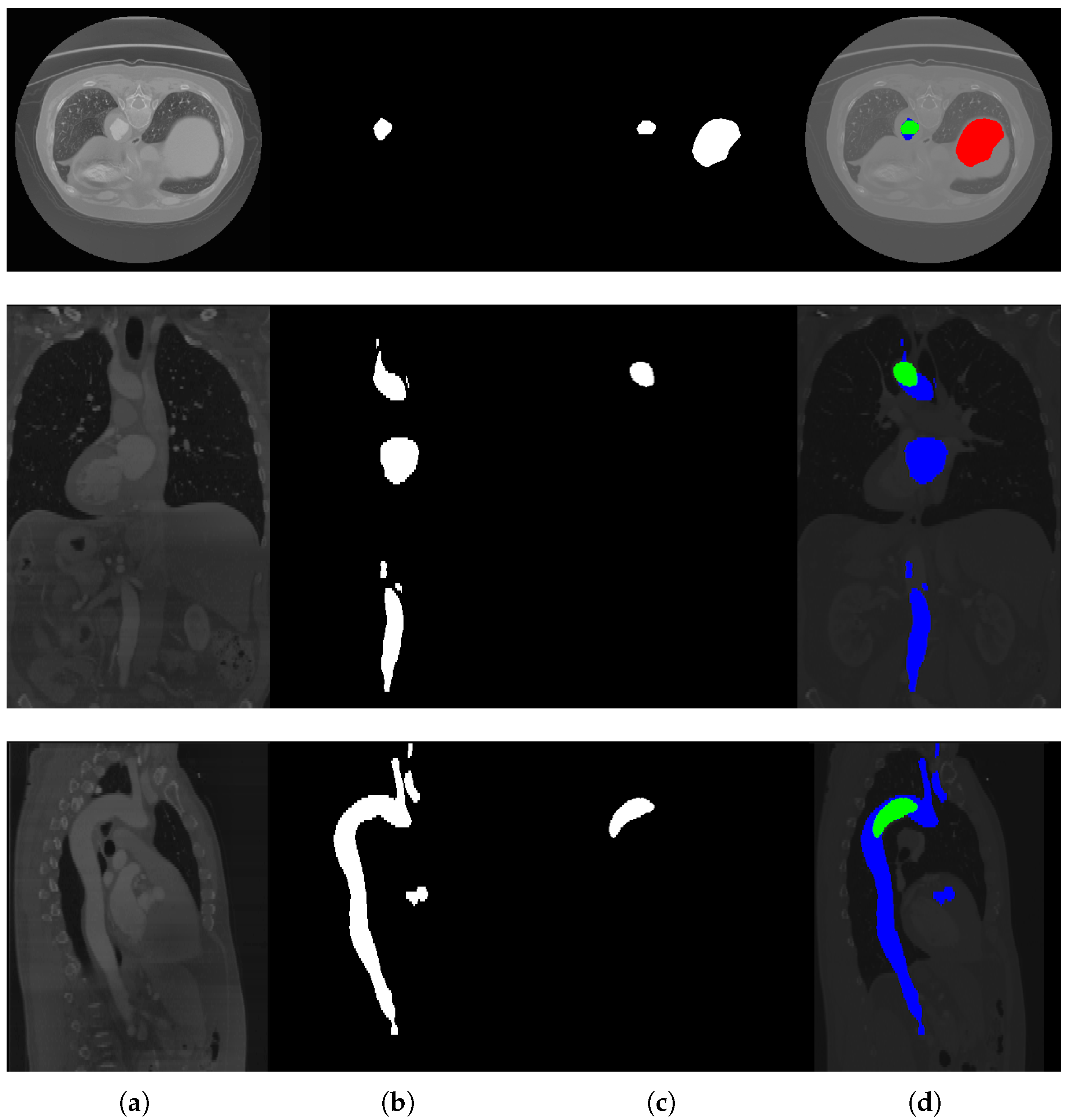Figure 6 shows some slices not correctly segmented by the network. As we can see, in this case, the images are actually difficult to interpret; in the second and third row, in fact, the slices are really dark and, in the first row, the network probably wrongly classified the aorta due to its size.

5. Conclusions

In this paper, some deep convolutional neural networks for aorta segmentation were trained, using a dataset of 154 CT scans collected at the Department of Medicine, Surgery and Neuroscience of the University of Siena. Two types of architectures, U-Net and LinkNet, with different types of encoders, ResNet34 and Inception ResNet V2, were tested as segmentation networks. Despite the fact that network training was based on a small set of training images with a low-quality supervision, obtained with a semi-automatic labeling approach, and there was variability in the acquisition conditions, we demonstrated that it was possible to successfully train three 2D segmentation networks, one for each view (axial, coronal and sagittal). Obtaining a set of high-quality supervised 3D images is costly and time consuming; however, if a larger set of semi-automatically supervised scans become available, it would be possible in principle to further improve the results. Therefore, as a matter of future research, we leave the possibility of employing a semi-supervised approach to enrich the current dataset, based on a set of unlabeled scans, that will hopefully increase the network performance. Another future development currently under investigation entails post-processing on the network output to clean the predictions. In particular, consistency between predictions from adjacent sections and between predictions from different views could be used to improve the segmentation quality.

References

1. Chéron, G.; Laptev, I.; Schmid, C. P-cnn: Pose-based cnn features for action recognition. In Proceedings of the IEEE International Conference on Computer Vision, Santiago, Chile, 7–13 December 2015; pp. 3218–3226. [Google Scholar]
2. He, K.; Gkioxari, G.; Dollár, P.; Girshick, R. Mask r-cnn. In Proceedings of the IEEE International Conference on Computer Vision, Venice, Italy, 22–29 October 2017; pp. 2961–2969. [Google Scholar]
3. Krizhevsky, A.; Sutskever, I.; Hinton, G.E. Imagenet classification with deep convolutional neural networks. Adv. Neural Inf. Process. Syst. 2012, 25, 1097–1105. [Google Scholar] [CrossRef]
4. Bonechi, S.; Andreini, P.; Bianchini, M.; Scarselli, F. COCO_TS dataset: Pixel–level annotations based on weak supervision for scene text segmentation. In Proceedings of the International Conference on Artificial Neural Networks, Munich, Germany, 17–19 September 2019; Springer: Cham, Switzerland, 2019; pp. 238–250. [Google Scholar]
5. Bonechi, S.; Bianchini, M.; Scarselli, F.; Andreini, P. Weak supervision for generating pixel–level annotations in scene text segmentation. Pattern Recognit. Lett. 2020, 138, 1–7. [Google Scholar] [CrossRef]
6. Vaswani, A.; Shazeer, N.; Parmar, N.; Uszkoreit, J.; Jones, L.; Gomez, A.N.; Kaiser, L.; Polosukhin, I. Attention is all you need. In Advances in Neural Information Processing Systems; Curran Associates, Inc.: Red Hook, NY, USA, 2017; pp. 5998–6008. [Google Scholar]
7. Jumper, J.; Evans, R.; Pritzel, A.; Green, T.; Figurnov, M.; Ronneberger, O.; Tunyasuvunakool, K.; Bates, R.; Žídek, A.; Potapenko, A.; et al. Highly accurate protein structure prediction with AlphaFold. Nature 2021, 596, 583–589. [Google Scholar] [CrossRef] [PubMed]
8. Pancino, N.; Rossi, A.; Ciano, G.; Giacomini, G.; Bonechi, S.; Andreini, P.; Scarselli, F.; Bianchini, M.; Bongini, P. Graph Neural Networks for the Prediction of Protein-Protein Interfaces. In ESANN; i6doc.com Inc.: Louvain-la-Neuve, Belgium, 2020; pp. 127–132. [Google Scholar]
9. Litjens, G.; Kooi, T.; Bejnordi, B.E.; Setio, A.A.A.; Ciompi, F.; Ghafoorian, M.; Van Der Laak, J.A.; Van Ginneken, B.; Sánchez, C.I. A survey on deep learning in medical image analysis. Med. Image Anal. 2017, 42, 60–88. [Google Scholar] [CrossRef] [PubMed] [Green Version]
10. Fantazzini, A.; Esposito, M.; Finotello, A.; Auricchio, F.; Pane, B.; Basso, C.; Spinella, G.; Conti, M. 3D automatic segmentation of aortic computed tomography angiography combining multi-view 2D convolutional neural networks. Cardiovasc. Eng. Technol. 2020, 11, 576–586. [Google Scholar] [CrossRef] [PubMed]
11. Rossi, A.; Vannuccini, G.; Andreini, P.; Bonechi, S.; Giacomini, G.; Scarselli, F.; Bianchini, M. Analysis of brain NMR images for age estimation with deep learning. Procedia Comput. Sci. 2019, 159, 981–989. [Google Scholar] [CrossRef]
12. Bonechi, S.; Bianchini, M.; Bongini, P.; Ciano, G.; Giacomini, G.; Rosai, R.; Tognetti, L.; Rossi, A.; Andreini, P. Fusion of visual and anamnestic data for the classification of skin lesions with deep learning. In Proceedings of the International Conference on Image Analysis and Processing, Trento, Italy, 9–10 September 2019; Springer: Cham, Switzerland, 2019; pp. 211–219. [Google Scholar]
13. Tognetti, L.; Bonechi, S.; Andreini, P.; Bianchini, M.; Scarselli, F.; Cevenini, G.; Moscarella, E.; Farnetani, F.; Longo, C.; Lallas, A.; et al. A new deep learning approach integrated with clinical data for the dermoscopic differentiation of early melanomas from atypical nevi. J. Dermatol. Sci. 2021, 101, 115–122. [Google Scholar] [CrossRef] [PubMed]
14. Połap, D. Analysis of skin marks through the use of intelligent things. IEEE Access 2019, 7, 149355–149363. [Google Scholar] [CrossRef]
15. Andreini, P.; Bonechi, S.; Bianchini, M.; Mecocci, A.; Scarselli, F. A deep learning approach to bacterial colony segmentation. In Proceedings of the International Conference on Artificial Neural Networks, Rhodes, Greece, 4–7 October 2018; Springer: Cham, Switzerland, 2018; pp. 522–533. [Google Scholar]
16. Andreini, P.; Bonechi, S.; Bianchini, M.; Mecocci, A.; Scarselli, F. Image generation by GAN and style transfer for agar plate image segmentation. Comput. Methods Programs Biomed. 2020, 184, 105268. [Google Scholar] [CrossRef] [PubMed]
17. Andreini, P.; Bonechi, S.; Bianchini, M.; Mecocci, A.; Scarselli, F.; Sodi, A. A two stage gan for high resolution retinal image generation and segmentation. arXiv 2019, arXiv:1907.12296. [Google Scholar]
18. Tortora, G.J.; Derrickson, B.H. Principles of Anatomy and Physiology; John Wiley & Sons: Hoboken, NJ, USA, 2018. [Google Scholar]
19. Tortora, G.J.; Petti, K. Principles of Human Anatomy; John Wiley & Sons: Hoboken, NJ, USA, 2002. [Google Scholar]
20. Society of NeuroInterventional Surgery. Aneurysms. Available online: https://www.nhlbi.nih.gov/health-topics/aneurysm (accessed on 25 May 2021).
21. Criado, F.J. Aortic dissection: A 250-year perspective. Tex. Heart Inst. J. 2011, 38, 694. [Google Scholar] [PubMed]
22. Chen, L.C.; Papandreou, G.; Schroff, F.; Adam, H. Rethinking atrous convolution for semantic image segmentation. arXiv 2017, arXiv:1706.05587. [Google Scholar]
23. Long, J.; Shelhamer, E.; Darrell, T. Fully convolutional networks for semantic segmentation. In Proceedings of the IEEE Conference on Computer Vision and Pattern Recognition, Boston, MA, USA, 7–12 June 2015; pp. 3431–3440. [Google Scholar]
24. Takikawa, T.; Acuna, D.; Jampani, V.; Fidler, S. Gated-SCNN: Gated Shape CNNs for Semantic Segmentation. In Proceedings of the 2019 IEEE/CVF International Conference on Computer Vision (ICCV), Seoul, Korea, 27–18 October 2019; pp. 5228–5237. [Google Scholar]
25. Wu, H.; Zhang, J.; Huang, K.; Liang, K.; Yizhou, Y. FastFCN: Rethinking Dilated Convolution in the Backbone for Semantic Segmentation. arXiv 2019, arXiv:1903.11816. [Google Scholar]
26. Zhao, H.; Shi, J.; Qi, X.; Wang, X.; Jia, J. Pyramid Scene Parsing Network. In Proceedings of the 2017 IEEE Conference on Computer Vision and Pattern Recognition (CVPR), Honolulu, HI, USA, 21–26 July 2017; pp. 6230–6239. [Google Scholar]
27. Chaurasia, A.; Culurciello, E. LinkNet: Exploiting encoder representations for efficient semantic segmentation. In Proceedings of the 2017 IEEE Visual Communications and Image Processing (VCIP), St. Petersburg, FL, USA, 10–13 December 2017; pp. 1–4. [Google Scholar]
28. Ronneberger, O.; Fischer, P.; Brox, T. U-net: Convolutional networks for biomedical image segmentation. In Proceedings of the International Conference on Medical Image Computing and Computer-Assisted Intervention, Munich, Germany, 5–9 October 2015; Springer: Cham, Switzerland, 2015; pp. 234–241. [Google Scholar]
29. Yushkevich, P.A.; Gao, Y.; Gerig, G. ITK-SNAP: An interactive tool for semi-automatic segmentation of multi-modality biomedical images. In Proceedings of the 2016 38th Annual International Conference of the IEEE Engineering in Medicine and Biology Society (EMBC), Orlando, FL, USA, 16–20 August 2016; pp. 3342–3345. [Google Scholar] [CrossRef] [Green Version]
30. Fedorov, A.; Beichel, R.; Kalpathy-Cramer, J.; Finet, J.; Fillion-Robin, J.C.; Pujol, S.; Bauer, C.; Jennings, D.; Fennessy, F.; Sonka, M.; et al. 3D Slicer as an image computing platform for the Quantitative Imaging Network. Magn. Reson. Imaging 2012, 30, 1323–1341. [Google Scholar] [CrossRef] [PubMed] [Green Version]
31. Larsson, M.; Zhang, Y.; Kahl, F. Deepseg: Abdominal organ segmentation using deep convolutional neural networks. In Swedish Symposium on Image Analysis; Springer: Cham, Switzerland, 2016; Volume 2016. [Google Scholar]
32. López-Linares, K.; Aranjuelo, N.; Kabongo, L.; Maclair, G.; Lete, N.; Ceresa, M.; García-Familiar, A.; Macía, I.; Ballester, M.A.G. Fully automatic detection and segmentation of abdominal aortic thrombus in post-operative CTA images using deep convolutional neural networks. Med. Image Anal. 2018, 46, 202–214. [Google Scholar] [CrossRef] [PubMed] [Green Version]
33. López-Linares, K.; García, I.; García-Familiar, A.; Macía, I.; Ballester, M.A.G. 3D convolutional neural network for abdominal aortic aneurysm segmentation. arXiv 2019, arXiv:1903.00879. [Google Scholar]
34. Noothout, J.M.; De Vos, B.D.; Wolterink, J.M.; Išgum, I. Automatic segmentation of thoracic aorta segments in low-dose chest CT. In Medical Imaging 2018: Image Processing. International Society for Optics and Photonics; SPIE: Bellingham, WA, USA, 2018; Volume 10574, p. 105741S. [Google Scholar]
35. Mohammadi, S.; Mohammadi, M.; Dehlaghi, V.; Ahmadi, A. Automatic segmentation, detection, and diagnosis of abdominal aortic aneurysm (AAA) using convolutional neural networks and hough circles algorithm. Cardiovasc. Eng. Technol. 2019, 10, 490–499. [Google Scholar] [CrossRef] [PubMed]
36. Cao, L.; Shi, R.; Ge, Y.; Xing, L.; Zuo, P.; Jia, Y.; Liu, J.; He, Y.; Wang, X.; Luan, S.; et al. Fully automatic segmentation of type B aortic dissection from CTA images enabled by deep learning. Eur. J. Radiol. 2019, 121, 108713. [Google Scholar] [CrossRef] [PubMed]
37. Deng, J.; Dong, W.; Socher, R.; Li, L.J.; Li, K.; Fei-Fei, L. Imagenet: A large-scale hierarchical image database. In Proceedings of the 2009 IEEE Conference on Computer Vision and Pattern Recognition, Miami, FL, USA, 20–25 June 2009; pp. 248–255. [Google Scholar]
38. He, K.; Zhang, X.; Ren, S.; Sun, J. Deep residual learning for image recognition. In Proceedings of the IEEE Conference on Computer Vision and Pattern Recognition, Las Vegas, NV, USA, 27–30 June 2016; pp. 770–778. [Google Scholar]
39. Szegedy, C.; Ioffe, S.; Vanhoucke, V.; Alemi, A.A. Inception-v4, inception-resnet and the impact of residual connections on learning. In Proceedings of the Thirty-First AAAI Conference on Artificial Intelligence, San Francisco, CA, USA, 4–9 February 2017. [Google Scholar]
40. Zhang, Z.; Sabuncu, M.R. Generalized cross entropy loss for training deep neural networks with noisy labels. In Proceedings of the 32nd Conference on Neural Information Processing Systems (NeurIPS), Montreal, QC, Canada, 3–8 December 2018. [Google Scholar]
41. Kingma, D.P.; Ba, J. Adam: A method for stochastic optimization. arXiv 2014, arXiv:1412.6980. [Google Scholar]
Figure 1. Aorta segmentation pipeline.
Electronics 10 02559 g001
Figure 2. A low-light scan (upper left image); a scan that contains some light peaks (bottom left image). AHE-normalized versions of the scans are shown on the right.
Electronics 10 02559 g002
Figure 3. An axial slice together with its label obtained after pre-processing.
Electronics 10 02559 g003
Figure 4. A simplified schematic of the two networks employed in this work, U-Net (on the right) and LinkNet (on the left).
Electronics 10 02559 g004
Figure 5. Segmentation results on axial (top), coronal (center) and sagittal (bottom) slices. In (d), green represents correctly predicted pixels, blue pixels are present in the label but not predicted as aorta from the network, and red pixels are incorrectly predicted as aorta. (a) Original images; (b) Ground truths; (c) Network predictions; (d) Predictions overlapped with labels and pre-processed original images.
Electronics 10 02559 g005
Figure 6. Some erroneous segmentation results. In (d), green represents correctly predicted pixels, blue pixels are present in the label but not predicted as aorta from the network, and red pixels are incorrectly predicted as aorta. (a) Original images; (b) Ground truths; (c) Network predictions; (d) Predictions overlapped with labels and pre-processed original images.
Electronics 10 02559 g006