Article

Semi-Supervised Machine Condition Monitoring by Learning Deep Discriminative Audio Features

by
Iordanis Thoidis
*,
Marios Giouvanakis
and
George Papanikolaou
School of Electrical and Computer Engineering, Faculty of Engineering, Aristotle University of Thessaloniki, 54124 Thessaloniki, Greece
*
Author to whom correspondence should be addressed.
Electronics 2021, 10(20), 2471; https://doi.org/10.3390/electronics10202471
Submission received: 7 September 2021 / Revised: 23 September 2021 / Accepted: 1 October 2021 / Published: 11 October 2021
(This article belongs to the Special Issue Neural Network Applications to Digital Signal Processing)

Abstract

:
In this study, we aim to learn highly descriptive representations for a wide set of machinery sounds and exploit this knowledge to perform condition monitoring of mechanical equipment. We propose a comprehensive feature learning approach that operates on raw audio, by supervising the formation of salient audio embeddings in latent states of a deep temporal convolutional neural network. By fusing the supervised feature learning approach with an unsupervised deep one-class neural network, we are able to model the characteristics of each source and implicitly detect anomalies in different operational states of industrial machines. Moreover, we enable the exploitation of spatial audio information in the learning process, by formulating a novel front-end processing strategy for circular microphone arrays. Experimental results on the MIMII dataset demonstrate the effectiveness of the proposed method, reaching a state-of-the-art mean AUC score of 91.0%. Anomaly detection performance is significantly improved by incorporating multi-channel audio data in the feature extraction process, as well as training the convolutional neural network on the spatially invariant front-end. Finally, the proposed semi-supervised approach allows the concise modeling of normal machine conditions and accurately detects system anomalies, compared to existing anomaly detection methods.

1. Introduction

Mechanical equipment usually operates while exposed to hazardous or otherwise challenging working environments, which happen to affect its reliability and can cause system breakdowns with significant safety and economic impact [1,2]. Continuous monitoring and periodic manual inspections are essential practices to prevent any potential issues and ensure the proper maintenance of the equipment, facilitating the operational continuity of industrial production [3]. Automatic machine condition monitoring has long attracted the interest of researchers and engineers, anticipating the development of intelligent and generic methods to promptly detect and diagnose faults in mechanical equipment [4].
Audio signals encompass a substantial amount of machinery information and play a key role in manual maintenance procedures, implying that the presence of anomalous sounds might indicate a mechanical malfunction. As such, audio is a viable source and worthy of consideration in automated machine condition monitoring (CM) and anomaly detection (AD) [5,6]. Real-world industrial conditions pose great challenges to automatic failure detection, as surrounding industrial noise may lead to a low signal-to-noise ratio and eventually impair the performance of audio-driven CM systems [7]. Intelligent signal analysis along with the exploitation of spatial audio information (signals captured by multiple microphones) are essential strategies to address the emerging need for robust and stable condition monitoring. Improvements in automatic machine condition monitoring can be expected, due to the significant progress demonstrated by data-driven and deep learning methods in application areas that can generate massive amounts of data [8,9].
Data-driven AD can be categorized into supervised, semi-supervised, and unsupervised approaches [10]. In supervised approaches, an exhaustive set of normal and anomalous samples is known in advance. Hence, the task is equivalent to a binary classification problem, where anomalous and normal sample representations are separated, under the assumption that anomalous test samples are drawn from the same distribution as in training. Although this can be convenient in some scenarios, it is considered an unrepresentative and unsuitable case for real-world applications of AD, due to the difficulty in obtaining thorough data structures for anomalous conditions.
In unsupervised approaches, available data consists only of normal samples, making it equivalent to a one-class classification task [11]. In such a problem, the goal is to find a concise approximation of the underlying distribution. During inference, the samples that deviate from this profile are considered anomalous. That is, the construction of an unsupervised normality model is beneficial in scenarios where many regular instances are available [12]. Contrarily, the lack of counterexamples in the development dataset poses major differences between statistical and typical methods used for event classification and detection [13].
Semi-supervised approaches lie between supervised and unsupervised AD. They incorporate knowledge from diverse sources in order to precisely model the normal class distribution [14]. At inference, the abnormality of a novel instance is determined using a similarity measure between the training data distribution and the corresponding instance representation. There are also variants of this scenario, in which a small subset of irregular samples might be available, to further refine the detection boundary [15]. Compared to fully-supervised and unsupervised approaches, we argue that semi-supervised AD methods hold great potential in the era of deep learning, as the amount of available data highly affects the detection performance [16]. Semi-supervised methods also allow the exploitation of diverse and large datasets, since they make no assumption about the anomaly class patterns [17]. Hence, generalization to novel anomalies is encouraged by not over-fitting to labeled anomalies [14].
AD methods can be roughly divided into statistical [18,19], neighbor-based [1], and reconstruction-based methods [20]. Statistical methods determine the probability that an object is anomalous based on its statistical properties. Namely, they assume that low-density areas of the normal class distribution indicate a high probability of representing abnormal conditions. Neighbor-based methods typically determine the abnormality of a novel instance based on an arbitrary number of nearest neighbors, assuming that the normal class samples might not be tightly clustered [21]. Lastly, reconstruction-based methods consider a compression-decompression model trained on normal-class data. Anomalous patterns are discovered by decompressing the latent representation of a sample at inference and compute the residual error between input and output distributions.
In this paper, we introduce a two-stage approach based on deep neural networks for audio-driven anomaly detection, which consists of (a) supervised embedding learning, and (b) class modeling. The first stage is fully supervised and can also be interpreted as a dynamic feature extraction method, which can be adapted to different audio recognition tasks [22]. The second stage consists of a one-class classifier that explicitly processes samples that correspond to the normal operating condition of a specific machine. The decision module does not consider out-of-distribution samples, but it does incorporate knowledge from the previous fully-supervised learning stage. For this reason, we classify our approach as being semi-supervised.
The main contributions of this study are summarized as follows:
  • We formulate a novel method for semi-supervised audio-driven AD, which is solely based on deep neural networks. The proposed method exploits data from distinct sources using a modified objective function to train deeper neural networks;
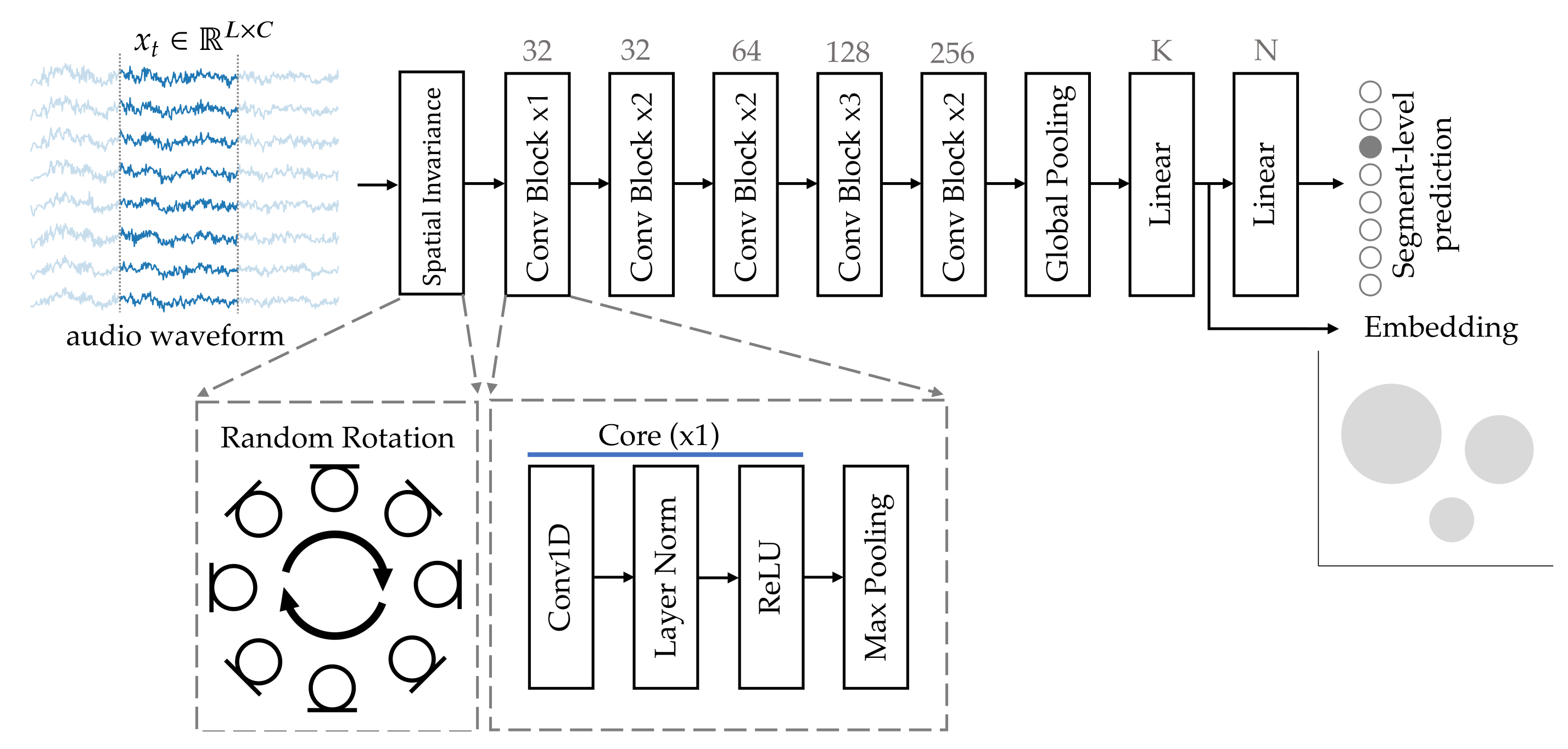
  • We demonstrate the effectiveness of one-dimensional deep convolutional neural networks to learn useful descriptions of real-world machine equipment from their emitted sound by processing raw audio directly;
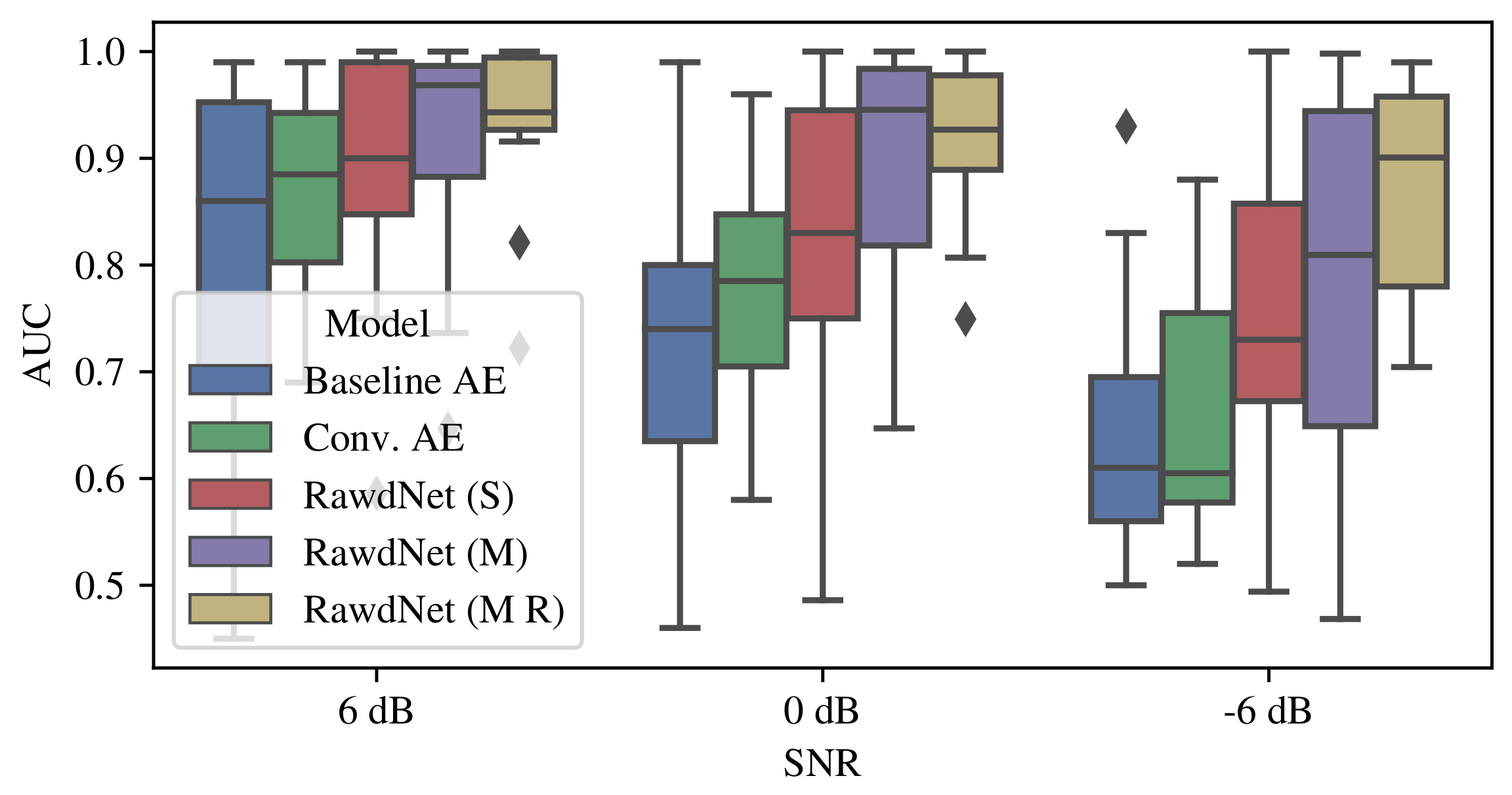
  • We explore the use of multi-channel audio recordings to exploit spatial audio information and propose a naive front-end training strategy that enables the network to effectively learn spatial and spectro-temporal audio features;
  • We show that by jointly supervising a latent state of the deep convolutional neural network and the corresponding classification output, the model elicits highly discriminative features. This approach is applicable to a wide range of audio recognition tasks in the context of transfer learning.

2. Related Work

Recently, numerous novel machine condition monitoring techniques using vibration and acoustic emission signals have been researched for diverse industrial applications [18,23]. Signal analysis methods have been proposed to detect, identify, and diagnose faults in diesel engines [24], induction motors [25,26], rotating machinery [27], gearboxes [28,29], centrifugal pumps [30], and other mechanical equipment.
In most of the above research, a feature extraction stage is first employed to capture the most important temporal, spectral, and cepstral signal properties in a low-dimensionality space [31]. Mainly, these features are selected to reflect the particular conditions of the equipment, imposing the framework to be either machine-specific or machine type-specific [32]. Although this approach reconciles the system performance and interpretability, it lacks generalizability and hinders further practical applications. Thus, there is a shortage of data-driven condition monitoring methods in recent literature that can be considered general, in the sense that they can be applied to a wide scope of machinery with no or minimal modifications.
Second, a decision module is employed to detect out-of-distribution samples, which can be regarded as a one-class classifier [33,34]. Studies with one or an ensemble of support vector machines (SVMs) have been recently conducted in attempts to model the distribution of machine operating conditions for fault assessment and condition monitoring [35]. However, these methods are limited due to the SVM’s sensitive hyper-parameters and susceptibility to noise.
With the surge in deep learning and semantic audio analysis [36,37,38], recent studies have focused on the fault detection task through machine operating sounds using neural networks [12,39,40]. Recently, ref. [39] employed a neural network with an autoencoder structure to detect abnormalities in the emitted sound of a surface-mount device. Moreover, ref. [40] proposed an objective function based on the Neyman–Pearson lemma to train an autoencoder, formulating the AD task as a statistical hypothesis test. [12] provided an ensemble of convolutional autoencoders for audio-driven anomaly detection, which follows a cross-mapping strategy between different parts of the frequency spectrum. In the above approaches, the autoencoders are trained to reconstruct regular samples by learning an efficient representation of the input vector. Then, the model reconstruction residual-error is used as a similarity metric to detect machine malfunctions. In these approaches, the role of time-frequency audio data pre-processing and feature extraction is a crucial factor for system performance and generalization [41].
A new method has recently been introduced for neural network-based anomaly detection: the deep support vector data description (Deep SVDD) [10,42]. In Deep SVDD, a neural network is trained to extract representations of the input data that satisfy a one-class classification objective. This can be interpreted as minimizing the volume of a hypersphere that encloses the training data feature representations [43]. This way, the network is forced to extract the common factors of variation since it must closely map the data points to a hypersphere.
In the field of similarity learning, the use of embeddings has been explored as a method to map objects into specific groups of similar properties and features [44,45]. Unlike clustering, this approach benefits from supervising both the embedding extraction stage and the cluster formation in a joint training framework. Hence, the training aims to extract salient features from the input data that support the formation of class-determined clusters based on their corresponding similarity [46]. Moreover, there is no need for employing a separate optimization algorithm for clustering, since the embedding extraction stage is part of the unified model structure and is efficiently trained through statistical gradient descent. Depending on the task, different similarity metrics can be exploited for adapting the clusters to an auxiliary target distribution [47].
A similarity function has been proposed by [48] to detect anomalous sounds using an attention-based feature extractor for measuring similarity in embedded space. The advantage of this approach is that it is robust against changes in time-frequency structure (i.e., absorbing time-frequency stretching in the normal-class modeling).

3. Materials and Methods

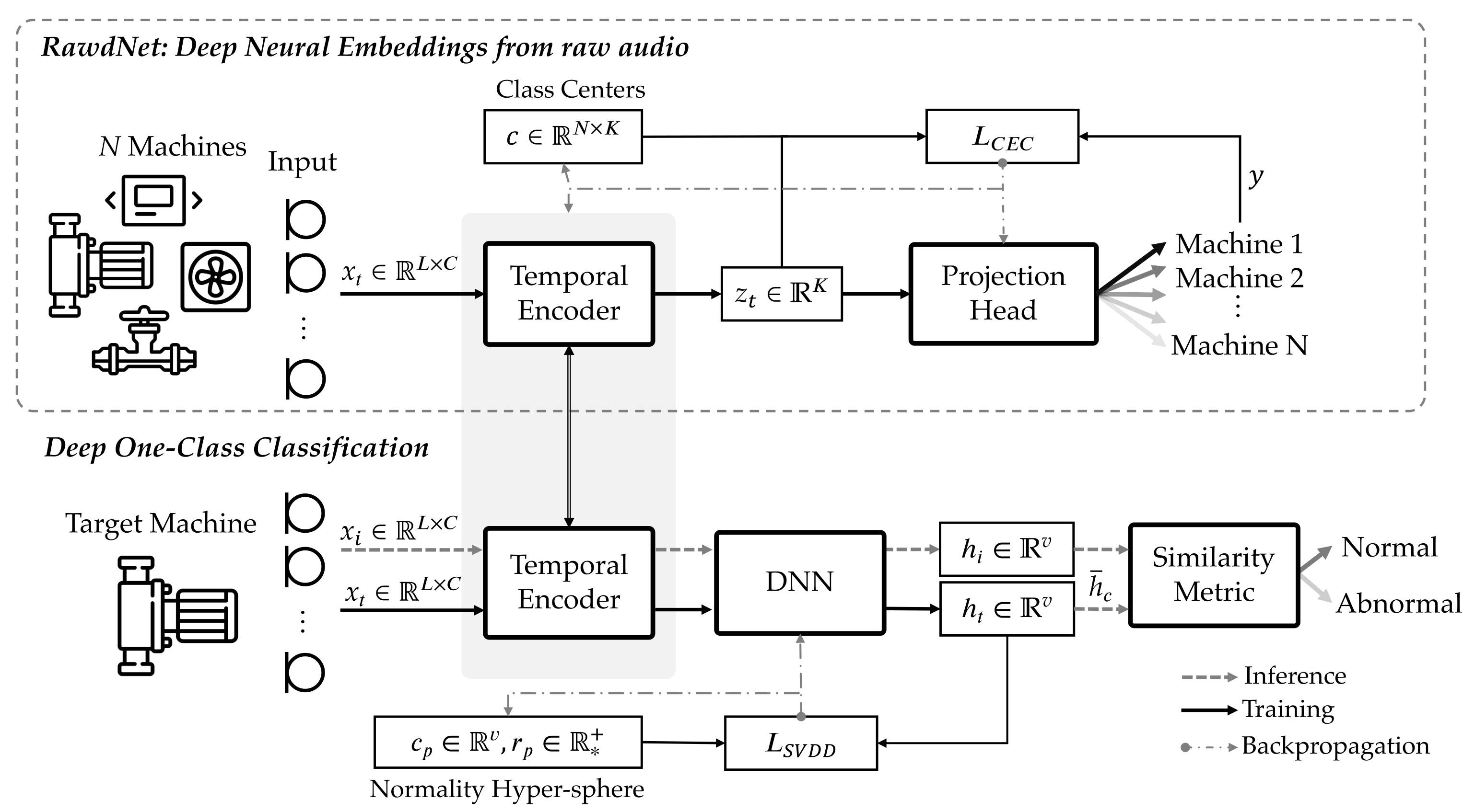
3.1. Overview and Motivation

Our approach to audio-driven anomaly detection can be divided into two stages: feature learning and class modeling. Instead of using a direct approach to anomaly detection, which is to model a one-class classifier on normal class samples, we introduce a two-stage method that provides the one-class classifier with dynamically extracted feature vectors. First, we aim to learn highly descriptive representations for a wide set of machine sounds in a classification framework. Second, we use this knowledge as a feature extraction stage to achieve concise normality modeling for each class. We propose a comprehensive learning approach that leverages information from other classes by enabling the formation of distinct clusters for each machine in an arbitrary low-dimensional space. Hence, the intermediate vector space should apparently be interpreted as a description of deviating examples, by enclosing the target anomalies.
The latter stage consists of class modeling for individual machines. The proposed one-class classifier consists of a deep neural network that takes as inputs the normal-class latent embeddings for a specific machine and maps them to an arbitrary low-dimensional vector space, so that the output distribution density is maximized. In this case, the Euclidean distance and cosine similarity can be effectively used as similarity metrics [49,50].
The proposed semi-supervised anomaly detection method can be graphically depicted in Figure 1. The following sections describe the data corpus used for the experiments, the proposed model architecture for learning discriminative embeddings from multichannel raw audio (RawdNet), and the deep one-class classifier based on the SVDD premise.

3.2. Discriminative Features from Multi-Channel Raw Audio

For a microphone array of C 2 microphones, we first split the audio signal x ( i ) of each microphone into non-overlapping segments of length L, as:
x t ( i ) = x ( i ) [ t L : ( t + 1 ) L ] , t Z , i = 1 , , C
where t is the time index and the operator x [ a : b ] selects the values of x between the indices a and b. Thus, the model input for each iteration consists of the tensor x t , as:
x t = { x t ( 1 ) , , x t ( C ) } T
The model processes the input tensor x t using a feed-forward architecture of convolutional blocks, as shown in Figure 2. The core of each convolutional block consists of a temporal convolutional layer (Conv1D), a normalization layer (Layer Norm), and the rectified linear unit (ReLU) activation function g ( x ) = m a x ( x , 0 ) [51]. In general, a temporal convolutional layer [52] is mathematically defined as below.
x = x * w c + b
where w c is a two-dimensional tensor with learnable parameters and * is the convolution operator. In our implementation, we set the bias term b R to zero, as it is negated by the following normalization layer. Then, a downsampling operation is performed through a max pooling layer [53]. The max-pooling operator passes forward the maximum activation over non-overlapping rectangular regions of size P = 4 :
x ( t / P ) = max 0 i P ( x [ t L + i ] )
where · is the ceiling operator. Depending on the depth of the network, convolutional blocks can comprise of more than one core units before the downsampling operation, to enable deeper training [54].
The final model consists of 5 convolutional blocks with a total of 10 convolutional layers with learnable parameters. In the proposed architecture, the five convolutional blocks include 32, 32, 64, 128, and 256 convolving kernels, respectively. The first convolutional layer includes kernels of size 81 with a stride of 4 samples. The rest convolutional layers share the same configuration, where small kernels sizes of 3 and unit striding are employed. Layer normalization [55] is a critical component of the RawdNet architecture, computing the normalization statistics separately for each channel.
Then, mean-pooling is applied to the output of the last convolutional block, followed by two linear layers with no activation function. Moreover, dropout with a probability of 0.2 is applied before each linear layer during training. At inference, the model output y t can be formally defined as:
y t = W y T z t + b y
z t = W z T 1 L 5 j = 1 L 5 f θ ( x t ) i j + b z , i = 1 , 2 , , K 5
where f θ : R L × C R K 5 × L 5 denotes the CNN temporal encoder function parameterized by θ , the length L of each segment corresponds to a 2 s audio clip, K 5 = 256 and L 5 = 31 denote the kernel and signal size at the output of the 5-th convolutional block. The matrices W z R K 5 × K , W y R K × N are the learnable weights and b z R K 5 , b y R N are the bias terms of the projection head layers, respectively.

3.2.1. Training Objective

In a supervised setting, we attempt to classify the training samples to their corresponding machine ID label. Samples are drawn only from normal operating conditions. Therefore, we mainly focus on the latent representation z to obtain the discriminative embeddings, while the model output y assigns the model outputs to the ground truth labels of the N machines. By obtaining the embeddings in a latent state of the network and not from the model output, the embedding dimensionality can be arbitrarily chosen based on the task complexity. A determinant factor of this architecture is to not incorporate non-linear activation functions, such as ReLU, between the latent representation and the model output. Namely, the model output y corresponds to a linear transformation of the embeddings z, which prevents from over-training the projection head and assists the learning of prominent features by the convolutional layers.
The training objective for a multi-class classification problem usually relies on minimizing the cross-entropy loss function for each class. When the training converges, both the model predictions and latent representations should be to the most separable. Both outputs are not discriminative enough to provide meaningful information for further processing, since significant intra-class variability in the Euclidean sense is present [56,57]. To remedy this, we focus on minimizing the intra-class distances of the model projection on semantic labels [58].
Center loss enables the model to form qualitative clusters of the target classes into a continuous vector representation, by penalizing the distances between the latent features and their corresponding class centers. The center loss function can be expressed as:
L C = 1 2 i = 1 m z ( i ) c y i 2 2
where c y i denotes the class prototype of the i-th sample (referred to as c in Figure 1), m denotes the length of the mini-batch, z i and x i denote the encoder and projection head outputs for the i-th sample, respectively. The standard cross-entropy objective function L C E with the SoftMax function is employed to supervise the model output y, as:
L C E = i = 1 m y i ˇ log e y i j e y j
where y i ˇ denotes the ground truth label for the i-th sample.
Cross-entropy loss and center loss can be used to jointly supervise the training process. The resulting loss function can be written as:
L C E C = L C E + λ · L C
where λ is a scalar used for balancing the two loss functions. The L C E C loss function considers both the intra-class compactness of the latent representation, which is encouraged by the center loss, and the inter-class separability, which is enforced by the cross-entropy term in the linear mapping of z. Hence, discriminative embeddings for each machine ID would be obtained.
The parameter λ is considered a network hyperparameter, which can be changed during training according to some schedule. For this task, we found that joint training with static and equal weighting of the class separability and intra-class compactness objectives ( λ = 1 ) results in faster convergence.
Ideally, c y i would represent the class centers of the training data. However, computing this quantity over the entire dataset would be computationally expensive. Thus, we randomly initialize c y i and update it in every batch using the stochastic gradient descent (SGD) optimization algorithm with respect to L C E C . Moreover, the model parameters and class centers are updated with different learning rates ( l r = 0.0001 , l c = 0.01 ) to achieve robustness to sample perturbation and address potential scalability problems [59].

3.2.2. Data Augmentation for Spatial Invariance

Circular microphone arrays are quite common for recording multichannel audio, as they encourage the exploitation of spatial information contained in complex acoustic environments [60]. Techniques, such as independent component analysis, adaptive filtering, and beamforming, have long demonstrated the power of spatially-aware systems in localizing sound sources [61,62] and detecting audio events [63]. However, the majority of spatial filtering techniques require knowledge of the recording setup and are usually based on statistical assumptions that are not always met in real-world conditions, especially when multiple sound sources are present. Considering this, we investigate the efficacy of both single-channel and multi-channel audio in providing useful embeddings for the task of anomaly detection, by selecting the appropriate number of input channels to the RawdNet model, as it was mentioned in Section 3.2.
Regarding the multi-channel approach, our concern lies on the static location of each machine in both the training and testing recording setups, as the system is not adaptively trained to exploit the spatial information of the acoustic scene. So, if the spatial distribution of sound sources is slightly altered at inference, possible degradations to the system performance could be faced, unveiling characteristics of spatial over-fitting.
To address this problem, we formulate a front-end processing strategy that offers spatial invariance in circular microphone arrays, to avoid over-fitting issues arising from the static location of sound sources. In detail, we apply a randomized rotation of the microphone array in the model input, implemented by the roll operator R as:
R : ( x 1 , x 2 , , x C ) ( x C , x 1 , , x C 1 )
So, the model input x t is transformed to x t , as:
x t = R a ( x t )
where a Z is a uniformly distributed random variable and R n + 1 = R R n . In such, we enable the learning of directionally-independent spatial features in the deep neural network by maintaining inter-channel correlations of a rotation permutation scheme and simulating the random rotation of the microphone array.

3.3. Deep One-Class Classification

The support vector data description [64] is a method proposed for one-class classification that is closely related to the OC-SVM approach. A hypersphere is calculated to enclose the given data samples and eventually to separate inliers from outliers. This objective can be used to train a neural network and be applied to the learned network representation, comprising the unsupervised Deep SVDD method, as described by [42]. That is, ϕ W : R K R v is a neural network mapping function with parameters W. The goal is to estimate the optimal parameters W so that (a) a hypersphere encloses the feature representation of the input data distribution assigned by ϕ and (b) minimize the volume of the hypersphere in the output space. At inference, the distance from the center of the hypersphere is employed as the anomaly score of a sample. Consequently, feature representations that lie outside the learned hypersphere are considered anomalous. Alternatively, various similarity metrics can be used to calculate soft anomaly scores.
The Deep SVDD objective function L S V D D is defined as:
L S V D D = r p 2 + λ v m i = 1 m m a x 0 , ϕ W ( z ( i ) ) c p 2 r p 2
where m denotes the length of the mini-batch, and the sensitivity trade-off between class representation volume and penalty of outliers is controlled by the hyper-parameter λ v R + * . The parameters c v R v and r v R + * are vectors that represent the normality center and radius, respectively.
Similarly to Section 3.2.1, we avoid computing the center and radius parameters over the whole dataset. Instead, c v and r v are randomly initialized and are jointly updated through SGD optimization in every mini-batch iteration, using a high and controllable learning rate ( l c = 0.5 ). Thus, the sensitivity of the anomaly detection classifier is determined by the upper bound of the fraction of training errors and the lower bound of the fraction of support vectors [65].
The deep one-class classification (DOC) neural network takes as input an aggregated feature vector, that concatenates the embedding feature representations y for a decision-level audio segment. In the case of the MIMII dataset [66], the decision-level segments have a duration of 10 s. Thus, the DOC input vector for the i-th sample is given by:
z ( i ) = t z t ( i ) , t = 0 , 2 , 4 , , 8
where ∥ denotes the concatenation operator. That is, z R 125 is the concatenated vector of the five 25-dimensional feature representations, each corresponding to the embeddings for a two-second segment.
The architecture comprises of four fully-connected layers with no bias term and the ReLU activation function after all but the last layer. The four layers consist of 63, 32, 32, and v = 16 neurons for the given input dimensionality. The DOC model was trained using the Adam optimizer with a learning rate l r = 0.001 on embedding batches of size m = 128 for all SNRs conditions (6, 0, −6) dB of a specific machine ID.

3.4. Experimental Setup
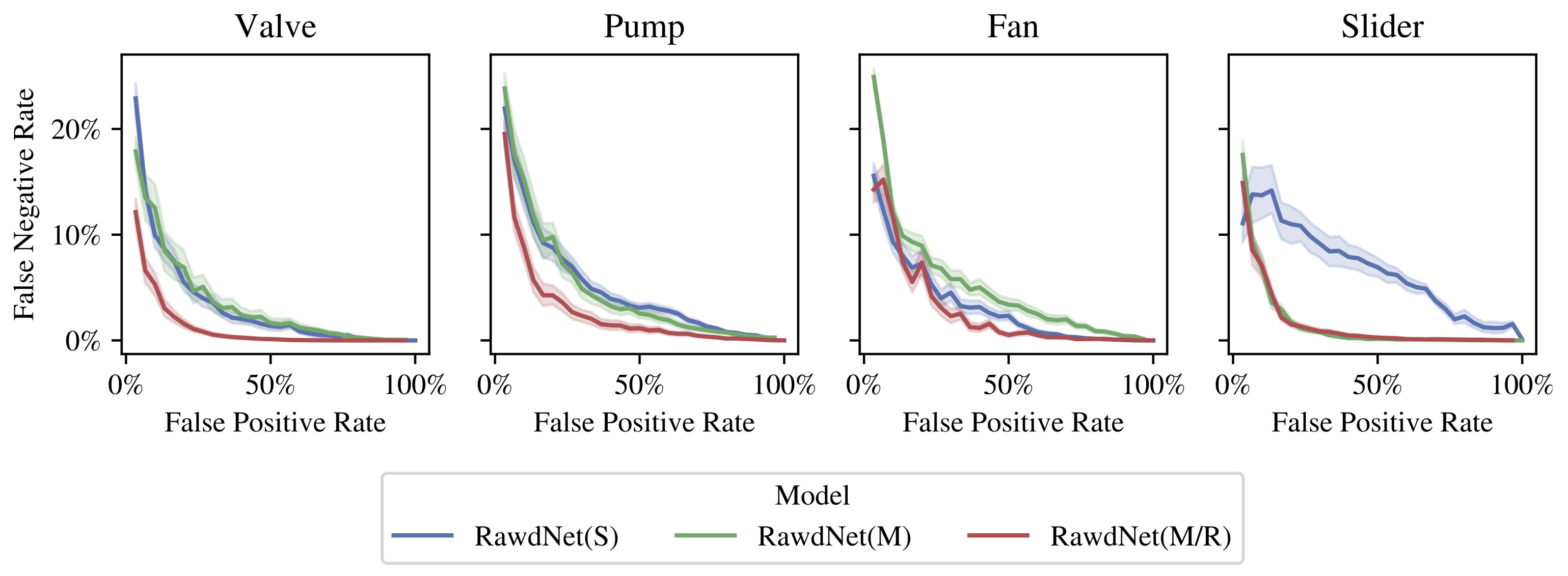
In this section, we describe the experiments conducted to evaluate the proposed approach and provide the essential details of the experimental setup. Experiments were conducted on the malfunctioning industrial machine inspection and investigation (MIMII) dataset [66]. The MIMII dataset includes multichannel recordings of twenty-eight industrial machines, which fall into four machine type categories (valve, pump, fan, slide rail). For each machine type, recordings of four individual machines (ID: 0, 2, 4, and 6) are available. Therefore, a single label is assigned to each audio segment depending on the condition of the machine, namely normal or abnormal. Recordings are mixed in variable signal-to-noise ratios (6, 0, and −6 dB) in simulated industrial environments and are provided in decision-level segments of 10 s. For a certain signal-to-noise ratio (SNR) γ dB, the noise-mixed data of each machine were created according to the following equation [66].
x ( i ) [ t ] = s ( i ) [ t ] + u ( i ) [ t ] · τ = 0 L s [ τ ] 2 τ = 0 L u [ τ ] 2 · 10 γ 10
where t is the time index, i is the channel index, and s and u are the clean target machine and background noise 10-s segments, respectively.
The sound recordings were obtained by a circular array of eight microphones ( C = 8 ); each sample contains eight separate channels for each audio segment. The recorded machines were spatially separated in the recording setup, making it useful for evaluating both single-channel and multi-channel-based approaches. In this study, we investigate the effectiveness of both single-channel and multi-channel approaches and propose a spatial invariance front-end for processing multi-channel raw audio using deep CNNs.
The MIMII dataset was split into training and test sets using stratified linear sampling (no shuffling). The development set, consisting of training and validation sets, includes the 70 % and 10 % of each machine ID normal data samples, respectively. The rest of the normal samples are used for testing along with all the abnormal samples of the dataset.
Effectiveness of RawdNet embeddings. To evaluate the proposed RawdNet model in extracting useful embeddings for the task of anomaly detection, a standard one-class SVM (OC-SVM) is employed along with the DOC classifier described in Section 3.3. Moreover, the OC-SVM model is used as a baseline to evaluate the performance of the proposed DOC and demonstrate the benefits of employing a neural network architecture as the back-end anomaly detector.
Effects of multi-channel audio. We consider the effectiveness of both single- and multi-channel approaches, to examine the potential of one-dimensional CNNs in extracting useful spatial features. For the single-channel approach, the first audio channel was employed as the model input, while for the multi-channel approach, all eight channels were employed.
Effects of the spatial invariance front-end. In Section 3.2.2, we propose to train the multi-channel RawdNet model on a front-end that aims to achieve spatial invariance. This is achieved by inter-changing the configuration of audio channels, simulating the rotation of circular arrays. Hence, the model performs the spatial filtering before extracting the latent embeddings, to reduce the dependence on a static microphone configuration.

4. Results

The proposed approach is objectively evaluated using the area under the receiver operating characteristics curve (AUC) metric on the soft anomaly scores of each classifier. The performance of the models is validated against two unsupervised anomaly detection models from recent works, which operate on the same dataset and configuration. The first is an autoencoder (AE) neural network model provided as a baseline model by the authors of the MIMII dataset [66]. The latter is a deep convolutional autoencoder (Conv. AE) with a dense-bottleneck structure from our previous work [12]. In an ablation study experiment, different configurations of the embedding extraction model (RawdNet) and one-class classifier (OC-SVM and DOC) are evaluated for their performance contribution, as described in Section 3.4.
The results for each machine type are shown in Table 1. Specifically, four individual machines with IDs of 0, 2, 4, 6 are given for each machine type (Valve, Pump, Fan, Slider). AUC values are averaged over the individual machines and are provided in a single value per SNR condition to deliberately demonstrate the robustness of each method.
The single-channel approach, denoted by RawdNet ( S ) , yielded improved (mean) AUC scores both using DOC (82.4%) and standard OCSVM (79.3%) back-end classifiers, compared to the autoencoder-based models (73.2% and 77.1%). Accordingly, significant improvements over all SNR conditions are observed for Valve (+25.4%) and Pump (+11.6%) machine types by the RawdNet(S)-DOC model over existing methods, while the indicated performance on Fan (+3.4%) and Slider (−3.6%) types are comparable to the unsupervised methods. Hence, the effectiveness of the proposed approach was demonstrated in this scenario, substantially improving the AD performance in cases where existing unsupervised deep learning methods struggle.
The multi-channel approach, denoted as RawdNet(M), demonstrated the potential of exploiting all available audio channels, noting a mean AUC increase of 4.3%. However, the mean AUC difference is mainly affected by the Slider class, where the multi-channel approach outperformed the RawdNet(S) model (+20.3%). The RawdNet(M) model achieved slightly lower performance than the single-channel model variant for Valve, Pump, and Fan machine types. Moreover, the control decision model (OC-SVM) achieved a slightly lower (78.8%) AD score than that of the single-channel approach.
It is worth noting that the model did not provide the expected performance increase for the amount of information supplied, indicating that it could not utilize the spatial properties of the audio signals. Another explanation is the emergence of potential over-fitting issues due to the higher input dimensionality. One possible explanation would be that the architecture of the CNN could be incapable of capturing the intended spatial features, inevitably leading to high input redundancy. To remedy this, we investigated a front-end input processing strategy based on the circular microphone array configuration used in the recording of the MIMII dataset.
The RawdNet(M/R) model consists of the same multi-channel encoder architecture that was trained on the spatial invariance front-end. This approach improved the performance of the latter model by 4.3% for the DOC approach, reaching a mean AUC score of 91.0%. Nevertheless, RawdNet(M/R) showed a 7.6% mean increase compared to the RawdNet(M) model and achieved significantly better performance than the other model variants in the majority of machine IDs, as shown in Figure 3. The model proved to be exceptionally robust to noisy environments, outperforming competitor models at −6 dB SNR (87.3%). Additionally, the effect of noise was less evident in the RawdNet(M/R) model performance, resulting in lower performance reduction and variance for different SNR conditions.
Class-dependent anomaly detection performance is illustrated in Figure 4, where different error types are considered. Parametric plotting of false negative rate (FNR) and false positive rate (FPR) are given by:
F P R ( τ ) = τ h 0 ( y ) d y
F N R ( τ ) = τ h 1 ( y ) d y
where h 0 and h 1 denote the genuine and impostor match score distributions of the anomaly class predictions, respectively. The spatial invariance front-end also contributes to lower error rates for valve, pump, and fan classes, while no significant contribution is observed between the RawdNet(M/R) and RawdNet(M) models for the slider class.
Furthermore, a comparison between the obtained results and those presented by [48] was conducted. [48] proposed a novel similarity function for AD (SPIDERnet) and validated it against three existing methods on a sub-set of the MIMII dataset, including three individual machines (Fan, Pump, Slider) at 0 dB SNR. The baseline methods include an autoencoder neural network (AE) as used by [40], a mean-squared error (MSE) similarity function that memorizes known anomalous functions [67], and a prototypical network-based (PROTOnet) AD framework [68]. According to the experiments, the SPIDERnet architecture achieved state-of-the-art AD performance. The authors employed the single-channel audio spectrogram coefficients as the input features to all models.
Table 2 shows that the proposed approach significantly outperforms all existing methods for the two out of the three tested machines. The AD performance in terms of the AUC metric is increased by up to 7 % and 5.3 % for the Pump (ID:06) and Slider (ID:02) machines, respectively. The proposed method did not perform comparatively for the Fan (ID:02) class. Although it provided better performance than AE and PROTOnet methods, SPIDERnet and MSE similarity functions achieved significantly better performance (+7.8% and +12.4%, respectively). These results are consistent with those of Table 1, in which the Conv. AE and AE models performed adequately on the Fan class at 0 and 6 dB SNRs, using a spectrogram representation as input features.
The effectiveness of RawdNet discriminative embeddings is demonstrated in Figure 5. In this experiment, we attempt to reduce the dimensionality of the embeddings and train the RawdNet model on the same data but with different objectives. It is apparent that the center loss term of the training objective imposes even the challenging two-dimensional embeddings of each class converge to the same point in the Euclidean sense and feature significant inter-class discriminability, compared to the SoftMax loss.
The enhanced performance of the model in most conditions can be possibly attributed to the extraction of more salient spatial features by the first convolutional layer. To demonstrate this, Figure 6 illustrates the spectral and spatial characteristics of the trained filters of the first convolutional layer, including the frequency and phase response of an exemplar multi-channel filter. Most of the thirty-two filters feature a narrow bandwidth to one or more spectral regions. The intra-kernel frequency deviations of multi-channel filters are rare or absent, in contrast to the deviations in the phase spectrum. Thus, it can be implied that the first convolutional layer is trained to exploit spatial information by emulating the responses of a multi-phase filterbank that aims to perform spectral and spatial analysis. For this reason, we attempt to visually interpret the spatial response patterns for the thirty-two filters of the first RawdNet(M/R) convolutional layer, by simulating the recording setup of the dataset by a sensor array of the same configuration [69]. The polar patterns of the initial layer show that a spatial filtering is performed in different patterns of directivity, corresponding to specific spectral regions.

5. Discussion

In this study, we emphasize the importance of temporal sound characteristics in the determination of a machine condition via deep learning. Experiments are conducted on a large real-world benchmark dataset, while each component of the proposed approach is exclusively evaluated in terms of its contribution to the overall AD performance. Visual insights on the proposed method are also provided, through the illustration of the spatial and spectral properties of the learned convolutional filters and the demonstration of exemplar cluster formation of the network’s embeddings.
We explicitly perform processing on raw audio by incorporating deep CNNs, which have recently demonstrated vast potential in modeling high-dimensional data. The learning of spatial audio features is also promoted by showing that multi-channel audio can be exploited to extract valuable spatial features, without the need of specifying the exact microphone configuration. Although this increases the data redundancy in the network, it also enables the search for particular short-duration temporal patterns of target sounds.
The architecture of the RawdNet model primarily consists of convolutional and downsampling layers, while no dropout strategy proved to assist better training. The use of layer normalization instead of batch normalization played a significant role in the model performance, drastically reducing over-fitting in the initial experiments. Layer normalization seems to better stabilize the input of each hidden convolutional layer compared to batch normalization and prevents learning under distribution shifts [70]. The embedding learning process employed cross-entropy combined with the recently-introduced center loss objective. In contrast to [58], we propose to use center loss in a latent state of the network. The combination of the two training objectives in different network states is a vital step in obtaining compact and discriminative embeddings along with stable training.
The experiments in Section 4 demonstrate that the proposed two-stage approach enables the accurate detection of unknown anomalies and is robust under adverse noise conditions. Previous research on this field mainly employed the mel-scaled or linear spectrogram coefficients as input features for deep learning-based anomaly detection [7,39,48,67,71,72]. Here, the enhanced performance in most conditions can possibly be attributed to the extraction of more salient spatial and spectro-temporal features by the one-dimensional CNN.
The superiority of the proposed architecture for detecting faults in Valve and Slider machine types indicates that one-dimensional CNNs are capable of capturing particular short-duration temporal patterns of target sounds. The performance gain is less evident or absent in cases where spectral patterns are more important for detecting anomalies (temporal modulation patterns are absent or not relevant) and high SNR conditions are expected at inference. In these cases (e.g., Fan, Pump), the AD task is better addressed by spectral analysis.
One limitation of the proposed method is that to perform the normality modeling for a novel machine, the model must be trained with all the available data, which leads to a time-consuming training process. This can potentially be addressed by training a large model on a dataset with numerous classes and assess the performance in the AD task for a new machine without retraining. In addition, since the two stages of the proposed approach are independent, the AD performance cannot be easily monitored during the training of the RawdNet model. Practically, this implies that the reduction in the proposed loss in the RawdNet model does not necessarily lead to a direct performance increase.
Future studies on audio-driven AD should explore the potential of end-to-end models for semi-supervised AD, as well as the unsupervised discrimination between different conditions of a machine in clustering-free approaches. Furthermore, adaptive front-ends and trainable spatial filtering methods for deep learning-based audio recognition should be further investigated.

6. Conclusions

In this study, we investigate the extraction of discriminative embeddings for a wide set of machinery sounds from multi-channel raw audio. Machine embeddings are learned by a deep convolutional neural network and are transferred to a deep one-class neural network to detect faults on individual machines. Experimental results show that the proposed approach can consistently model the normal conditions of various machines and accurately detect system faults. The proposed RawdNet model outperforms state-of-the-art audio-driven fault detection methods in most tested cases and is significantly more robust in noisy environments. Additionally, one-dimensional convolutional neural networks proved capable of extracting valuable spatial and spectro-temporal information from multi-channel audio, which had the effect of substantially improving the robustness of the latent discriminative embeddings. Finally, the proposed training objective of the two neural networks can account for the solid performance of a one-class classifier, by jointly maximizing the similarity and density of the normal data distribution.

Author Contributions

I.T.: Conceptualization, Methodology, Formal Analysis, Writing—Original draft preparation. M.G.: Data curation, Investigation, Writing—Reviewing and Editing. G.P.: Supervision, Conceptualization, Validation, Funding acquisition, Project administration. All authors have read and agreed to the published version of the manuscript.

Funding

This research is co-financed by Greece and the European Union (European Social Fund- ESF) through the Operational Programme “Human Resources Development, Education and Lifelong Learning 2014–2020” in the context of the project “Automated fault detection of industrial equipment based on audio analysis” (5047780).

Data Availability Statement

The code for reproducing the experiments and the detailed experimental results are available at a dedicated online repository https://github.com/jthois/semi-supervised-audio-based-machine-condition-monitoring (accessed on 30 September 2021).

Acknowledgments

We would like to thank Lazaros Vrysis for his collaboration in the conceptualization and implementation of the spatial invariance module.

Conflicts of Interest

The authors declare no conflict of interest.

Abbreviations

The following abbreviations are used in this manuscript:
Anomaly detectionAD
Condition monitoringCM
Convolutional neural networkCNN
Support vector machineSVMs
Support vector data descriptionSVDD

References

  1. Singh, G.K. Induction machine drive condition monitoring and diagnostic research—A survey. Electr. Power Syst. Res. 2003, 64, 145–158. [Google Scholar] [CrossRef]
  2. Hamamoto, A.H.; Carvalho, L.F.; Sampaio, L.D.H.; Abrão, T.; Proença, M.L., Jr. Network anomaly detection system using genetic algorithm and fuzzy logic. Expert Syst. Appl. 2018, 92, 390–402. [Google Scholar] [CrossRef]
  3. Liu, J.; Djurdjanovic, D.; Marko, K.A.; Ni, J. A divide and conquer approach to anomaly detection, localization and diagnosis. Mech. Syst. Signal Process. 2009, 23, 2488–2499. [Google Scholar] [CrossRef]
  4. Purarjomandlangrudi, A.; Ghapanchi, A.H.; Esmalifalak, M. A data mining approach for fault diagnosis: An application of anomaly detection algorithm. Measurement 2014, 55, 343–352. [Google Scholar] [CrossRef]
  5. Henriquez, P.; Alonso, J.B.; Ferrer, M.A.; Travieso, C.M. Review of automatic fault diagnosis systems using audio and vibration signals. IEEE Trans. Syst. Man, Cybern. Syst. 2013, 44, 642–652. [Google Scholar] [CrossRef]
  6. Urbanek, J.; Barszcz, T.; Antoni, J. Integrated modulation intensity distribution as a practical tool for condition monitoring. Appl. Acoust. 2014, 77, 184–194. [Google Scholar] [CrossRef]
  7. Yadav, S.K.; Tyagi, K.; Shah, B.; Kalra, P.K. Audio signature-based condition monitoring of internal combustion engine using FFT and correlation approach. IEEE Trans. Instrum. Meas. 2010, 60, 1217–1226. [Google Scholar] [CrossRef]
  8. Serin, G.; Sener, B.; Ozbayoglu, A.M.; Unver, H.O. Review of tool condition monitoring in machining and opportunities for deep learning. Int. J. Adv. Manuf. Technol. 2020, 109, 953–974. [Google Scholar] [CrossRef]
  9. Coraddu, A.; Oneto, L.; Ilardi, D.; Stoumpos, S.; Theotokatos, G. Marine dual fuel engines monitoring in the wild through weakly supervised data analytics. Eng. Appl. Artif. Intell. 2021, 100, 104179. [Google Scholar] [CrossRef]
  10. Ruff, L.; Vandermeulen, R.A.; Gornitz, N.; Binder, A.; Muller, E.; Kloft, M. Deep support vector data description for unsupervised and semi-supervised anomaly detection. In Proceedings of the ICML 2019 Workshop on Uncertainty and Robustness in Deep Learning, Long Beach, CA, USA, 14–15 June 2019; pp. 9–15. [Google Scholar]
  11. Davy, M.; Desobry, F.; Gretton, A.; Doncarli, C. An online support vector machine for abnormal events detection. Signal Process. 2006, 86, 2009–2025. [Google Scholar] [CrossRef]
  12. Thoidis, I.; Giouvanakis, M.; Papanikolaou, G. Audio-based detection of malfunctioning machines using deep convolutional autoencoders. In Audio Engineering Society Convention 148; Audio Engineering Society: New York, NY, USA, 2020. [Google Scholar]
  13. Vrysis, L.; Tsipas, N.; Dimoulas, C.; Papanikolaou, G. Crowdsourcing audio semantics by means of hybrid bimodal segmentation with hierarchical classification. J. Audio Eng. Soc. 2016, 64, 1042–1054. [Google Scholar] [CrossRef]
  14. Görnitz, N.; Kloft, M.; Rieck, K.; Brefeld, U. Toward supervised anomaly detection. J. Artif. Intell. Res. 2013, 46, 235–262. [Google Scholar] [CrossRef]
  15. Zhang, M.; Wu, J.; Lin, H.; Yuan, P.; Song, Y. The application of one-class classifier based on CNN in image defect detection. Procedia Comput. Sci. 2017, 114, 341–348. [Google Scholar] [CrossRef]
  16. Chandola, V.; Banerjee, A.; Kumar, V. Anomaly detection: A survey. ACM Comput. Surv. 2009, 41, 1–58. [Google Scholar] [CrossRef]
  17. Noto, K.; Brodley, C.; Slonim, D. FRaC: A feature-modeling approach for semi-supervised and unsupervised anomaly detection. Data Min. Knowl. Discov. 2012, 25, 109–133. [Google Scholar] [CrossRef] [PubMed] [Green Version]
  18. He, Q.; Yan, R.; Kong, F.; Du, R. Machine condition monitoring using principal component representations. Mech. Syst. Signal Process. 2009, 23, 446–466. [Google Scholar] [CrossRef]
  19. Diaz-Rozo, J.; Bielza, C.; Larrañaga, P. Machine-tool condition monitoring with Gaussian mixture models-based dynamic probabilistic clustering. Eng. Appl. Artif. Intell. 2020, 89, 103434. [Google Scholar] [CrossRef]
  20. Borghesi, A.; Bartolini, A.; Lombardi, M.; Milano, M.; Benini, L. A semisupervised autoencoder-based approach for anomaly detection in high performance computing systems. Eng. Appl. Artif. Intell. 2019, 85, 634–644. [Google Scholar] [CrossRef]
  21. Sarmadi, H.; Karamodin, A. A novel anomaly detection method based on adaptive Mahalanobis-squared distance and one-class kNN rule for structural health monitoring under environmental effects. Mech. Syst. Signal Process. 2020, 140, 106495. [Google Scholar] [CrossRef]
  22. De Benito-Gorron, D.; Lozano-Diez, A.; Toledano, D.T.; Gonzalez-Rodriguez, J. Exploring convolutional, recurrent, and hybrid deep neural networks for speech and music detection in a large audio dataset. EURASIP J. Audio Speech Music Process. 2019, 2019, 1–18. [Google Scholar] [CrossRef] [Green Version]
  23. Poveda-Martínez, P.; Ramis-Soriano, J. A comparison between psychoacoustic parameters and condition indicators for machinery fault diagnosis using vibration signals. Appl. Acoust. 2020, 166, 1–13. [Google Scholar] [CrossRef]
  24. Li, W.; Parkin, R.M.; Coy, J.; Gu, F. Acoustic based condition monitoring of a diesel engine using self-organising map networks. Appl. Acoust. 2002, 63, 699–711. [Google Scholar] [CrossRef]
  25. He, W.; Zi, Y.; Chen, B.; Wu, F.; He, Z. Automatic fault feature extraction of mechanical anomaly on induction motor bearing using ensemble super-wavelet transform. Mechan. Syst. Signal Process. 2015, 54–55, 457–480. [Google Scholar] [CrossRef]
  26. Glowacz, A. Acoustic based fault diagnosis of three-phase induction motor. Appl. Acoust. 2018, 137, 82–89. [Google Scholar] [CrossRef]
  27. Zhou, F.; Han, J.; Yang, X. Multivariate hierarchical multiscale fluctuation dispersion entropy: Applications to fault diagnosis of rotating machinery. Appl. Acoust. 2021, 182, 108271. [Google Scholar] [CrossRef]
  28. Yao, J.; Liu, C.; Song, K.; Feng, C.; Jiang, D. Fault diagnosis of planetary gearbox based on acoustic signals. Appl. Acoust. 2021, 181, 108151. [Google Scholar] [CrossRef]
  29. Loutas, T.H.; Sotiriades, G.; Kalaitzoglou, I.; Kostopoulos, V. Condition monitoring of a single-stage gearbox with artificially induced gear cracks utilizing on-line vibration and acoustic emission measurements. Appl. Acoust. 2009, 70, 1148–1159. [Google Scholar] [CrossRef]
  30. Kumar, A.; Gandhi, C.P.; Zhou, Y.; Kumar, R.; Xiang, J. Improved deep convolution neural network (CNN) for the identification of defects in the centrifugal pump using acoustic images. Appl. Acoust. 2020, 167, 107399. [Google Scholar] [CrossRef]
  31. Xia, S.; Zhang, J.; Ye, S.; Xu, B.; Xiang, J.; Tang, H. A mechanical fault detection strategy based on the doubly iterative empirical mode decomposition. Appl. Acoust. 2019, 155, 346–357. [Google Scholar] [CrossRef]
  32. Gowid, S.; Dixon, R.; Ghani, S. A novel robust automated FFT-based segmentation and features selection algorithm for acoustic emission condition based monitoring systems. Appl. Acoust. 2015, 88, 66–74. [Google Scholar] [CrossRef]
  33. Li, Z.; Li, J.; Wang, Y.; Wang, K. A deep learning approach for anomaly detection based on SAE and LSTM in mechanical equipment. Int. J. Adv. Manuf. Technol. 2019, 103, 499–510. [Google Scholar] [CrossRef]
  34. Potočnik, P.; Olmos, B.; Vodopivec, L.; Susič, E.; Govekar, E. Condition classification of heating systems valves based on acoustic features and machine learning. Appl. Acoust. 2021, 174, 107736. [Google Scholar] [CrossRef]
  35. Amarnath, M. Local fault assessment in a helical geared system via sound and vibration parameters using multiclass SVM Classifiers. Arch. Acoust. 2016, 41, 559–571. [Google Scholar] [CrossRef] [Green Version]
  36. Vryzas, N.; Vrysis, L.; Matsiola, M.; Kotsakis, R.; Dimoulas, C.; Kalliris, G. Continuous Speech Emotion Recognition with Convolutional Neural Networks. J. Audio Eng. Soc. 2020, 68, 14–24. [Google Scholar] [CrossRef]
  37. Amiriparian, S.; Gerczuk, M.; Ottl, S.; Stappen, L.; Baird, A.; Koebe, L.; Schuller, B. Towards cross-modal pre-training and learning tempo-spatial characteristics for audio recognition with convolutional and recurrent neural networks. EURASIP J. Audio Speech Music Process. 2020, 2020, 19. [Google Scholar] [CrossRef]
  38. Vrysis, L.; Tsipas, N.; Thoidis, I.; Dimoulas, C. 1D/2D Deep CNNs vs. Temporal Feature Integration for General Audio Classification. J. Audio Eng. Soc. 2020, 68, 66–77. [Google Scholar] [CrossRef]
  39. Oh, D.Y.; Yun, I.D. Residual error based anomaly detection using auto-encoder in SMD machine sound. Sensors 2018, 18, 1308. [Google Scholar] [CrossRef] [Green Version]
  40. Koizumi, Y.; Saito, S.; Uematsu, H.; Kawachi, Y.; Harada, N. Unsupervised Detection of Anomalous Sound Based on Deep Learning and the Neyman-Pearson Lemma. IEEE/ACM Trans. Audio Speech Lang. Process. 2019, 27, 212–224. [Google Scholar] [CrossRef] [Green Version]
  41. Vrysis, L.; Tsipas, N.; Dimoulas, C.; Papanikolaou, G. Extending Temporal Feature Integration for Semantic Audio Analysis. In Audio Engineering Society Convention 142; Audio Engineering Society: New York, NY, USA, 2017. [Google Scholar]
  42. Ruff, L.; Vandermeulen, R.; Goernitz, N.; Deecke, L.; Siddiqui, S.A.; Binder, A.; Müller, E.; Kloft, M. Deep one-class classification. In Proceedings of the International Conference on Machine Learning, Stockholm, Sweden, 10–15 July 2018; pp. 4393–4402. [Google Scholar]
  43. Zgarni, S.; Keskes, H.; Braham, A. Nested SVDD in DAG SVM for induction motor condition monitoring. Eng. Appl. Artif. Intell. 2018, 71, 210–215. [Google Scholar] [CrossRef]
  44. Xie, J.; Girshick, R.; Farhadi, A. Unsupervised deep embedding for clustering analysis. In Proceedings of the International Conference on Machine Learning, PMLR, New York, NY, USA, 19–24 June 2016; pp. 478–487. [Google Scholar]
  45. Olson, C.C.; Judd, K.P.; Nichols, J.M. Manifold learning techniques for unsupervised anomaly detection. Expert Syst. Appl. 2018, 91, 374–385. [Google Scholar] [CrossRef]
  46. Liu, Y.; He, L.; Liu, J.; Johnson, M.T. Introducing phonetic information to speaker embedding for speaker verification. EURASIP J. Audio Speech Music Process. 2019, 2019, 19. [Google Scholar] [CrossRef] [Green Version]
  47. Hershey, J.R.; Chen, Z.; Le Roux, J.; Watanabe, S. Deep clustering: Discriminative embeddings for segmentation and separation. In Proceedings of the 2016 IEEE International Conference on Acoustics, Speech and Signal Processing (ICASSP), Shanghai, China, 20–25 March 2016; pp. 31–35. [Google Scholar]
  48. Koizumi, Y.; Yasuda, M.; Murata, S.; Saito, S.; Uematsu, H.; Harada, N. Spidernet: Attention network for one-shot anomaly detection in sounds. In Proceedings of the ICASSP 2020—2020 IEEE International Conference on Acoustics, Speech and Signal Processing (ICASSP), Barcelona, Spain, 4–8 May 2020; pp. 281–285. [Google Scholar]
  49. Perera, P.; Patel, V.M. Learning deep features for one-class classification. IEEE Trans. Image Process. 2019, 28, 5450–5463. [Google Scholar] [CrossRef] [Green Version]
  50. Kwak, B.I.; Han, M.L.; Kim, H.K. Cosine similarity based anomaly detection methodology for the CAN bus. Expert Syst. Appl. 2021, 166, 114066. [Google Scholar] [CrossRef]
  51. Glorot, X.; Bordes, A.; Bengio, Y. Deep sparse rectifier neural networks. In Proceedings of the Fourteenth International Conference on Artificial Intelligence and Statistics, JMLR Workshop and Conference Proceedings, Ft. Lauderdale, FL, USA, 11–13 April 2011; pp. 315–323. [Google Scholar]
  52. LeCun, Y.; Bengio, Y. Convolutional networks for images, speech, and time series. Handb. Brain Theory Neural Netw. 1995, 3361, 1995. [Google Scholar]
  53. Ranzato, M.; Boureau, Y.L.; LeCun, Y. Sparse feature learning for deep belief networks. Adv. Neural Inf. Process. Syst. 2007, 20, 1185–1192. [Google Scholar]
  54. Vrysis, L.; Hadjileontiadis, L.; Thoidis, I.; Dimoulas, C.; Papanikolaou, G. Enhanced Temporal Feature Integration in Audio Semantics. J. Audio Eng. Soc. 2021, 68, 66–77. [Google Scholar] [CrossRef]
  55. Ba, J.L.; Kiros, J.R.; Hinton, G.E. Layer normalization. arXiv 2016, arXiv:1607.06450. [Google Scholar]
  56. Qi, C.; Su, F. Contrastive-center loss for deep neural networks. In Proceedings of the 2017 IEEE International Conference on Image Processing (ICIP), Beijing, China, 17–20 September 2017; pp. 2851–2855. [Google Scholar]
  57. Yang, J.; Xu, L.; Ren, B.; Ji, Y. Discriminative features based on modified log magnitude spectrum for playback speech detection. EURASIP J. Audio Speech Music Process. 2020, 2020, 1–14. [Google Scholar] [CrossRef]
  58. Wen, Y.; Zhang, K.; Li, Z.; Qiao, Y. A discriminative feature learning approach for deep face recognition. In Proceedings of the European Conference on Computer Vision, Amsterdam, The Netherlands, 11–14 October 2016; Springer: Berlin/Heidelberg, Germany, 2016; pp. 499–515. [Google Scholar]
  59. Li, N.; Tuo, D.; Su, D.; Li, Z.; Yu, D.; Tencent, A.; Deep Discriminative Embeddings for Duration Robust Speaker Verification. Interspeech. 2018, pp. 2262–2266. Available online: https://ai.tencent.com/ailab/media/publications/DeepDiscriminativeEmbeddingsforDurationRobustSpeakerVeri%EF%AC%81cation.pdf (accessed on 30 September 2021).
  60. Politis, A.; Vilkamo, J.; Pulkki, V. Sector-Based Parametric Sound Field Reproduction in the Spherical Harmonic Domain. IEEE J. Sel. Top. Signal Process. 2015, 9, 852–866. [Google Scholar] [CrossRef]
  61. Chen, J.C.; Yao, K.; Hudson, R.E. Source localization and beamforming. IEEE Signal Process. Mag. 2002, 19, 30–39. [Google Scholar] [CrossRef] [Green Version]
  62. Vryzas, N.; Dimoulas, C.A.; Papanikolaou, G.V. Embedding sound localization and spatial audio interaction through coincident microphones arrays. In Proceedings of the Audio Mostly 2015 on Interaction With Sound, Thessaloniki, Greece, 7–9 October 2015; pp. 1–8. [Google Scholar]
  63. Vryzas, N.; Kotsakis, R.; Dimoulas, C.A.; Kalliris, G. Investigating Multimodal Audiovisual Event Detection and Localization. In Proceedings of the Audio Mostly 2016, Norrkoping, Sweden, 4–6 October 2016; pp. 97–104. [Google Scholar]
  64. Tax, D.M.; Duin, R.P. Support Vector Data Description. Mach. Learn. 2004, 54, 45–66. [Google Scholar] [CrossRef] [Green Version]
  65. Liu, Y.; Madden, M.G. One-class support vector machine calibration using particle swarm optimisation. In Proceedings of the 18th Irish Conference on Artificial Intelligence, Dublin, Ireland, 29–31 August 2007; pp. 9–100. [Google Scholar]
  66. Purohit, H.; Tanabe, R.; Ichige, K.; Endo, T.; Nikaido, Y.; Suefusa, K.; Kawaguchi, Y. MIMII dataset: Sound dataset for malfunctioning industrial machine investigation and inspection. In Proceedings of the Acoustic Scenes and Events 2019 Workshop (DCASE2019), New York, NY, USA, 25–26 October 2019; p. 209. [Google Scholar]
  67. Koizumi, Y.; Murata, S.; Harada, N.; Saito, S.; Uematsu, H. SNIPER: Few-shot learning for anomaly detection to minimize false-negative rate with ensured true-positive rate. In Proceedings of the ICASSP 2019—2019 IEEE International Conference on Acoustics, Speech and Signal Processing (ICASSP), Brighton, UK, 12–17 May 2019; pp. 915–919. [Google Scholar]
  68. Pons, J.; Serrà, J.; Serra, X. Training neural audio classifiers with few data. In Proceedings of the ICASSP 2019—2019 IEEE International Conference on Acoustics, Speech and Signal Processing (ICASSP), Brighton, UK, 12–17 May 2019; pp. 16–20. [Google Scholar]
  69. Politis, A.; Laitinen, M.V.; Ahonen, J.; Pulkki, V. Parametric spatial audio processing of spaced microphone array recordings for multichannel reproduction. J. Audio Eng. Soc. 2015, 63, 216–227. [Google Scholar] [CrossRef]
  70. Vrysis, L.; Thoidis, I.; Dimoulas, C.; Papanikolaou, G. Experimenting with 1D CNN Architectures for Generic Audio Classification. In Audio Engineering Society Convention 148; Audio Engineering Society: New York, NY, USA, 2020. [Google Scholar]
  71. Chakrabarty, D.; Elhilali, M. Abnormal sound event detection using temporal trajectories mixtures. In Proceedings of the 2016 IEEE International Conference on Acoustics, Speech and Signal Processing (ICASSP), Shanghai, China, 20–25 March 2016; pp. 216–220. [Google Scholar]
  72. Thoidis, I.; Vrysis, L.; Pastiadis, K.; Markou, K.; Papanikolaou, G. Investigation of an Encoder-Decoder LSTM model on the enhancement of speech intelligibility in noise for hearing impaired listeners. In Proceedings of the AES 146th International Convention, Dublin, Ireland, 20–23 March 2019. [Google Scholar]
Figure 1. Schematic of the proposed system.
Electronics 10 02471 g001
Figure 2. Architecture of RawdNet.
Electronics 10 02471 g002
Figure 3. AUC (area under the curve) scores of the baseline and proposed models under various SNR (signal-to-noise ratio) conditions. AUC results are aggregated for all machine types and IDs.
Electronics 10 02471 g003
Figure 4. Detection error trade-off (DET) for the anomalous class. The performance of single-channel (S), multi-channel (M), and multi-channel with the spatial invariant front-end (M/R) RawdNet models is presented. The deep one-class classifier is selected as the decision module in all model variants. DET lines represent the average for all machine IDs (0, 2, 4, 6) and SNR conditions (−6, 0, and 6 dB) with shaded confidence interval 95%.
Electronics 10 02471 g004
Figure 5. Two-dimensional latent embeddings of the MIMII dataset produced by RawdNet ( K 5 = 2 ) with cross-entropy L C E loss (a) and the joint L C E C loss (b).
Electronics 10 02471 g005
Figure 6. Up: Frequency (left) and phase (right) responses of an exemplar kernel of the first convolutional layer of RawdNet(M). Although, the frequency response of the filters applied to each channel of the microphone array is quite similar, their phase response deviates significantly; Down: Normalized and logarithmically-scaled polar patterns for the 32 filters of the first convolutional layer. The polar responses were obtained by simulating the recording setup of the MIMII dataset.
Electronics 10 02471 g006
Table 1. Mean area under ROC curve scores for the anomaly detection on the MIMII dataset. Results are averaged for different machine types (IDs: 0, 2, 4, 6). The proposed single-channel (S) and multi-channel (M) convolutional neural embedding systems are combined with classical OC-SVM algorithm and DOC backend for anomaly detection. The incorporation of the spatial-invariance (R) front-end is denoted by the R indication.
MachineValvePumpFanSlider
SNR (dB)60−660−660−660−6
AE [66]67.061.355.580.570.566.091.382.068.887.878.070.0
Conv. AE [12]75.367.857.588.379.869.395.584.369.888.880.569.0
RawdNet(S)-OCSVM90.687.785.889.286.771.489.280.960.074.474.062.3
RawdNet(S)-DOC89.385.885.092.083.876.091.586.374.583.276.465.4
RawdNet(M)-OCSVM80.477.859.387.578.971.882.575.278.785.584.283.7
RawdNet(M)-DOC88.884.683.690.589.671.386.484.475.599.298.388.4
RawdNet(M/R)-OCSVM75.865.866.773.5 63.855.981.983.3 86.998.095.385.7
RawdNet(M/R)-DOC96.794.090.590.387.980.590.188.483.897.897.594.3
Table 2. AUC scores. Anomaly detection performance of the proposed method compared to those proposed by [48]. IDs 02, 06, and 02 of Fan, Pump, and Slider classes, respectively. All results correspond to the 0 dB SNR condition.
Machine (Type-ID) Fan-02 Pump-06Slider-02
Koizumi et al. [48]AE [40]52.840.385.9
MSE [67]91.243.894.7
PROTOnet [68]68.346.091.1
SPIDERnet95.888.092.5
OursRawdNet(S)-DOC75.090.079.0
RawdNet(M)-DOC83.495.094.1
RawdNet(M/R)-DOC 80.795.0100.0
Publisher’s Note: MDPI stays neutral with regard to jurisdictional claims in published maps and institutional affiliations.

