Experimental Analysis of Concentrated versus Distributed Massive MIMO in an Indoor Cell at 3.5 GHz

Abstract

This paper presents a measurement-based comparison between distributed and concentrated massive multiple-input multiple-output (MIMO) systems, which are called D-mMIMO and C-mMIMO systems, in an indoor environment considering a 400 MHz bandwidth centered at 3.5 GHz. In both cases, we have considered an array of 64 antennas in the base station and eight simultaneously active users. The work focuses on the characterization of both schemes in the up-link, considering the analysis of the sum capacity, the total spectral efficiency (SE) achievable by using the zero forcing (ZF) combining method, as well as the user fairness. The effect of the power imbalance between the different transmitters or user terminal (UT) locations, and thus, the benefits of performing an adequate power control are also investigated. The differences between the C-mMIMO and D-mMIMO channel performances are explained through the observation of the structure of their respective measured channel matrices through parameters such as the condition number or the power imbalance between the channels established by each UT. The channel measurements have been performed in the frequency domain, emulating a massive MIMO system in the framework of a time-domain duplex orthogonal frequency multiple access network (TDD-OFDM-MIMO). The characterization of the MIMO channel is based on the virtual array technique for both C-mMIMO and D-mMIMO systems. The deployment of the C-mMIMO and D-MIMO systems, as well as the distribution of users in the measurement environment, has been arranged as realistically as possible, avoiding the movement of people or machines.

1. Introduction

“Massive MIMO is a reality—What is next?” [1]. This suggestive paper presents various technologies based on the use of antenna arrays whose evolution will play an increasingly important role in the development of new generations of wireless communication systems (5G and beyond). Among them, the use of extremely large aperture arrays (ELAA) is presented as one of the most promising. Basically, the idea consists of distributing a great number of antennas over an extensive area, such as the roof of a big commercial building, or distributing them over a large geographical area, instead of grouping them into concentrated arrays, as has been the usual case so far. In this way, the user terminals (UTs) are surrounded by antennas belonging to a distributed base station (BS) instead of being covered by a BS with all its antennas concentrated in a classic array. The hybridization of proposals to evolve toward distributed wireless communication systems [2,3,4], together with the idea of massive multiple-input multiple-output (MIMO), has given rise to the concept of distributed massive MIMO [5,6,7,8,9,10] and the cell-free MIMO network concept [11,12,13,14].

Numerous theoretical works have investigated the performance of distributed massive MIMO (D-mMIMO) systems and their comparison with concentrated massive MIMO (C-mMIMO) systems. Obtaining adequate channel models is one of the difficulties in theoretical analysis of the capacity or spectral efficiency (SE) of distributed systems. Unlike concentrated systems, distributed ones present a great variability between the radio channels that a UT establishes with the different antennas conforming the BS. This is due to various propagation effects such as the path loss, shadowing effects, and degree of obstruction that each radio link experiences. This matter has been treated and modeled in the literature in different ways; see for instance [2,15,16,17,18].

Concerning experimental results, far fewer works can be found in the literature, all of them showing the advantages of the D-mMIMO system over the C-mMIMO one. In [19], an experimental analysis is carried out at 2.6 GHz; a C-mMIMO scheme is compared with another D-mMIMO one in the same indoor–outdoor environment and under non-line-of-sight (NLOS) conditions. It uses two arrays of 32 antennas that are placed together forming a concentrated 64 antenna element array, or two 32 antenna arrays 6.4 m apart, giving rise to a system which is, to a certain extent, distributed (split array). In summary, the conclusions are that the distributed configuration improves both the total throughput as well as the user fairness. In [20], an improved measurement system with regard to that presented in [19] is used in an indoor picocell. In this case, several antenna configurations are considered, where arrays consisting of 32 antennas are used, collocated, or distributed. In this case, the work is more focused on the proposal of new user scheduling algorithms than on the comparison of distributed versus collocated antenna configurations. In [21], an outdoor field experiment at 4.65 GHz of a distributed MIMO system is presented using sub-arrays of 2 × 2 antennas that are deployed on the terrace of a building in four positions 37 m apart. The total throughput is compared to that obtained with a concentrated MIMO system of 4 × 4 antennas. In both cases, eight UTs are considered moving at different speeds along the street surrounding the building. The main conclusion is that distributed MIMO has a better performance when compared with concentrated MIMO in cases of low mobility (5 km/h) and a similar performance in cases of high mobility (40 km/h). In [22], and using a similar experimental set-up as the one described in [21], a study is presented in the same frequency band, but now in an indoor environment. In this case, a significant increase in throughput is demonstrated when a distributed MIMO configuration is employed.

This paper presents a measurement-based comparison of distributed and concentrated massive MIMO systems, i.e., D-mMIMO and C-mMIMO systems, in an indoor environment. In both cases, we have considered an array of 64 antennas at the BS and eight simultaneously active UTs. The work focuses on the characterization of the channel in the up-link, considering the analysis of the capacity and the SE achievable by using the zero forcing (ZF) algorithm as the combining method, under the hypothesis of perfect channel state information (CSI). The effect of the power imbalance between the different UTs, and thus, the benefits of performing an adequate power control are also analyzed. In addition, user fairness is considered as another figure of merit in the comparison between both systems. Other important aspects related to the network architecture, such as the backhaul structure, the strategy to obtain CSI with minimal overhead, scheduling strategies, etc., remain outside the scope of this paper.

The channel measurements have been performed in the frequency domain, emulating a massive MIMO system in the framework of a time-domain duplex orthogonal frequency multiple access network (TDD-OFDM-MIMO). Moreover, the measurements have been carried out avoiding the movement of people in the building, considering a 400 MHz bandwidth centered at 3.5 GHz, with a frequency tone separation of 31.25 kHz, which is close to the 30 kHz established in the 5G standard numerology. The characterization of the MIMO channel is based on the virtual array technique for both C-mMIMO and D-mMIMO systems.

The main contributions of this paper are as follows: (i) The differences between the C-mMIMO and D-mMIMO channels are analyzed through the observation of the structure of their respective measured channel matrices, through parameters such as the condition number or the power imbalance between the channels established by each UT. (ii) The sum capacity of both types of channel is calculated and analyzed, and it is related to the structure of the channel matrix. (iii) Two alternative channel normalizations are used, one of which can be interpreted as the implementation by the system of an ideal power control. Thus, we quantify the impact of the power imbalance on the system performance and outline the advantages of carrying out an adequate power control. (iv) Beyond the intrinsic capacity of the channel, the achievable throughput is calculated using ZF as the combination method. (v) The latter allows us to analyze not only the total throughput achievable by each one of the schemes, distributed or concentrated, but also the user fairness that each of the methods offers, as a parameter of great interest when analyzing the pros and cons of both schemes.

The remainder of this paper is organized as follows. In Section 2, we present the channel characterization methodology for massive MIMO. Section 3 describes the indoor environment where the measurements are carried out along with the main characteristics of the channel sounders and the measurement settings. In Section 4, we present and analyze the results obtained from the experimental measurements. Finally, we conclude the paper in Section 5.

2. Channel Characterization Methodology

Focusing the analysis on the up-link, the massive MIMO system considered is a simple cell system where the BS is equipped with M antennas. The maximum number of active users is Q, and each UT is equipped with a single antenna. It is assumed that the users transmit a total power P. In addition, it is assumed that the BS knows the channel and that the UTs are not collaborating among each other. Furthermore, we consider an OFDM system with N_f sub-carriers, which correspond to the measured tones.

Considering this model, the vector form of the received signal at the BS for the k-th sub-carrier when the Q users are active will be given by:

$$y[k]=\sqrt{SNR}G[k]\cdot s[k]+n[k];k=1,2,\dots ,N_f,$$

(1)

where y[k] is a column vector with M elements corresponding to the k-th sub-carrier; G[k] is the channel matrix of order M × Q, in which each one of its columns corresponds with the narrowband channel of the q-th user g_q[k] of order M × 1; s[k] (Q × 1) is the vector representing the signals vector transmitted from the UTs and normalized in such a way that $E\left\{{\Vert s\Vert }^2\right\}=1$, where E{.} represents the mean or expected value; and n[k] is a complex Gaussian noise vector with independent and identically distributed (i.i.d.) unit variance elements. Finally, the SNR represents the mean signal to noise ratio at the receiver.

The matrix in (1) is normalized in such a way that verifies:

$$E\left\{{\Vert G\Vert }_F^2\right\}=M\cdot Q,$$

(2)

where ${\Vert .\Vert }_F$ is the Frobenius norm.

Moreover, the matrix G is obtained from the matrix of the raw channel measurements (G^raw) by means of:

$$G_{M\times Q}=G_{M\times Q}^{raw}{J}_{Q\times Q}.$$

(3)

The normalization matrix J is a diagonal matrix of order Q × Q. Different normalizations can be considered, provided they verify (2), which guarantees the conservation of the total transmitted power. Following the proposal and the nomenclature in [23], we consider two normalizations that we will denote as normalization 1 (N1) and normalization 2 (N2).

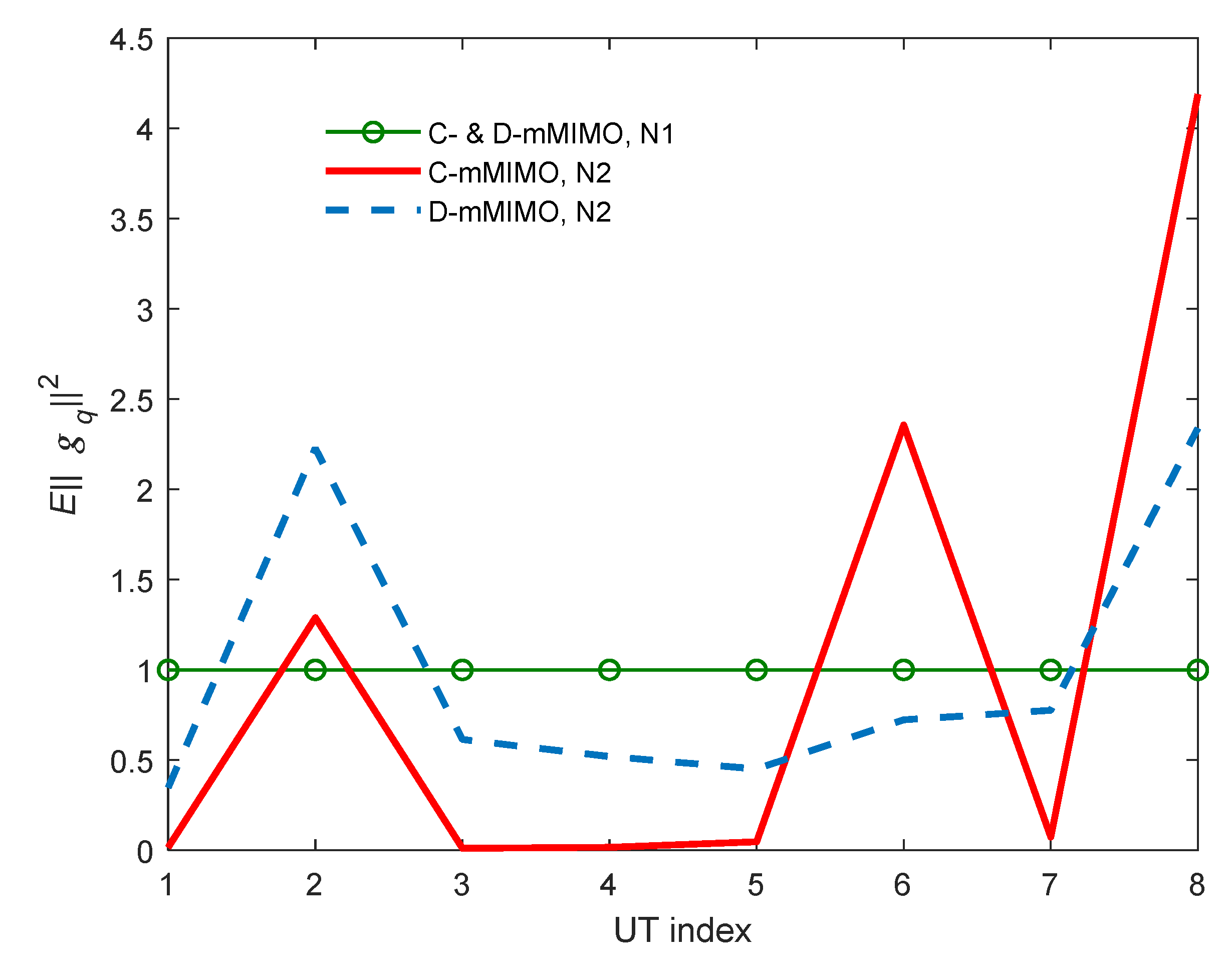
On the one hand, in case of using N1, the normalization matrix J is a diagonal matrix of order Q × Q, whose elements (j_qq) are given by

$$j_{qq}=\sqrt{\frac{M}{\frac{1}{N_f}{\displaystyle \sum _{k=1}^{N_f}{\Vert g_q^{raw}[k]\Vert }^2}}};q=1,\dots ,Q.$$

(4)

The elements of the normalization matrix J take different values so that all the columns in G are normalized to one; consequently, the power imbalance between the channels corresponding to each UT is eliminated, although the channel variations between antennas within the receiver array and frequency tones are maintained. The resulting normalized matrix, G, can be interpreted as that associated with a system in which an ideal power control is performed. In this case, the total available power transmitted by the users is not distributed equally, but each UT is assigned the necessary power so that all UTs reach the BS with the same mean power.

On the other hand, N2 is defined in such a way that all the elements of the diagonal matrix J are equal and thus, the operation in (3) is equivalent to multiplying the matrix by a scalar:

$$j_{qq}=\sqrt{\frac{MQ}{\frac{1}{N_f}{\displaystyle \sum _{k=1}^{N_f}{\Vert G^{raw}[k]\Vert }_F^2}}};q=1,\dots ,Q.$$

(5)

This normalization keeps the difference between the received power from different UTs, receiver antennas, and frequency tones.

Both N1 and N2 normalizations have their pros and cons. N2 preserves the original structure of the channel and the effect that the power imbalance can have on the system. However, if the aim is to isolate the effect of the power imbalance and exclusively analyze the orthogonality of the channel, for example through the condition number, it is mandatory to use N1 [23].

The SE that massive MIMO systems can achieve depends largely on the degree to which the condition of “favorable propagation” is met, which depends on the extent to which the channels of the different users are orthogonal [23,24,25,26,27]. A commonly accepted metric used to weigh up the orthogonality of the columns of a matrix is the condition number, κ, which is also a measure of the dispersion of the singular values of the matrix. The condition number of a matrix G is defined by the relationship:

$$\kappa =\frac{max\left\{eigenvalue(G^{H}G)\right\}}{min\left\{eigenvalue(G^{H}G)\right\}}.$$

(6)

According to (6), a value of κ equal to one corresponds to a channel matrix in which all its columns are orthogonal. Conversely, high values of κ indicate that at least two columns of the matrix will be practically collinear. It is more suitable to interpret the results to use the inverse of the condition number (ICN), which varies between 1 (maximum orthogonality) and 0 (zero orthogonality).

To have a direct measure of the goodness of the channel, we calculate the sum capacity. Under the hypothesis of a perfect knowledge of the channel at the BS, we can obtain the sum capacity of the massive MIMO-OFDM system by means of the breakdown into singular values of the channel matrix as

$$C\left[k\right]={\displaystyle \sum _{q=1}^Q{\log }_2\left(1+\frac{SNR}{Q}{\lambda }_q\left[k\right]\right);k=1,2,\dots ,N_f},$$

(7)

in which ${\lambda }_q$ represents the q-th eigenvalue of the G^HG matrix, i.e., the square of the q-th singular value of the G matrix.

Under favorable propagation conditions, as the number of receiving antennas M increases, and for a fixed number of transmitters Q, the capacity of the up-link channel will tend asymptotically to the upper bound [27]:

$$C_b=Q\cdot {\log }_2\left(1+\frac{M\cdot SNR}{Q}\right).$$

(8)

The sum capacity obtained from the concentrated system versus the distributed one allows a global comparison of the behavior of both systems to be made.

Furthermore, the analysis of the channel spectral efficiency provides additional information to compare both C-mMIMO and D-mMIMO systems. In this sense, both the individual SE for each user as well as the sum SE are calculated. Let us consider that the received signal is processed in the receiver by a linear combination method such as the ZF method, which is defined by the matrix V and expressed as

$$V=G{(G^{H}G)}^{-1}.$$

(9)

Then, the processed signal at the receiver can be expressed as

$$\widehat{s}\left[k\right]=V^H\left[k\right]y\left[k\right],$$

(10)

where $\widehat{s}$[k] is a column vector with Q elements that represents the estimation of the signals transmitted by the Q active users at the k-th frequency tone.

The signal to interference plus noise ratio (SINR) of the q-th user on the k-th sub-carrier is given by:

$$SIN{R}_q[k]=\frac{\frac{SNR}{Q}{\left|V_q^H{g}_q\right|}^2}{{\displaystyle \sum _{\begin{array}{l}i=1\\ i\ne q\end{array}}^Q\frac{SNR}{Q}{\left|V_q^H{g}_i\right|}^2+{\left|V_q\right|}^2}}.$$

(11)

Using (11), the individual SE of each active UT is calculated as follows:

$$S{E}_q[k]={\log }_2\left(1+SIN{R}_q[k]\right).$$

(12)

Finally, the sum SE is expressed as:

$$SE[k]={\displaystyle \sum _{q=1}^{Q}S{E}_q[k]}.$$

(13)

Another useful factor available to compare both C-mMIMO and D-mMIMO systems is the user fairness given by Jain’s Fairness Index (JFI) [28]. This metric is used to analyze the fairness of the channel to share out the overall SE among the active UTs, and it is given by:

$$JFI=E\left\{\frac{{\left({\displaystyle \sum _{q=1}^{Q}S{E}_q[k]}\right)}^2}{Q{\displaystyle \sum _{q=1}^{Q}S{E}_q^2[k]}}\right\},$$

(14)

where E{⋅} represents the mathematical expectation evaluated over all the N_f frequency tones. The JFI takes values between 1/Q and 1, so that the value 1 corresponds to the maximum fairness among the SE values of the active UTs.

3. Indoor Channel Measurements

In this section, the description of the indoor environment showing the distribution of both UTs and VAs for both situations (C-mMIMO and D-mMIMO), along with a summary including the main characteristics of the channel sounders and the measurement settings are presented.

In order to compare the experimentally obtained performance of both presented C-mMIMO and D-mMIMO configurations, a measurement campaign has been carried out inside a modern office building at the University of Cantabria. The measurements focus on the up-link and consider for the UTs both line-of-sight (LOS) as well as non-line-of-sight (NLOS) positions. Potential locations close to those that might be considered for a real deployment have been chosen for the virtual arrays (VAs) at the BS side. Regarding the channel sounding, we have considered two different measurement setups, both using a vector network analyzer as the main measurement equipment.

3.1. The Indoor Environment

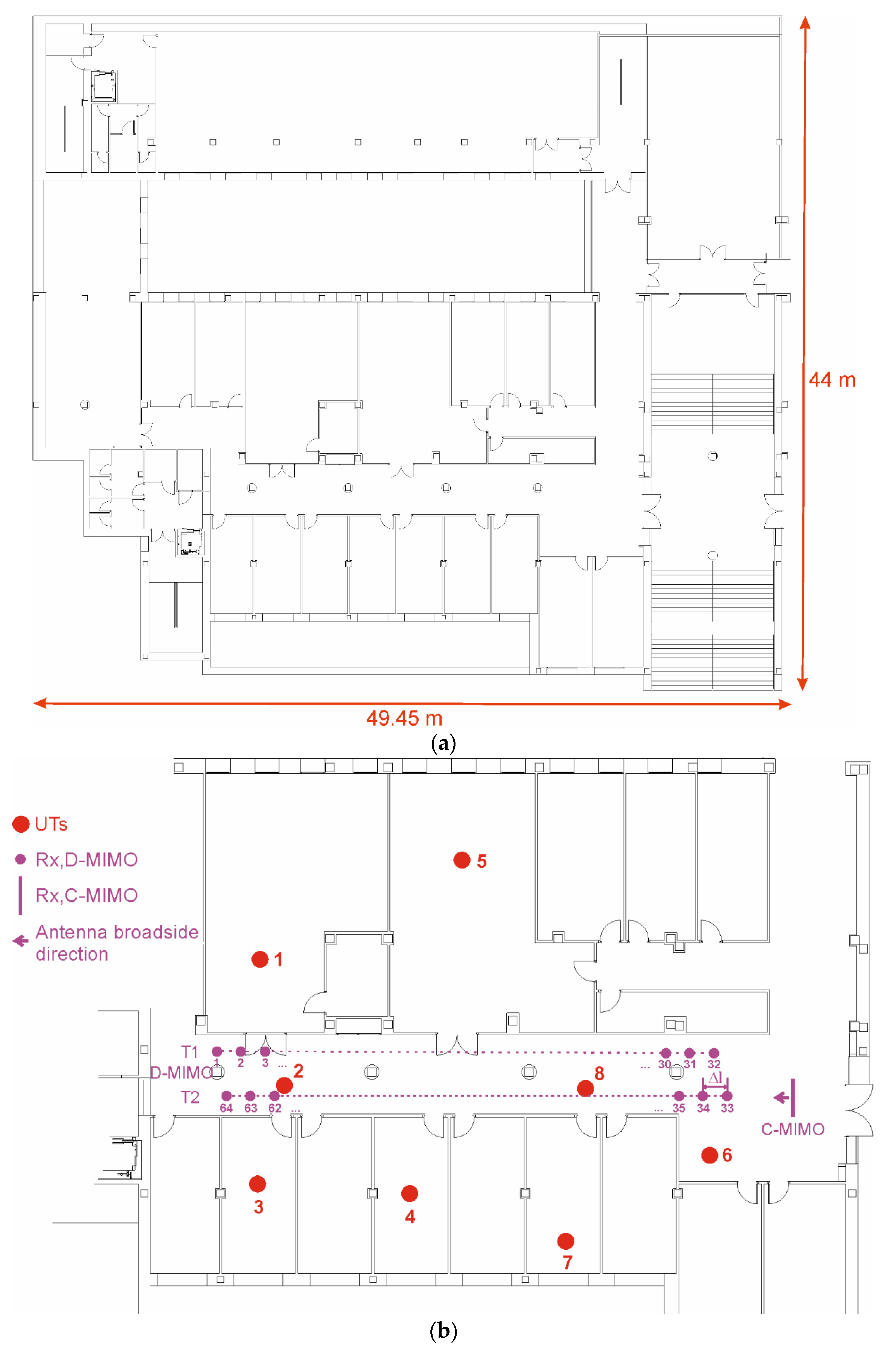
The top view of the indoor measurement environment considered in this work is shown in Figure 1a. The floor of the building mainly consists of offices and computer laboratories with a large corridor that provides access to those rooms. Regarding the materials of the building, it is made of reinforced concrete, has plasterboard paneled walls and ceiling boards, along with metallic doors in all the indoor rooms. The rooms are characterized by the presence of desks, chairs, and wooden and steel cabinets, along with computers and monitors.

According to the topology of the floor, the measurement campaign has concentrated on that part of the building shown in Figure 1b, including the details for both UTs and receiver (Rx) VA locations considered. It must be pointed out that there are four circular concrete columns almost centered in the corridor, which influence the multipath contributions reaching the Rx VAs and thus, the locations for such BS VAs must be carefully chosen. In this sense, the C-mMIMO VA consisting of 8 × 8 elements has been located near the main entrance of the building, at a height h_Rx for the center of the scanning area, and centered in the lower-widest half of the corridor. Furthermore, concerning the D-mMIMO VA arrangement, it consists of 64 antennas placed at the ceiling board at a height h_Rx, uniformly spaced Δl, and distributed over two linear trajectories, T1 and T2, which are located at both sides of the columns and linearly shifted from each other Δl/2.

Finally, eight potential UTs or transmitter (Tx) positions have been considered, mixing up two well-differentiated channel propagation conditions; some of them are under LOS conditions, i.e., UT₂, UT₆, and UT₈ (though strictly the UT₆ is under NLOS conditions for most of the D-mMIMO VA positions), and the rest are under NLOS conditions, i.e., UT₁, UTs_3-5, and UT₇. In this case, the Tx antenna is placed at a height h_Tx. The summary of the main parameters for both C-mMIMO and D-mMIMO virtual arrays, including those concerning the UTs, is presented in

Table 1. Parameters for the arrangement of concentrated massive multiple-input multiple-output (C-mMIMO), distributed massive multiple-input multiple-output (D-mMIMO), and user terminals (UTs).

C-mMIMO	VA size (y × z)	8 × 8
	VA inter-element separation at 3.5 GHz, Δy = Δz (mm/λ)	50/0.58
	VA total scanning area (m2)	0.1225
	Height at the center of the scanning area, hRx (m)	2.52
D-mMIMO	Number of antennas (T1 + T2)	64
	T1 and T2 inter-element separation at 3.5 GHz, Δl (mm/λ)	600/7
	Longitudinal shift between T1 and T2 (mm)	300
	Trajectory length, T1 = T2 (m)	18.60
	Height of the Rx antenna, hRx (m)	2.98
UTs	Height of the Tx antenna, hTx (m)	1.40

.

3.2. Measurement Setups

Two channel sounders have been used to carry out the measurements for both massive MIMO configurations. Basically, the two systems use a vector network analyzer (VNA) to measure in the frequency domain and in the frequency band of interest, i.e., 3.3–3.7 GHz, the S₂₁(f) scattering parameter that corresponds with the complex channel transfer function, H(f).

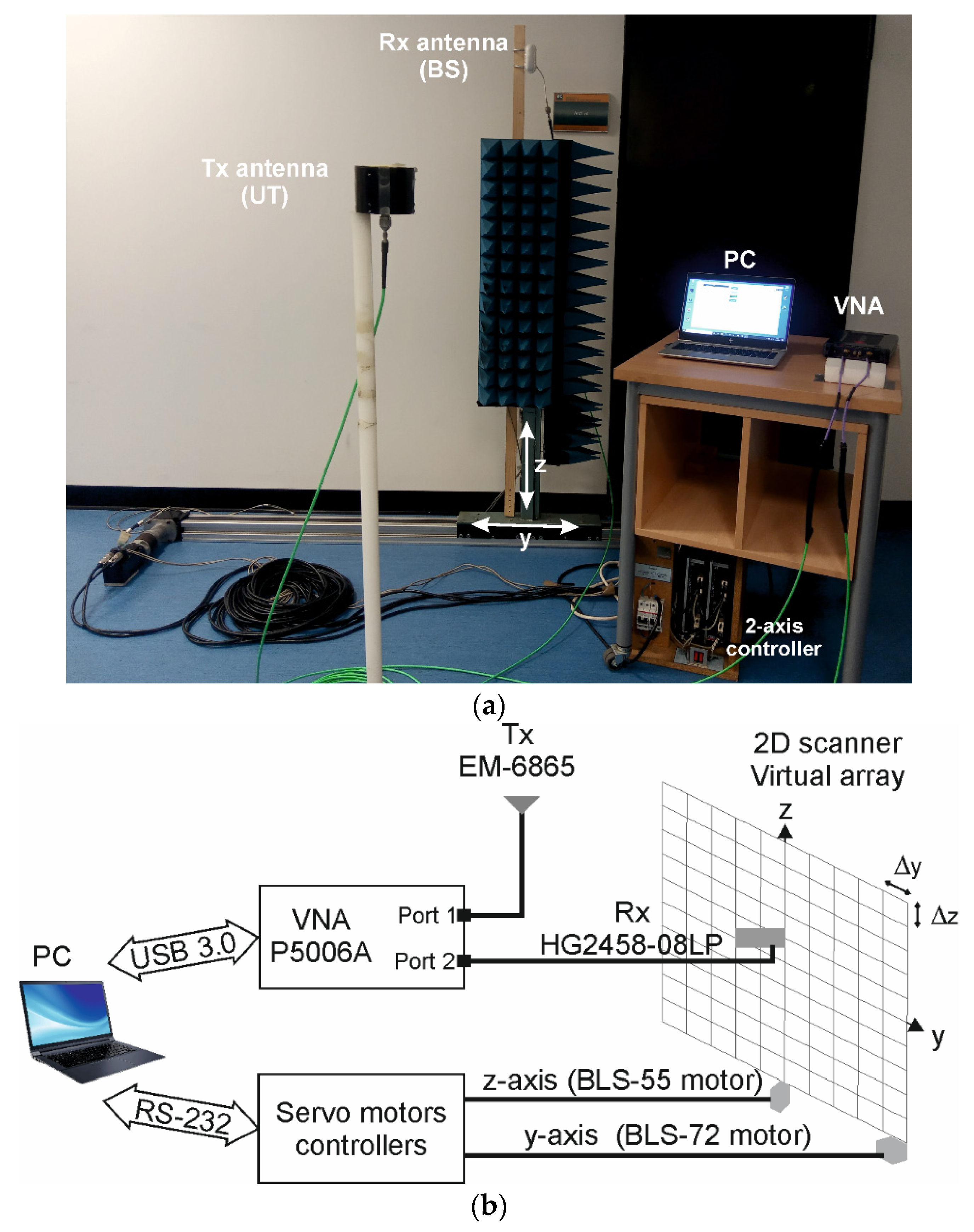
Concerning the C-mMIMO measurements, the automated measurement system used is shown in Figure 2. The channel sounder consists of a planar scanner and the P5006A VNA from Keysight Technologies, which are both remote controlled from a laptop to measure for a certain UT/Tx the H(f) at any Rx position of the VA over the YZ plane. The planar scanner consists of two linear units and the associated servomotors to control the movement in both axes, i.e., BLS-72 and BLS-55 motors from Mavilor. Compared with a previous channel sounder [29], the fitting of the speed of the motors and the use of the USB-controlled VNA speeds up the measurements significantly, the measurement for every UT position currently taking 20 min.

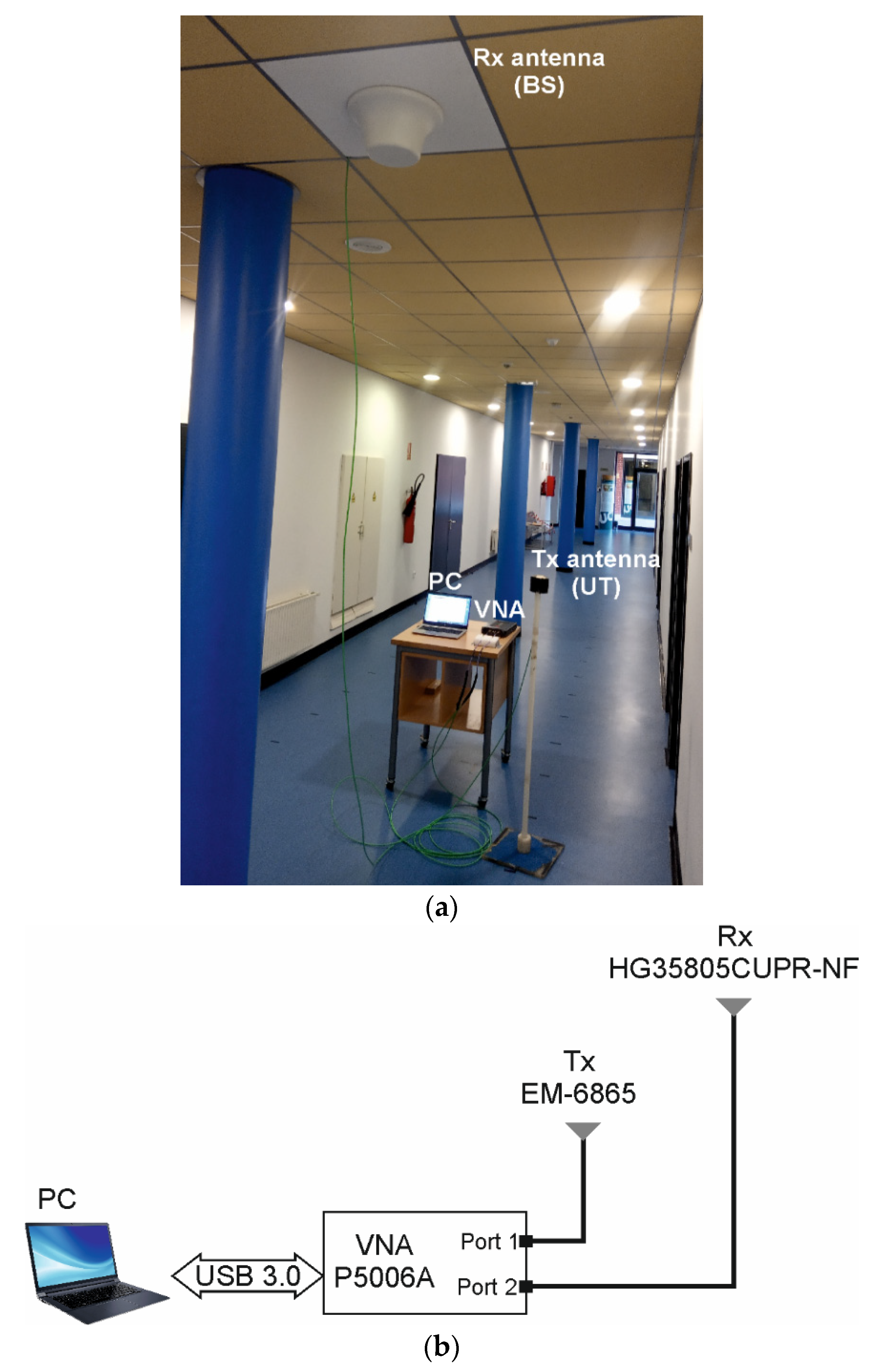
For the D-mMIMO measurements, we simplified the system used for the C-mMIMO setup by just eliminating the planar scanner. Basically, in this case and as shown in Figure 3, for every UT/Tx location, the Rx/Bs antenna is fixed to the ceiling board and manually moved to any of the 32 positions that make up both T1 and T2 trajectories. Bearing in mind again that the analysis is focused on the up-link, at every Rx position, the S₂₁-trace is acquired and, from the post-processing of the traces, a complete characterization of the indoor channel established between that Tx, i.e., an UT, and the Rx VA, i.e., the virtual array at the BS, can be carried out. Concerning the D-mMIMO measurement time, and in spite of the fact that the trace acquisition from the VNA takes less than 15 s per Rx position, the manual movement of the Rx antenna increases the overall measurement time for every UT position up to around one hour on average.

Regarding the antennas used in the measurement campaign, which are all linearly polarized, we have used the EM-6865 model from Electrometrics (a biconical omnidirectional antenna) on the Tx/UT side for both C-mMIMO and D-mMIMO measurements [29]. Furthermore, either the log-periodic HG2458-08LP [29] or the multi-band omnidirectional HG35805CUPR-NF antennas, both models from L-Com, have been used on the Rx/BS side for both C-mMIMO and D-mMIMO, respectively. Basically, the EM-6865 antenna operates in the 2–18 GHz frequency range and has a gain of around 1 dB in the band of interest, whereas the HG2458-08LP antenna operates in the 2.3–6.5 GHz frequency range showing a gain higher than 8 dBi and a beam width close to 60°. In [29], details for both antennas measured at 4 GHz are included. Moreover, the ceiling mount antennas, the HG35805CUPR-NF, show at 3.5 GHz a nearly omnidirectional pattern and a gain of 4.9 dB.

Finally, it must be pointed out that both sets of measurements, with the C-mMIMO and D-mMIMO systems, have been carried out at night to guarantee stationary conditions as the analysis of the effect of people is beyond the scope of this paper, keeping all the doors of the floor closed.

3.3. Measurement Settings

The measurements have been carried out in the 3.3–3.7 GHz frequency range, containing most of the band considered for the current deployments of 5G networks. Regarding the S₂₁-trace, N_f = 12,801 frequency tones, Δf = 31.25 kHz uniformly spaced in the 400 MHz band have been considered; close to 30 kHz, one of the OFDM sub-carrier spacings was adopted in 5G New Radio (NR)-based air interface. The frequency resolution Δf leads to a maximum observable distance of 9.6 km (stated as c₀/Δf, in which c₀ represents the speed of light), so the multipath contributions are properly considered.

Concerning the VNA, the main settings are summarized in

Table 2. Summary of the main settings of the vector network analyzer (VNA).

Frequency range (GHz)	3.3–3.7
Frequency tones, Nf	12,801
Frequency resolution, Δf (kHz)	31.25
VNA power at Port 1 (dBm)	7
VNA IF bandwidth (kHz)	3
Averaging factor (number of S traces)	3
Dwell time (μs)	1
Signal to noise ratio observed at any UT position (dB)	>35

. An intermediate frequency (IF) filter bandwidth of 3 kHz along with an averaging factor of three traces have been considered to achieve an appropriate trade-off between acquisition time and dynamic range for the whole set of UTs, those in LOS as well as in NLOS conditions. In fact, the average SNR observed is always above 35 dB. Moreover, a dwell time of 1 μs has been set in the sweep in order to take into account the propagation delay of the multipath components. Finally, and prior to every measurement session, the VNA has been properly calibrated at the ends of the radio frequency cables, so the S₂₁ measured takes into account the joint effect of both channel and antennas, which represents the radio channel [30].

4. Results

In this section, the most representative results obtained from the experimental indoor channel measurements presented in the previous section are reported and discussed. In the analysis, we center our attentions on the statistical distribution of the channel capacity and the spectral efficiency, which will be used as the basis to investigate the differences between the two massive MIMO systems configurations presented above, C-mMIMO and D-mMIMO.

4.1. Distributed and Collocated Massive MIMO Sum Capacity

In this subsection, the capacity of both up-link massive MIMO channels is calculated by means of (7), expression that provides the sum capacity of the channel when all the users are active. The cumulative distribution function (CDF) of this sum capacity for both C-mMIMO and D-mMIMO channels are presented in Figure 4, and compared as a reference with that obtained for an i.i.d. Rayleigh channel. The channel matrix G^raw has been normalized considering the two normalization methods presented in (4) and (5), i.e., N1 and N2. Moreover, a typical SNR value of 10 dB has been considered to calculate the capacity.

Concerning N1, it ensures that all the UTs (q = 1, 2, … Q) reach the BS with the same mean power, $E\left\{{\Vert g_q\Vert }^2\right\}=1$ and thus, the degradation of the channel capacity with regard to the reference channel depends exclusively on the orthogonality between the user sub-channels, g_q. With this normalization, it can be observed in Figure 4 that the C-mMIMO channel presents a sum capacity with a median value 3 bit/s/Hz below the i.i.d. Rayleigh channel. This reduction can be explained by means of the CDF of the ICN presented in Figure 5, showing for this case the lowest ICN median value, around 0.07, which is associated with a low orthogonality between at least two sub-channels. Conversely, for the D-mMIMO channel, the sum capacity is very close to that of the reference channel. The widespread spatial distribution of the antennas on the BS side provides very different channels between each UT and each one of the BS antennas; thus, the elements in the G matrix present a different and independent fading. The effect of this macro diversity over the orthogonality between the user sub-channels is confirmed through the analysis of the ICN performance shown in Figure 5, which is close to that of the i.i.d. Rayleigh channel.

The normalization N2 preserves the original structure of the measured matrix channel, so it keeps the difference between the received power from different UTs, receiver antennas, and frequency tones. In this case, both the lack of orthogonality as well as the power imbalance are jointly responsible for the lower channel capacity performance. In Figure 4, it can be observed that the C-mMIMO channel presents a median value of only 28.9 bit/s/Hz, which represents a significant performance degradation compared to the i.i.d. Rayleigh channel (a 42% decrease). However, this behavior contrasts with that experienced by the D-mMIMO channel which, also with this normalization, provides a very high capacity, with a median value only 3 bit/s/Hz lower than that of the reference channel. The obtained ICN median values, smaller than those observed with the N1 normalization, show that the power imbalance between user channels increases the ill conditioning of the matrix G, in particular in the C-mMIMO channel, where the imbalance is higher than for the D-mMIMO case.

It should be noted that the capacity achieved by the D-mMIMO channel when using N2 is quite similar to that of the C-mMIMO channel when using an ideal power control (i.e., using the N1 normalization). To understand the improvement in performance of D-mMIMO over C-mMIMO systems, we have analyzed the power imbalance. In Figure 6, the UT channel gains, i.e., $E\left\{{\Vert g_q\Vert }^2\right\}$, are presented for both types of massive MIMO channels using the two normalizations N1 and N2. By definition, the expected values are 1 for every UT when considering N1. However, if N2 is applied, the gains are higher than 1 for those UTs under LOS conditions (UT₂, UT₆, and UT₈ for C-mMIMO and UT₂ and UT₈ for D-mMIMO) and lower than 1 for the rest of UTs, those under NLOS conditions. In fact, it is in these NLOS situations where the D-mMIMO channel, with gains from 0.4 to 0.8, outperforms C-mMIMO, which presents very low gains, in the range of 0.01–0.07. These gains are higher in the D-mMIMO channel thanks to the widespread distribution of the BS elements which, in general, reduces the propagation losses and makes them more uniform for all the UTs, i.e., it reduces the power imbalance. Thus, although D-mMIMO with N2 does not introduce any power control, its distributed architecture tends to receive at the BS a similar average power from all the UTs.

4.2. Distributed and Collocated Massive MIMO Spectral Efficiency

This section analyzes the spectral efficiency of both C-mMIMO and D-mMIMO channels using ZF as the combination method and the two normalizations N1 and N2, which are given in (4) and (5) respectively.

We start the analysis of the SE for both channels considering the normalization N1. The CDF of the sum SE is depicted in Figure 7 and compared with its corresponding sum capacity, which represents the upper limit of the global SE. From the results, it can be observed that for the D-mMIMO channel, the median values of both SE and sum capacity are very close to each other, with a difference of only 0.7 bit/s/Hz. However, in the C-mMIMO channel, the SE presents a higher gap with respect to its upper limit, with a median value 3 bit/s/Hz lower than the associated sum capacity. The difference between the SE and the capacity depends on the performance of the ZF combination method. Although ZF removes the interference generated by other users, its application introduces an additional well-known handicap: the noise-enhancement problem [31]. This problem, that degrades the SE, has a greater impact on channels with ill-conditioned G matrices. Thus, the ICN, which quantifies the degree of ill conditioning of the G matrix, is also a good indicator of the amplification degree of the noise level. The previous section already showed that the C-mMIMO channel matrix is ill conditioned with an ICN median value much lower than 1, ICN = 0.06, which contrasts with the median ICN value of 0.29 obtained for the D-mMIMO channel, as shown in Figure 5. Therefore, this degree of ill conditioning is responsible not only for the lower capacity values, but also for the higher degradation of the SE in the C-mMIMO channel compared to the D-mMIMO one.

Once the sum SE has been reported and discussed, we proceed to analyze the individual SE of every UT. In Figure 8, the CDF of the SE of each one of the UTs are presented and the most significant values of the SE obtained from Figure 8, concerning both the median as well as the 10% outage values, are summarized in

Table 3. Representative values of the spectral efficiency obtained for 10 and 50% outage, considering both mMIMO systems and the N1 normalization. Values expressed in bit/s/Hz.

UT Index	SE (10%)		SE (50%)
	C-mMIMO	D-mMIMO	C-mMIMO	D-mMIMO
1	4.6	5.6	5.2	6.2
2	4.3	5.8	5.0	6.0
3	4.2	5.7	5.1	6.1
4	4.9	5.8	5.4	6.2
5	4.7	5.9	5.4	6.2
6	4.7	5.8	5.3	6.2
7	5.2	5.6	5.7	6.0
8	5.8	5.9	6.2	6.2
Sum SE	41.1	47.5	43.2	49.1

. At a first glance, comparing both channel types, we can observe a big difference among the SE CDFs at each UT location, concerning both the median values along with their dispersion (i.e., the slope of the CDFs). In the C-mMIMO channel, as shown in Figure 8a, it can be observed that the SE varies from one location to another, with median values ranging from 5 to 6.2 bit/s/Hz, as summarized in Table 3. However, in the D-mMIMO case shown in Figure 8b, all the CDFs are very similar regardless of the UT location considered. In fact, all the SE median values are very close, lying between 6.0 and 6.2 bit/s/Hz. Furthermore, it can be observed in Table 3 that the UT positions 1 to 6 present a median SE for the D-mMIMO channel 1 bit/s/Hz higher than that achieved in the C-mMIMO case, which represents an SE improvement of 20%. The comparison between both channels is different for locations 7 and 8 (UTs_7-8), in which the C-mMIMO channel reaches its best SE values and almost equals that achieved by the D-mMIMO one.

In addition to the individual SE values, it is also interesting to determine whether the users perform in a similar way. Jain’s Fairness Index (14) quantizes this fairness with JFI values ranging from 1/Q, representing a discriminatory situation, to 1, indicating in this case that all the UTs present the same SE. In the case of N1 normalization, the fairness index is almost 1 (0.999) for both channels, showing that all the users present a similar mean SE. In fact, the ideal power control, associated with the N1 normalization, is the reason for such a fairness among users.

Secondly, we repeat the complete analysis and study the SE for both mMIMO channels but in this case considering the N2 normalization. Figure 9 presents the sum SE compared with channel capacity for all the UTs. The degradation of the SE with respect to its upper limit is similar to the one previously observed with the N1 normalization. The median sum SE of the D-mMIMO channel is very close to its median sum capacity but, on the contrary, this value is 3 bit/s/Hz lower than its upper limit in the C-mMIMO channel.

In Figure 10, the individual SE of each one of the UTs for both C-mMIMO and D-mMIMO channels is shown. Moreover, the median along with the 10% outage values of the individual SE are summarized in

Table 4. Representative values of the spectral efficiency obtained for 10 and 50% outage, considering both mMIMO systems and the N2 normalization. Values expressed in bit/s/Hz.

UT Index	SE (10%)		SE (50%)
	C-mMIMO	D-mMIMO	C-mMIMO	D-mMIMO
1	0.4	4.1	0.6	4.7
2	4.6	6.9	5.3	7.2
3	0.3	5.0	0.5	5.4
4	0.6	4.8	0.7	5.3
5	1.1	4.8	1.5	5.0
6	5.9	5.4	6.5	5.8
7	1.9	5.2	2.3	5.7
8	7.8	7.1	8.2	7.4
Sum SE	24.36	44.85	25.81	46.42

. From the results obtained, it can be observed that the SE in the C-mMIMO channel shown in Figure 10a presents a high dependency on the location of the user with median values distributed in a wide range, ranging from 0.5 (UT₃) to 8.2 bit/s/Hz (UT₈), according to the results given in Table 4. These values contrast with those associated with the D-mMIMO channel shown in Figure 10b, which are concentrated in a narrower range, between 5 (UT₅) and 7.4 (UT₈) bit/s/Hz. Jain’s Fairness Index quantifies this great variability in the C-mMIMO channel between UT locations, leading to a JFI of 0.57, compared with JFI = 0.98 when considering the D-mMIMO channel.

Finally, as we can observe in Table 4, the C-mMIMO channel provides better SE results for those users under LOS conditions and when the UT is near the BS, i.e., UT₆ and UT₈. However, at NLOS locations, the SE suffers a high degradation. However, the D-mMIMO channel performs very well in both cases, with UTs under LOS and NLOS conditions. In LOS locations, the SE is slightly lower than in C-mMIMO channels. However, in general, in the NLOS situations, the distributed architecture involves lower propagation losses; thus, significantly higher SE values can be achieved. In fact, the performance of D-mMIMO is similar to that of the C-mMIMO channel at LOS locations, as it occurs with UT₂ and UT₆.

5. Conclusions

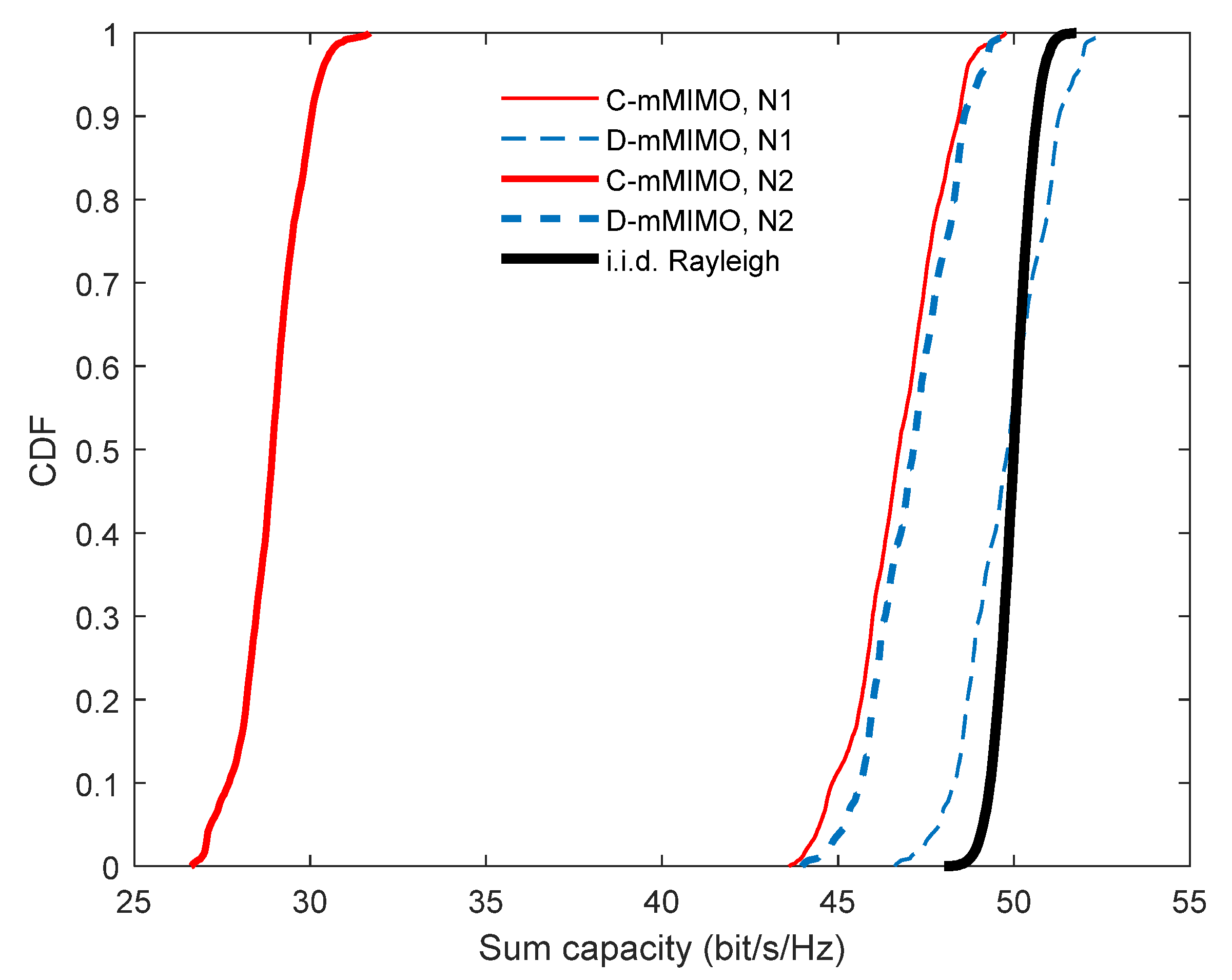
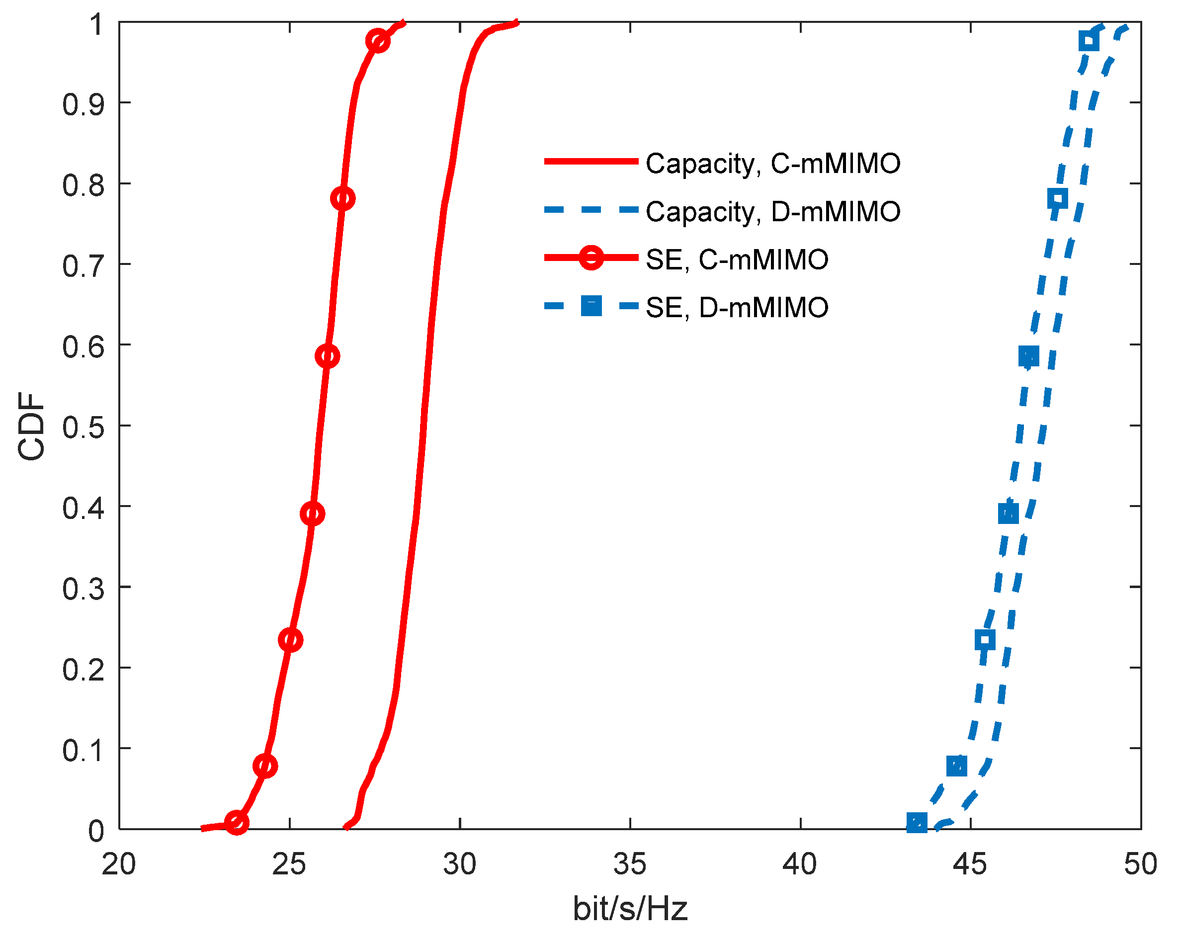
Taking as a reference empirical data obtained from channel measurements carried out in an indoor cell, a comparison between D-mMIMO and C-mMIMO systems as deployment alternatives has been reported and discussed. The channel measurements have been performed in the frequency domain, considering a 400 MHz span centered at 3.5 GHz.

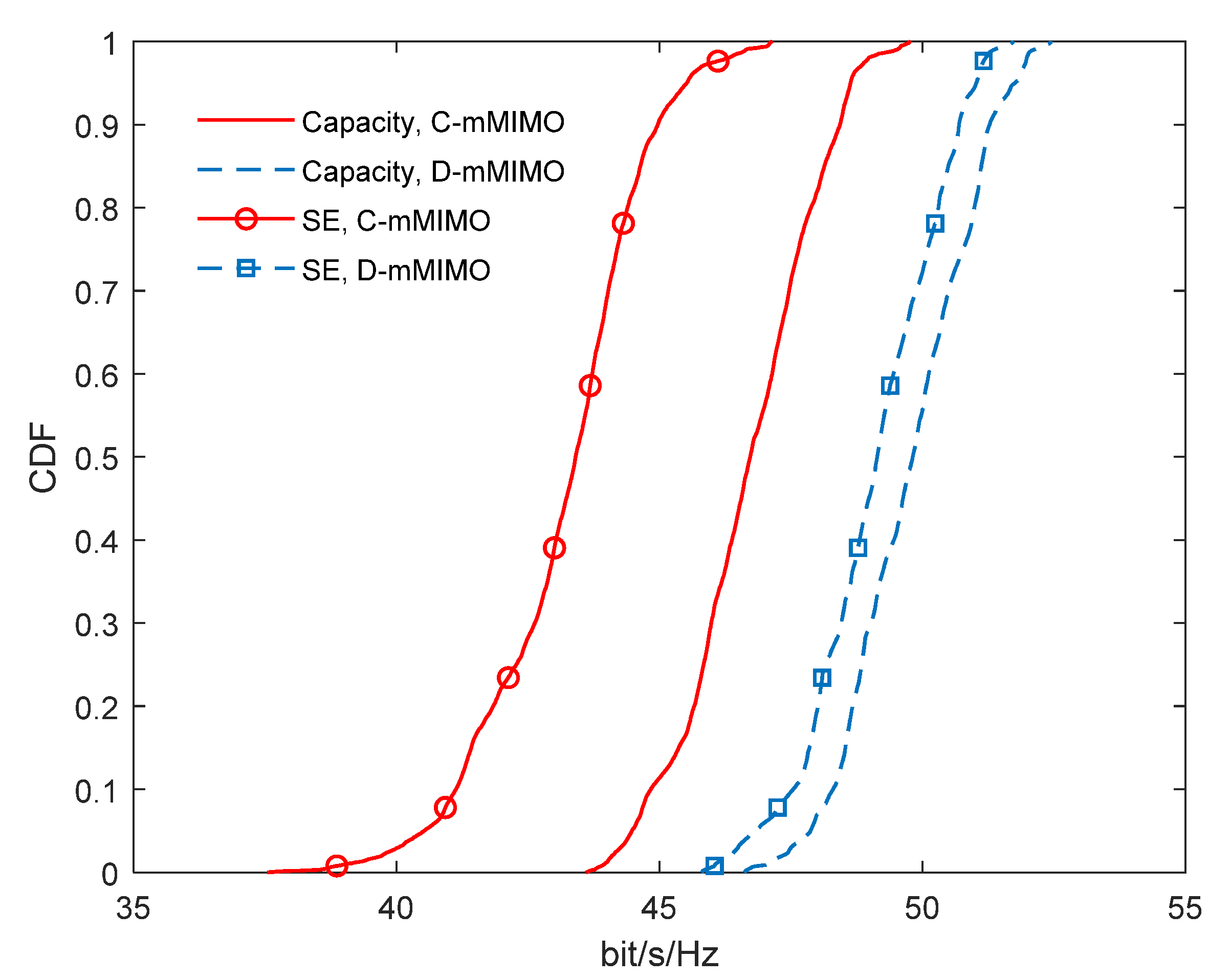
The results show that the sum capacity of the D-mMIMO channel always outperforms that achieved by the C-mMIMO channel. In fact, in the particular case of not performing a power control mechanism, the C-mMIMO sum capacity is much lower than that of the D-mMIMO system. The explanation for such differences is obtained from the analysis of the ICN performance and the power imbalance between the sub-channels for both systems. In the case of the C-mMIMO channel, low ICN values are obtained, even in the case of compensating for the power imbalance between sub-channels. On the contrary, in the case of the D-mMIMO channel, the ICN values are always higher, and in the case of performing an ideal power control, they are close to those of an i.i.d. Rayleigh reference channel. Although the power control applied in this work is ideal, it can be inferred that the C-mMIMO channel will always be more dependent on the realistic power control that could be carried out than the D-mMIMO one.

The sum SE reflects the characteristics of the channel that explain the behavior of the capacity. It is observed that the sum SE is always greater for the D-mMIMO system. It can also be stated that the loss of SE with respect to the obtainable capacity is considerably higher for the C-mMIMO system than for the D-mMIMO one. The difference between the SE and the capacity depends on the performance of the ZF combination method. Although ZF removes the interference generated by other users, the application of this combination method introduces an additional noise enhancement. This problem, which degrades the SE, has a greater impact on channels with ill-conditioned G matrices, as is the case of the concentrated channel versus the distributed one, as confirmed from the observation of the measured ICN performance.

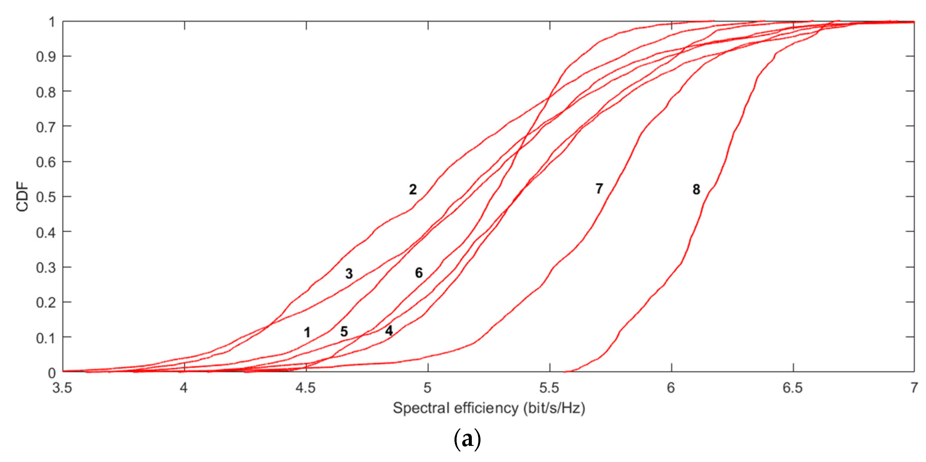
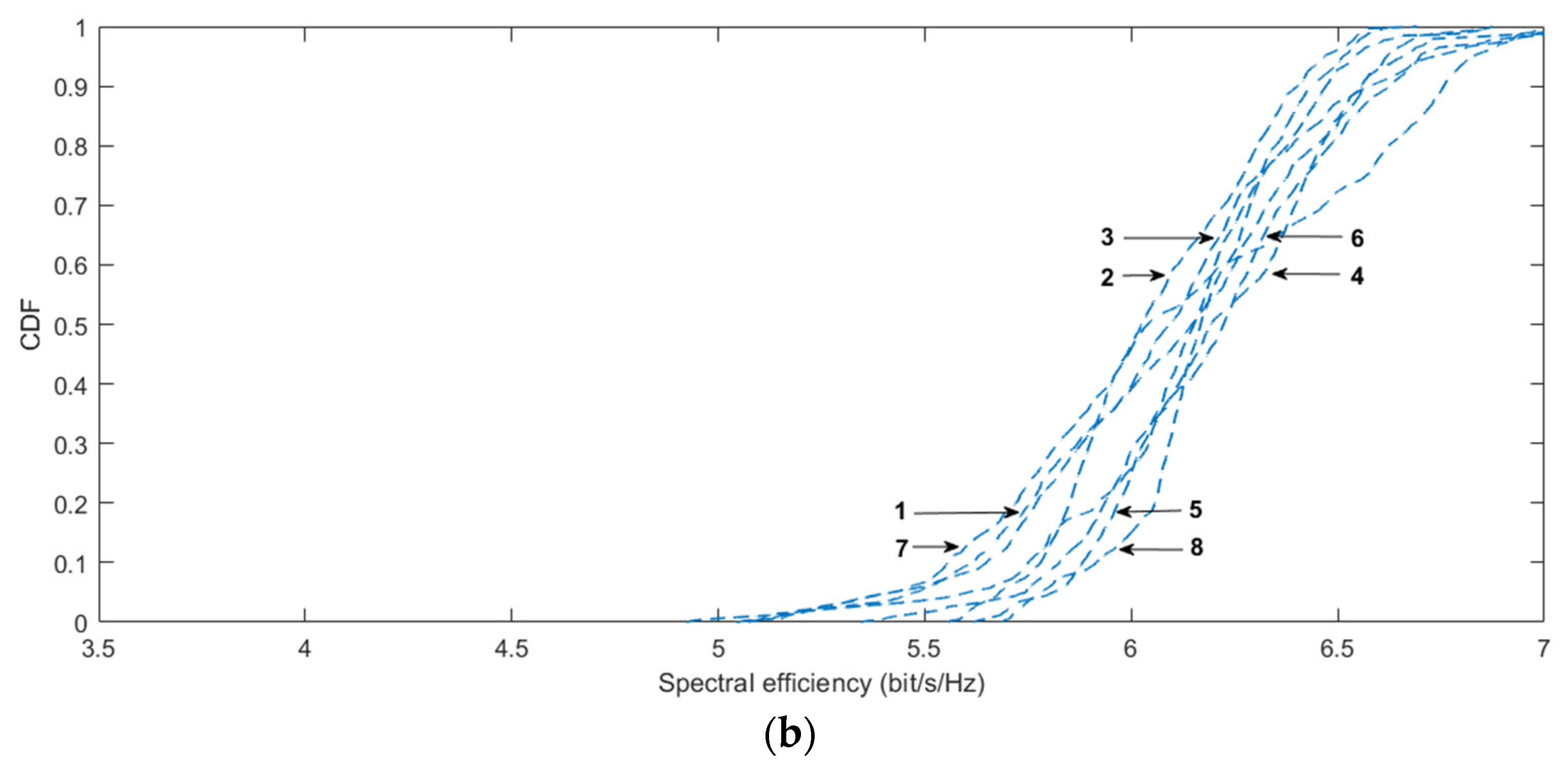
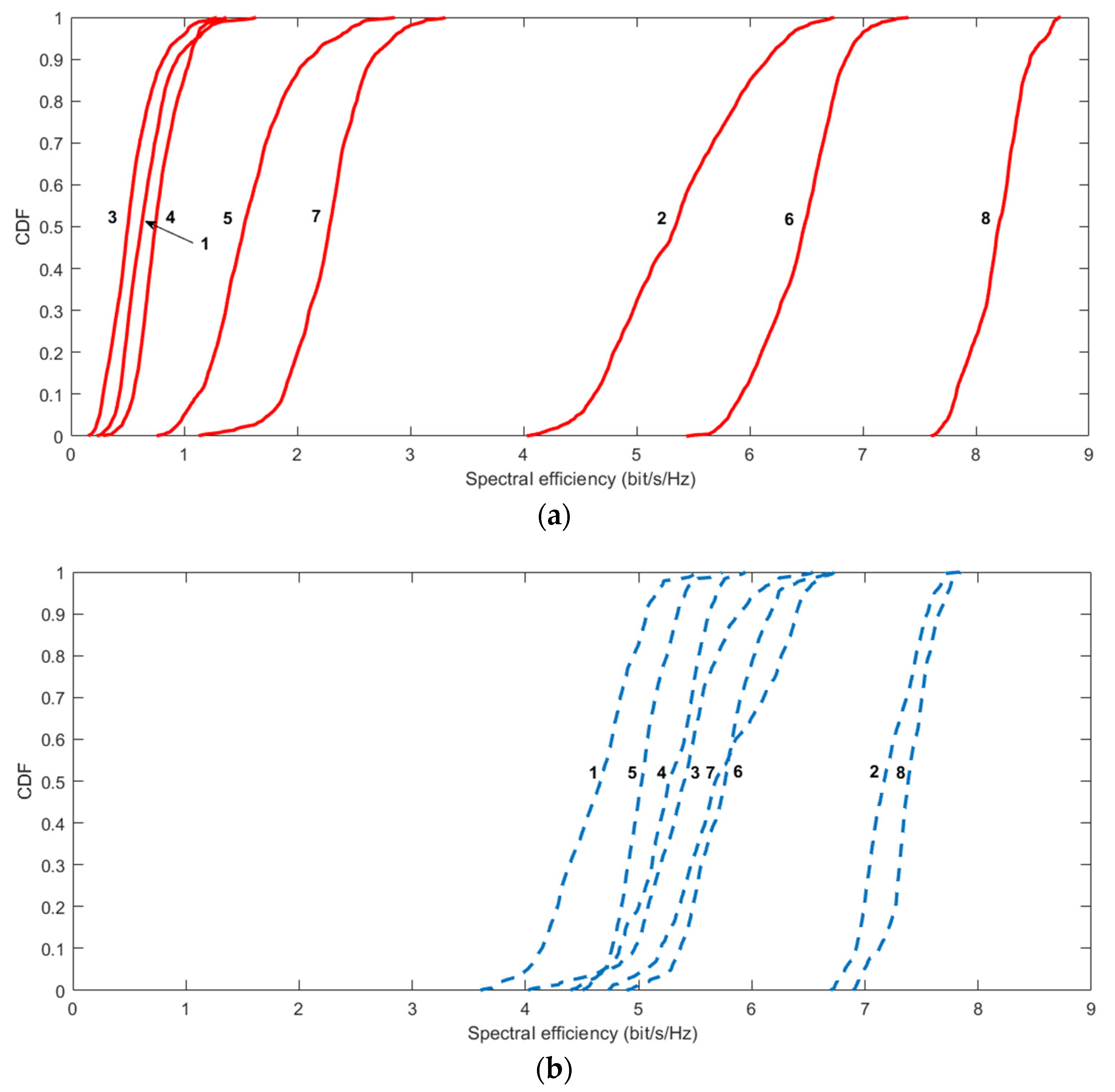
Finally, an important parameter in the comparison between both systems is the user fairness. The paper presents the CDF of the SE of each user, and these are related to the distance and degree of obstruction (LOS or NLOS) of each one. Furthermore, the user fairness is quantified with Jain’s Fairness Index. In conclusion, it can be stated that in the case of not performing a power control, the SE of the users is clearly more homogeneous in the D-mMIMO system than in the C-mMIMO one. When a perfect power control is carried out, the situation is equalized between both systems. Nevertheless, it is important to emphasize again that the behavior of this parameter will be much more dependent on the effective power control that can be implemented in practice in a concentrated system than in a distributed one.

References

1. Björnson, E.; Sanguinetti, L.; Wymeersch, H.; Hoydis, J.; Marzetta, T.L. Massive MIMO is a reality—What is next?: Five promising research directions for antenna arrays. Digit. Signal Process. 2019, 94, 3–20. [Google Scholar] [CrossRef]
2. Clark, M.V.; Willis, T.M.; Greenstein, L.J.; Rustako, A.J.; Erceg, V.; Roman, R.S. Distributed versus centralized antenna arrays in broadband wireless networks. In Proceedings of the IEEE VTS 53rd Vehicular Technology Conference, Rhodes, Greece, 6–9 May 2001; pp. 33–37. [Google Scholar] [CrossRef]
3. Shamai, S.; Zaidel, B.M. Enhancing the cellular downlink capacity via co-processing at the transmitting end. In Proceedings of the IEEE VTS 53rd Vehicular Technology Conference, Rhodes, Greece, 6–9 May 2001; pp. 1745–1749. [Google Scholar] [CrossRef]
4. Zhou, S.; Zhao, M.; Xu, X.; Wang, J.; Yao, Y. Distributed wireless communication system: A new architecture for future public wireless access. IEEE Commun. Mag. 2003, 41–43, 108–113. [Google Scholar] [CrossRef]
5. Dai, L. A Comparative Study on Uplink Sum Capacity with Co-Located and Distributed Antennas. IEEE J. Sel. Areas Commun. 2011, 29, 1200–1213. [Google Scholar] [CrossRef]
6. Zhang, H.; Dai, H. On the Capacity of Distributed MIMO Systems. In Proceedings of the Conference on Information Sciences and Systems, Princeton, NJ, USA, 17–19 March 2004. [Google Scholar]
7. Dai, H. Distributed Versus Co-Located Mimo Systems with Correlated Fading and Shadowing. In Proceedings of the IEEE International Conference on Acoustics Speech and Signal Processing Proceedings, Toulouse, France, 14–19 May 2006; p. IV. [Google Scholar] [CrossRef]
8. Dai, H.; Zhang, H.; Zhou, Q. Some analysis in distributed MIMO systems. J. Commun. 2007, 2. [Google Scholar] [CrossRef]
9. Amiri, A.; Angjelichinoski, M.; de Carvalho, E.; Heath, R.W. Extremely Large Aperture Massive MIMO: Low Complexity Receiver Architectures. In Proceedings of the IEEE Globecom Workshops (GC Wkshps), Abu Dhabi, United Arab Emirates, 9–13 December 2018; pp. 1–6. [Google Scholar] [CrossRef] [Green Version]
10. Almelah, H.B.; Hamdi, K.A. Spectral Efficiency of Distributed Large-Scale MIMO Systems with ZF Receivers. IEEE Trans. Veh. Technol. 2017, 66, 4834–4844. [Google Scholar] [CrossRef]
11. Ngo, H.Q.; Ashikhmin, A.; Yang, H.; Larsson, E.G.; Marzetta, T.L. Cell-Free Massive MIMO versus Small Cells. IEEE Trans. Wirel. Commun. 2017, 16, 1834–1850. [Google Scholar] [CrossRef] [Green Version]
12. Nayebi, E.; Ashikhmin, A.; Marzetta, T.L.; Yang, H.; Rao, B.D. Precoding and Power Optimization in Cell-Free Massive MIMO Systems. IEEE Trans. Wirel. Commun. 2017, 16, 4445–4459. [Google Scholar] [CrossRef]
13. Björnson, E.; Sanguinetti, L. Making Cell-Free Massive MIMO Competitive with MMSE Processing and Centralized Implementation. IEEE Trans. Wirel. Commun. 2020, 19, 77–90. [Google Scholar] [CrossRef] [Green Version]
14. You, X.; Wang, D.; Wang, J. Distributed MIMO and Cell-Free Mobile Communication; Springer: Singapore, 2021. [Google Scholar] [CrossRef]
15. Héliot, F.; Hoshyar, R.; Tafazolli, R. An Accurate Closed-Form Approximation of the Distributed MIMO Outage Probability. IEEE Trans. Wirel. Commun. 2011, 10, 5–11. [Google Scholar] [CrossRef] [Green Version]
16. Lee, S.; Moon, S.; Kim, J.; Lee, I. Capacity Analysis of Distributed Antenna Systems in a Composite Fading Channel. IEEE Trans. Wirel. Commun. 2012, 11, 1076–1086. [Google Scholar] [CrossRef]
17. Wang, D.; Wang, J.; You, X.; Wang, Y.; Chen, M.; Hou, X. Spectral Efficiency of Distributed MIMO Systems. IEEE J. Sel. Areas Commun. 2013, 31, 2112–2127. [Google Scholar] [CrossRef]
18. Li, X.; Li, L.; Su, X.; Wang, Z.; Zhang, P. Approximate capacity analysis for distributed MIMO system over Generalized-K fading channels. In Proceedings of the IEEE Wireless Communications and Networking Conference (WCNC), New Orleans, LA, USA, 9–12 March 2015; pp. 235–240. [Google Scholar] [CrossRef]
19. Chen, C.; Guevara, A.P.; Pollin, S. Scaling up distributed massive MIMO: Why and how. In Proceedings of the 51st Asilomar Conference on Signals, Systems, and Computers, Pacific Grove, CA, USA, 29 October–1 November 2017; pp. 271–276. [Google Scholar] [CrossRef]
20. Chen, C.-M.; Wang, Q.; Gaber, A.; Guevara, A.P.; Pollin, S. User Scheduling and Antenna Topology in Dense Massive MIMO Networks: An Experimental Study. IEEE Trans. Wirel. Commun. 2020, 19, 6210–6223. [Google Scholar] [CrossRef]
21. Okuyama, T.; Suyama, S.; Mashino, J.; Okumura, Y.; Shiizaki, K.; Akiyama, C.; Tsutsui, M.; Seki, H.; Minowa, M. Antenna Deployment of 5G Ultra High-Density Distributed Massive MIMO by Low-SHF-Band Indoor and Outdoor Experiments. In Proceedings of the IEEE 86th Vehicular Technology Conference (VTC-Fall), Toronto, ON, Canada, 24–27 September 2017; pp. 1–5. [Google Scholar] [CrossRef]
22. Kumagai, S.; Kobayashi, T.; Oyama, T.; Akiyama, C.; Tsutsui, M.; Jitsukawa, D.; Seyama, T.; Dateki, T.; Seki, H.; Minowa, M.; et al. Experimental Trials of 5G Ultra High-Density Distributed Antenna Systems. In Proceedings of the IEEE 90th Vehicular Technology Conference (VTC2019-Fall), Honolulu, HI, USA, 22–25 September 2019; pp. 1–5. [Google Scholar] [CrossRef]
23. Gao, X.; Edfors, O.; Rusek, F.; Tufvesson, F. Massive MIMO performance evaluation based on measured propagation data. IEEE Trans. Wirel. Commun. 2015, 14, 3899–3911. [Google Scholar] [CrossRef] [Green Version]
24. Marzetta, T.L. Noncooperative cellular wireless with unlimited numbers of base station antennas. IEEE Trans. Wirel. Commun. 2010, 9, 3590–3600. [Google Scholar] [CrossRef]
25. Björnson, E.; Larsson, E.G.; Marzetta, T.L. Massive MIMO: Ten myths and one critical question. IEEE Commun. Mag. 2016, 54, 114–123. [Google Scholar] [CrossRef] [Green Version]
26. Bogale, T.E.; Le, L.B. Massive MIMO and mmWave for 5G wireless hetnet. IEEE Veh. Technol. Mag. 2016, 11, 64–75. [Google Scholar] [CrossRef]
27. Rusek, F.; Persson, D.; Lau, B.K.; Larsson, E.G.; Marzetta, T.L.; Edfors, O.; Tufvesson, F. Scaling up MIMO: Opportunities and challenges with very large arrays. IEEE Signal Process. Mag. 2013, 30, 40–60. [Google Scholar] [CrossRef] [Green Version]
28. Jain, R.K.; Chiu, D.-M.W.; Hawe, W.R. A Quantitative Measure of Fairness and Discrimination; Eastern Research Laboratory, Digital Equipment Corporation: Hudson, MA, USA, 1984. [Google Scholar]
29. Pérez, J.R.; Torres, R.P.; Domingo, M.; Valle, L.; Basterrechea, J. Analysis of Massive MIMO Performance in an Indoor Picocell with High Number of Users. IEEE Access 2020, 8, 107025–107034. [Google Scholar] [CrossRef]
30. Parsons, J.D. Wideband Channel Characterization. The Mobile Radio Propagation Channel, 2nd ed.; John Wiley & Sons: Hoboken, NJ, USA, 2000; Chapter 6; pp. 164–189. [Google Scholar]
31. Larson, E.G. MIMO detection methods: How they work. IEEE Signal Process. Mag. 2009, 26, 91–95. [Google Scholar] [CrossRef] [Green Version]
Figure 1. Top view of the indoor office environment: (a) General overview of the measurement environment; (b) Zoom of the central part of the floor considered in the experimental analysis, including positions for both UTs and receiver trajectories.
Electronics 10 01646 g001
Figure 2. Schematic of the concentrated massive multiple-input multiple-output (C-mMIMO) channel sounder: (a) Detail of the measurement setup; (b) Block diagram of the channel sounding system.
Electronics 10 01646 g002
Figure 3. Schematic of the distributed massive multiple-input multiple-output (D-mMIMO) channel sounder: (a) Detail of the measurement setup; (b) Block diagram of the channel sounding system.
Electronics 10 01646 g003
Figure 4. CDF of the sum capacity considering concentrated and distributed MIMO systems, along with the normalizations N1 and N2. The i.i.d. Rayleigh channel result is included as a reference.
Electronics 10 01646 g004
Figure 5. CDF of the Inverse Condition Number for C-mMIMO and D-mMIMO channels, along with the two normalizations, N1 and N2. The i.i.d. Rayleigh channel result is included as a reference.
Electronics 10 01646 g005
Figure 6. Expected value, E { g q 2 } , considering concentrated and distributed MIMO systems, along with N1 and N2 normalizations.
Electronics 10 01646 g006
Figure 7. CDF comparing the sum spectral efficiency and sum capacity for both C-mMIMO and D-mMIMO channels when considering the N1 normalization.
Electronics 10 01646 g007
Figure 8. CDF of the spectral efficiency for every UT, comparing both (a) C-mMIMO and (b) D-mMIMO systems, when the N1 normalization is applied.
Electronics 10 01646 g008aElectronics 10 01646 g008b
Figure 9. CDF comparing the sum spectral efficiency and sum capacity for both C-mMIMO and D-mMIMO channels when considering the N2 normalization.
Electronics 10 01646 g009
Figure 10. CDF of the spectral efficiency for every UT, comparing both (a) C-mMIMO and (b) D-mMIMO systems, when the N2 normalization is applied.
Electronics 10 01646 g010