Article

Distance Measurement of Unmanned Aerial Vehicles Using Vision-Based Systems in Unknown Environments

1
Department of Electrical Engineering, National Central University, Zhongli 32001, Taiwan
2
Faculty of Integrated Technologies, Universiti Brunei Darussalam, Jalan Tungku Link, Gadong BE1410, Brunei
3
Department of Automatic Control and Robotics, AGH University of Science and Technology, 30-059 Kraków, Poland
4
Department of Electrical Engineering, Cracow University of Technology, Warszawska 24 Str., 31-155 Cracow, Poland
5
Electrical Engineering Department, College of Engineering, Najran University, Najran 61441, Saudi Arabia
*
Authors to whom correspondence should be addressed.
Electronics 2021, 10(14), 1647; https://doi.org/10.3390/electronics10141647
Submission received: 25 May 2021 / Revised: 4 July 2021 / Accepted: 8 July 2021 / Published: 10 July 2021
(This article belongs to the Section Microwave and Wireless Communications)

Abstract

:
Localization for the indoor aerial robot remains a challenging issue because global positioning system (GPS) signals often cannot reach several buildings. In previous studies, navigation of mobile robots without the GPS required the registration of building maps beforehand. This paper proposes a novel framework for addressing indoor positioning for unmanned aerial vehicles (UAV) in unknown environments using a camera. First, the UAV attitude is estimated to determine whether the robot is moving forward. Then, the camera position is estimated based on optical flow and the Kalman filter. Semantic segmentation using deep learning is carried out to get the position of the wall in front of the robot. The UAV distance is measured using the comparison of the image size ratio based on the corresponding feature points between the current and the reference of the wall images. The UAV is equipped with ultrasonic sensors to measure the distance of the UAV from the surrounded wall. The ground station receives information from the UAV to show the obstacles around the UAV and its current location. The algorithm is verified by capture the images with distance information and compared with the current image and UAV position. The experimental results show that the proposed method achieves an accuracy of 91.7% and a computation time of 8 frames per second (fps).

1. Introduction

Nowadays, there has been an increase in unmanned aerial vehicles (UAV) to be used in various fields for different applications of indoor [1] and outdoor [2,3] surveillance investigation. Aerial surveillance [4] has the advantages of avoiding some obstacles and uneven surfaces on the land, where the positioning of the UAV mostly relies on the global positioning system (GPS) [2]. However, GPS signals can be easily disturbed and cannot reach some places, such as urban areas, mountains, forests, and buildings [5]. This situation makes localization of UAVs without the GPS remain a challenging task.
In simultaneous localization and mapping (SLAM) [6], the mapping system is a crucial component for UAV localization and navigation, such as point cloud maps [7] and occupancy maps [8]. Point cloud maps can be obtained by combining point measurements. However, this type of map is only suitable for high-precision sensors in static environments, because in the new environment, object mapping cannot be accessed and modified. The main limitation of occupancy maps is the fixed-size voxel grid that requires a map size that is known in advance and cannot be changed dynamically. Thus, these mapping methods cannot be used in a new and unknown environment. So, one of the more precise ways to find out the current position of the robot in a building is to calculate its current distance from the entrance.
Several methods have been proposed to determine the location of mobile robots by measuring distances using radio frequency (RF) and sensors. Ni et al. [9] and Guerrieri et al. [10] presented an indoor localization system using radio frequency identification (RFID). RFID-based localization uses RF tags placed on buildings as navigation waypoints and tracking tags that are attached to moving objects, so readers can track the objects in different locations. However, these methods require many expensive RFID readers, and the detection capability of each tag only works for about 6 m. A localization method based on the laser finder was proposed by Subramanian et al. [11] and Barawid et al. [12], mounted on a vehicle as a navigation sensor. The laser finder was used to obtain distance information to explore the surrounding environment and avoid obstacles. However, these methods have high hardware costs and a heavy load that is not suitable for UAVs. A Zigbee-based system for obtaining the location of the user and tracking them inside a building was introduced by Lin et al. [13]. Zigbee devices are set up beforehand in the building, and the target movement is assumed to be constant. Cheok et al. [14] developed a method for indoor positioning and navigation using light sensors. Still, this method requires installing fluorescent lamps in buildings and hardware for use by users or moving objects. Nakahira et al. [15] proposed the concept of distance measurement using the ultrasonic system to determine the position and orientation of mobile robots in a room. This method measures distance by processing the signal from the returning echoes of the acoustic pulse emitted into space. It is not suitable for long-distance measurement and is only used to avoid obstacles near the robots.
Previous studies on indoor positioning used a vision-based system to solve the localization problem of mobile robots. By using visual sensors, environmental information in the form of color, texture, and other visual information can be obtained more easily and accurately compared to the GPS, laser flashes, ultrasonic sensors, and other traditional sensors. In addition, visual sensors are also cheaper and easier to use, so vision-based navigation is one of the techniques that has continued to be developed recently. Kim et al. [16] used an augmented reality technology to provide location information in indoor environments. However, this method only recognizes a particular location by a marker that has a characteristic pattern. Li et al. [17] presented a localization method by distance measurement using a webcam placed inside a building. Due to the low-quality lens and brightness changes in the structure, the images taken had low quality. So, the camera needed calibration to avoid image distortion problems [18]. In [17], a mobile robot was first detected to determine its coordinates on the image. Then, the location of the robot was estimated based on the distance between the camera and the position of the wall near the robot. Shim et al.’s [19] approach used coordinate mapping to recognize robots in a building using multiple cameras at the same time. Lan et al. [20] conducted research on vision-based navigation schemes for UAVs based on mapped landmarks, where absolute positions of the landmark points are known.
The main purpose of this paper is to create a new framework to determine the location of a UAV based on distance measurements using a single camera. In this study, the camera mounted on the UAV transmits the image wirelessly to the ground station. This method is proposed as a solution for positioning and navigation of UAVs in indoor environments where the location map is not registered and without devices installed beforehand. The distance is measured by a size comparison between reference and current images. Then, the UAV movement is mapped in the user interface.
The remainder of this paper is organized as follows. Section 2 provides an explanation of the proposed material and the main algorithms. Section 3 provides performance results using videos captured from the UAV, supplemented by a discussion. Next, Section 4 summarizes the conclusions.

2. Materials and Methods
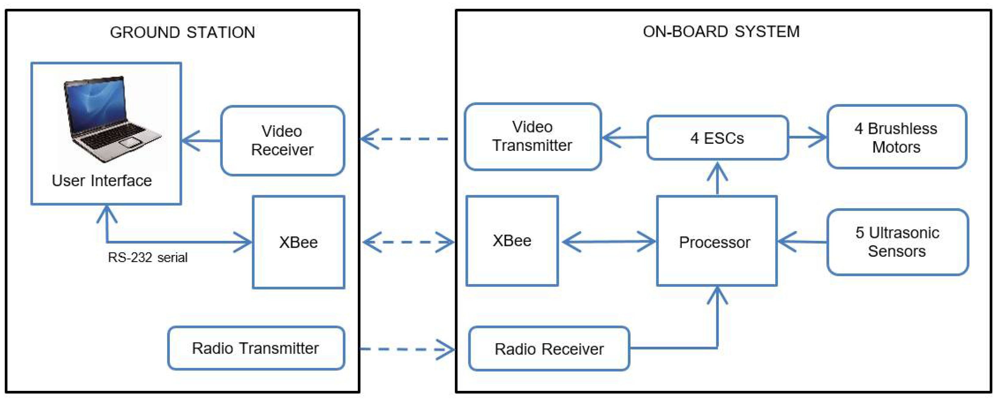
2.1. Materials

The experiments were carried out using Visual Studio as the software program in a 3.40 GHz CPU with 8 GB RAM. Aerial image sequences with a resolution of 720 × 480 were taken to implement the proposed method. Figure 1 shows an overview system of the UAV and the ground station. The type of UAV used in this system is a quadrotor consisting of four rotors where the radio receiver receives flight commands. Each rotor speed is controlled via an electronic speed controller (ESC) that receives a signal from the processor. The XBee module on the onboard system has the function to send UAV flight data to the ground station. An ultrasonic sensor is installed on each side of the quadrotor frame to detect obstacles when the quadrotor flies, and one sensor is mounted with the camera.

2.2. The Proposed Methods

The algorithm consists of several steps: UAV attitude estimation, camera position correction, semantic segmentation, and distance measurement. First, when the UAV moves around 3 m from the starting point, the reference image I is captured. The distance of the UAV from the starting point is measured using ultrasonic sensors mounted with the camera. The UAV attitude is estimated to determine the current pitch angle of the UAV. If the pitch angle is positive, it means that the UAV is moving forward. Figure 2 shows an overview of the system proposed in this paper.
Then, for every 100 ms, the current image is captured and aligned based on the camera position estimation. The semantic segmentation is performed to determine the location of the wall in front of the UAV as a current image. The first wall frame is saved as a reference frame. Then, the feature points in the reference and current images are found to obtain an affine transformation of the current image. So, a size comparison between the reference and current images can be obtained. If the reference image size is less than 55% of the current image, then it is assumed that the UAV has moved 1 m forward. Then, the reference image is updated every 1 m. In this work, the UAV moves with a speed of around 1–1.5 m/s, and we assume that the UAV moves at a constant altitude and speed.

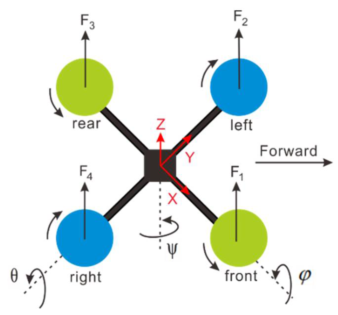
2.3. UAV Attitude Estimation

Figure 3 shows that the front and rear rotors rotate clockwise, and the others rotate counter-clockwise. A force Fi is generated by each rotor i and is used to calculate the Euler angles: roll ϕ , pitch θ , and yaw ψ . The main thrust FN and control input, which depends on the rotor profile, can be calculated as follows [21]:
F N = i = 1 4 | F i | = C t h ( i = 1 4 ω i 2 )
{ U 1 = F 1 + F 3 + F 2 + F 4 U 2 = F 4 F 2 U 3 = F 3 F 1 U 4 = C d ( F 1 + F 3 F 2 F 4 )
FN is applied to the airframe, where C t h is the thrust coefficient of each rotor, ω i is the angular velocity of rotor I, and C d is the drag coefficient.
The gyroscope and accelerometer measure three angular rates and two angular positions ( ϕ and θ ) where the magnetometer measures ψ . A nonlinear complementary filter on the SO(3) [22] is used on each axis of the accelerometer and gyroscope to estimate the UAV attitude. Figure 4 shows the position and orientation of the UAV, where {E} is an arbitrary point of the space with a fixed inertial frame x, y, and z axes; l is the arm length of the UAV; m is mass; and g is the gravitational acceleration. Then, the dynamic model of the UAV is computed as follows [23,24]:
{ ϕ ¨ = ( J y J z J x ) θ ˙ ψ ˙ + l J x U 2 θ ¨ = ( J z J x J y ) ϕ ˙ θ ˙ + l J y U 3 ψ ¨ = ( J x J y J z ) ϕ ˙ θ ˙ + 1 J z U 4 x ¨ = 1 m ( cos ϕ sin θ cos ψ + sin ϕ sin ψ ) U 1 y ¨ = 1 m ( cos ϕ sin θ sin ψ sin ϕ cos ψ ) U 1 z ¨ = g 1 m ( cos ϕ cos θ ) U 1
where J x ,   J y ,   and   J z indicate the moments of inertia on the x, y, and z axes, respectively.

2.4. Camera Position Correction

This step estimates the camera position to align the current image. Figure 5 shows an illustration of UAV movement that affects the camera motion. The image motion corresponds to camera motion on the yaw, pitch, and roll axes of the UAV movement. The affine transformation is used to handle the rotation and translation of the images.
The optical flow method in [26] is used in this step to calculate the motion vectors of two consecutive frames. For each 10 × 10 sub-window, the flow of each pixel in the window is estimated by a polynomial in the local coordinate system (LCS) at I as follows:
I L C S p = p T A p + b T p + c
where p is a vector, A is a symmetric matrix, b is a vector, and c is a scalar. The LCS at I ( t ) can be defined by
I L C S p ( t ) = p T A ( t ) p + b T ( t ) p + c ( t )
Based on Equations (4) and (5), a new signal can be built at I ( t ) by a global displacement Δ ( t ) as I L C S p ( t ) = I L C S p Δ ( t ) , so the relation between the LCS of two input images can be calculated by
I L C S p ( t ) = ( p Δ ( t ) ) T A ( p Δ ( t ) ) + b T ( p Δ ( t ) ) + c
The coefficients of b in Equations (5) and (6) can be equated by
b ( t ) = b 2 A Δ ( t )
So, the total displacement of the motion vectors in I ( t ) is computed as follows:
Δ ( t ) = 1 2 A 1 ( b ( t ) b )
The displacement value in Equation (8) is the translation of the motion vectors containing of the x axis ( Δ x ( t ) ) and y axis ( Δ y ( t ) ) , so its angular value can be calculated by
Δ θ ( t ) = tan 1 ( Δ ( y ) ( t ) Δ ( x ) ( t ) ) × 180 π
Then, the translation T x , y ( t ) and rotation θ ( t ) of I ( t ) are obtained as the most frequent value of the motion vectors as follows:
T x , y ( t ) = l Δ ( t ) + ( f 1 Δ ( t ) f 2 Δ ( t ) 2 f 1 Δ ( t ) f 0 Δ ( t ) f 2 Δ ( t ) ) × τ
and
θ ( t ) = l Δ θ ( t ) + ( f 1 Δ θ ( t ) f 2 Δ θ ( t ) 2 f 1 Δ θ ( t ) f 0 Δ θ ( t ) f 2 Δ θ ( t ) ) × τ
where l is the lower motion vector value, τ is the size of the motion vector class interval, f 1 is the frequency of the modal class, f 0 is the frequency of the class preceding the modal class, and f 2 is the frequency of the class succeeding the modal class.
In the next step, the translation and rotation obtained are compensated using the Kalman filter consisting of prediction and measurement parts. The initial state in the prediction step is defined by s ( 0 ) = [ 0 , 0 , 0 ] , and then the state of the trajectory s ^ ( t ) = [ T ^ x ( t ) , T ^ y ( t ) , θ ^ ( t ) ] at I ( t ) can be estimated by
s ^ ( t ) = s ( t 1 )
The initial error covariance in the prediction step is defined by e ( 0 ) = [ 1 , 1 , 1 ] , where the error covariance computed by
e ^ ( t ) = e ( t 1 ) + Q p
where Q p is the process’s noise covariance set to 0.004. A Kalman gain can be calculated by
K ( t ) = e ^ ( t ) e ^ ( t ) + Q m ,
where Q m is the measurement’s noise covariance set to 0.25. The error covariance compensation is calculated as follows:
e ( t ) = ( 1 K ( t ) ) e ^ ( t )
Then, the trajectory is compensated in the new state by s ( t ) = [ T x ( t ) , T y ( t ) , θ ( t ) ] , where the trajectory state at I ( t ) is calculated as follows:
s ( t ) = s ^ ( t ) + K ( t ) ( R ( t ) s ^ ( t ) )
The accumulation of the trajectory from each frame can be measured by
R ( t ) = r = 1 t 1 [ ( T ¯ x ( r ) + T x ( t ) ) , ( T ¯ x ( r ) + T x ( t ) ) , ( θ ¯ ( r ) + θ ( t ) ) ] = [ R x ( t ) , R y ( t ) , R θ ( t ) ]
So, a new trajectory can be obtained as follows:
[ T ¯ x ( t ) , T ¯ y ( t ) , θ ¯ ( t ) ] = [ T x ( t ) , T y ( t ) , θ ( t ) ] + [ d x ( t ) , d y ( t ) , d θ ( t ) ]
where the difference between x, y, and θ can be obtained as d x ( t ) = T x ( t ) R x ( t ) , d y ( t ) = T y ( t ) R ( t ) , and d θ ( t ) = θ ( t ) R θ ( t ) , respectively.
Finally, a new image plane is produced to apply the new trajectory in Equation (18) to align I ( t ) with the transformation as follows:
I ¯ ( t ) = I ( t ) × [ cos θ ¯ ( t ) sin θ ¯ ( t ) sin θ ¯ ( t ) cos θ ¯ ( t ) ] + [ T ¯ x ( t ) T ¯ y ( t ) ]

2.5. Semantic Segmentation

We implemented a deep convolutional neural network (DCNN) [27] with ResNet-101 [28] for segmenting indoor scenes on ade20 k datasets. The model used is shown in Figure 6. To double the spatial density, feature responses are computed in the ResNet-101 network, then the last pooling or convolution layer is found to lower resolution. To determine the area of floors, walls, roofs, and other furniture in the room, we created labels for 27 classes in order to easily classify obstacles and roads in front of the robot. Fully connected layers are transformed into convolutional layers with increased feature resolution so that the feature response can be computed for every 8 pixels. Bi-linear interpolation is performed to resize the score map to the original image resolution. Then, the input image is forwarded to a fully connected CRF [29] to fine-tune the segmentation results.

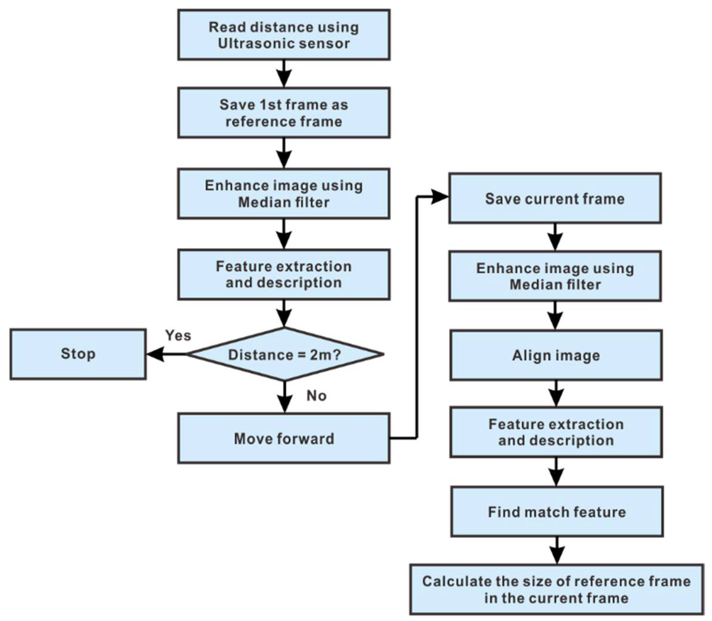
2.6. Distance Measurement

This step estimates the position and size comparison of I at I(t) based on affine transformation [25,30]. The position of features that have similarities between I and I(t) is found using scale-invariant features transform (SIFT) [31]. SIFT is used as the feature extractor and descriptor in this method because it provides more invariance in the illumination changes compared with SURF [32,33].
First, the image color is changed into a gray-scale, and a median filter [34] is applied. Then, interesting points are approximated using Laplacian of Gaussian (LoG) in the scale space images. The difference between two consecutive scales is calculated as the convolution of the scale space with the Gaussian function as follows:
L ( x , y , σ ) = G ( x , y , σ ) I ( x , y )
where G ( x , y , σ ) is a scale-variable Gaussian defined as
G ( x , y , σ ) = 1 2 π σ 2 e ( x 2 + y 2 ) / 2 σ 2
where ( x , y ) are the spatial coordinates and σ is the scale space factor.
The key points are found as the maxima and minima in the difference of Gaussian (DoG) between two images to make it a scale-invariant. This is done by comparing eight neighbor pixels in the current scale and nine corresponding neighbors at neighboring scales. Two such extrema images are generated, which need 4 DoG images with 5 Gaussian blurred images, hence the five levels of blurs in each octave. The DoG function with adjacent scales k can be computed by
D ( x , y , σ ) = ( G ( x , y , k σ ) G ( x , y , σ ) ) I ( x , y ) = L ( x , y , k σ ) L ( x , y , σ )
The bad key points on the edges and low-contrast regions are rejects using second-order Taylor expansion of the D ( x , y , σ ) at sample point X by
D ( X ) = D + D T X X + 1 2 X T 2 D X 2 X
The location of the extreme point can be calculated by taking the derivative of Equation (23) with respect to X as follows:
X = ( 2 D 1 X 2 ) D X
Then, the low-contrast key points can be obtained by
D ( X ) = D + 1 2 D T X X
The key points are eliminated when | D ( X ) | < D 0 makes the algorithm efficient and robust. Then, the key points along with the edge are filtered out by the Hessian matrix as follows:
H m = [ D x x D x y D x y D y y ]
The magnitude and orientation of each key point are calculated to cancel out the effect of orientation to make it rotation-invariant by
M D ( x , y ) = ( L ( x + 1 , y ) L ( x 1 , y ) ) 2 + ( L ( x , y + 1 ) L ( x , y 1 ) ) 2
and
θ D ( x , y ) = tan 1 ( ( L ( x + 1 , y ) L ( x 1 , y ) ) 2 + ( L ( x , y + 1 ) L ( x , y 1 ) ) 2 )
SIFT features are generated with scale and rotation invariance in place. A SIFT descriptor is a characterization of a key point in the spatial histogram of the image gradients. The gradient at each pixel consists of the location of the pixel and the orientation of the gradient. The orientation is quantized into eight spatial coordinates for each cell in a 16 × 16 window. Then, a histogram consisting of 128 bins (16 cells × 8 orientations) is stacked as a single 128-dimensional vector.
The feature point pairs between I and I(t) are selected using the Fast Library for Approximate Nearest Neighbor (FLANN) [35]. Each distance of the pair is calculated using the Euclidean distance. The feature point is classified as a match if the distance is less than 0.6. Four feature points near the boundary in I(t) that are similar to the feature point in I are selected. These feature points are used to estimate the image size comparison. If the matching feature points are less than four, the feature points of the previous I(t) are used.
In the homogenous coordinates, the relationship between four matching feature points between I and I(t) can be estimated by
[ I ( t ) x I ( t ) y ] = H [ I x I y 1 ]
where H is the homogeneous affine matrix that can be defined by
H = [ 1 + a 11 a 12 T h x a 21 1 + a 22 T h y ]
where aij is the parameter of the rotation angular θh, and Thx and Thy are the translation on the x and y axis on the image plane, respectively. Then, the least-squares problem is used to solve the affine matrix. In addition, the Random Sample Consensus (RANSAC) algorithm [36] is used to filter the outliers to find the correct affine transformation.
As a result of the affine matrix, we can obtain the comparison of I in I(t) with the scale factor Ω ( t ) as follows:
Ω ( t ) = cos θ h ( t ) cos ( tan 1 ( sin θ h ( t ) cos θ h ( t ) ) ) ( t )

2.7. Sensor Specifications

An ultrasonic sensor is used to provide information about the distance of nearby objects. The ultrasonic sensor used is HC-SR04 [37], as shown in Figure 7a, which includes a transmitter, a receiver, and control circuits (Vcc, trigger, echo, and GND). HC-SR04 uses an I/O trigger for 10 µs high-level signals by a pulse input from the processor and then sends eight 40 kHz cycle signals and detects returning pulse signals. If the signal returns through a high level, then the distance (in cm) is calculated as
distance = 2 × ( high   level   time 340   m / s )
There are five ultrasonic sensors used in this system connected to a pin connector on an additional board. The trigger and echo pins are connected to analog pins on the processor, switched alternately using ULN 2803A [38].
The XBee pro s2b module [39], as shown in Figure 7b, provides a UART interface to transmit (TX) and receive (RX) data that are connected to the UART pins on the mainboard. The XBee module operates using the Zigbee protocol with a low-power wireless sensor network that requires minimal power and provides reliable data transmission between remote devices.
The video transmitter, as shown in Figure 7c, used is a 2.4 GHz color CMOS camera to sends aerial images to the radio receiver at the ground station. The power supply for the camera requires 9–12 V DC obtained directly from the battery. Table 1 summarizes the component specifications that are used to support the surveillance system.

3. Results

3.1. The User Interface

Visual Basic Net 2017 is used for user interface (UI) software programming, as shown in Figure 8. The proposed user interface is used to save and display aerial images, estimate the attitude of the UAV, receive obstacle information, and map the UAV’s estimated distance. Arduino is used for mainboard software programming.
First, the COM port and baud rate used to access serial communication are selected. The UI displays the attitude data of the UAV, i.e., yaw, pitch, and roll, and simulates the current position of the UAV. The UAV is equipped with a small motor to move the camera forward and down. In the UI, there are settings for turning the camera on or off, as well as moving the camera up or down. The UI also displays a simulation of the current travel path of the UAV and the number of obstacles around the UAV detected by the ultrasonic sensors.

3.2. Frame Size Comparison

We collected images for around 2 m from the starting point in several locations where the first frame was a reference frame, and for every 50 ms, the reference frame’s size was compared with the current frame’s size. Figure 9 shows the steps for pre-processing images to obtain the average size of a reference in the current frame. The current frame is enhanced using a median filter and aligns based on the correction of the camera position, as described in Section 2.4. The features in the reference and current frames are extracted and described to find the match features, as explained in Section 2.6.
Figure 10 shows the results of the frame size comparison of around 2 m. Based on our experiments, the average size of the reference frame in the current frame for a 1 m distance is about 55%. The best distance measurement using the estimated frame size ratio is for every 1 m going forward. In Figure 10, we can see that after the 25th frame, in which the distance is more than 1 m, the frame size ratio does not significantly differ. The influence of our image quality can cause this result.

3.3. Segmentation

Figure 11 shows the semantic segmentation results for the indoor environment. The walls, floors, roofs, and furniture or other objects in the room are displayed in peach, green, gray, and blue colors, respectively. The wall area is chosen as an area other than the floor or in green. Selecting only the wall area improves accuracy in feature detection and recognition at the next step. Because the floor area is too plain for feature detection, it can cause feature recognition errors and increase computation time.

3.4. Distance Measurement

Figure 12 shows the UAV used in this experiment that is equipped with a camera and ultrasonic sensors. The resulting distance measured using the proposed algorithm is compared with the actual distance, as shown in Figure 13. The results of the distance measurement indicate that the proposed algorithm achieves an accuracy rate of 91.7%. Because the current frame is saved for every 100 ms, the computation time is around 8 fps. Although we have low image quality, the proposed algorithm results are good enough to measure the UAV distance from the starting point. So, we can estimate the UAV’s current location in the building.
The proposed algorithm has the best result for distances less than 12 m. After 12 m, because the starting point is too far away, the result of the frame size ratio is less accurate. Maybe this situation occurs due to the low quality of our images. We believe that the proposed algorithm can be used for longer distances using a high-quality camera.

4. Conclusions

A new method for UAV distance measurement using a vision-based system in an unknown environment is presented in this work. The proposed method has a major contribution in measuring the current UAV distance from the starting point to estimate its location in an indoor environment where the GPS cannot be used. The UAV is equipped with several ultrasonic sensors to avoid obstacles. Unwanted motion in aerial images is handled using the image stabilization method. Semantic segmentation based on deep learning is used to obtain the wall position in front of the UAV. The first wall frame is saved as a reference frame to compare its size ratio in the current frame to determine the current distance of the UAV. The reference frame is updated if the distance is detected as 1 m forward. Comparing the results with actual distances, the proposed method can be used to determine the location of mobile robots, especially UAVs, based on distance measurements in buildings or places that cannot use the GPS without prior place registration. The proposed method provides more than 90% accurate results for short UAV mileage measurements in the building. The addition of physical sensors and more accurate feature detection can be done so that better detection can be carried out for longer distances of the UAV.

Author Contributions

Conceptualization, writing—original draft, data curation, methodology, and software, W.R.; formal analysis, writing—review and editing, and project administration, W.-J.W.; formal analysis, writing—review and editing, and funding acquisition, W.C. and A.G.; writing—review and editing, K.O., M.S., and M.I. Page: 14. All authors have read and agreed to the published version of the manuscript.

Funding

This research was funded by the AGH University of Science and Technology (grant no. 16.16.120.773).

Acknowledgments

The authors would like to thank Satoko Abiko at the Shibaura Institute of Technology, Japan, for her suggestions to make this research better and all lab colleagues at the Abiko Laboratory for their assistance in Japan.

Conflicts of Interest

The authors declare no conflict of interest.

References

  1. Cai, S.; Huang, Y.; Ye, B.; Xu, C. Dynamic illumination optical flow computing for sensing multiple mobile robots from a drone. IEEE Trans. Syst. Man Cybern. Syst. 2017, 48, 1370–1382. [Google Scholar] [CrossRef]
  2. Minaeian, S.; Liu, J.; Son, Y.J. Vision-based target detection and localization via a team of cooperative UAV and UGVs. IEEE Trans. Syst. Man Cybern. Syst. 2016, 46, 1005–1016. [Google Scholar] [CrossRef]
  3. Wang, L.; Zhang, Z. Automatic detection of wind turbine blade surface cracks based on UAV-taken images. IEEE Trans. Ind. Electron. 2017, 64, 7293–7309. [Google Scholar] [CrossRef]
  4. Rahmaniar, W.; Rakhmania, A.E. Online digital image stabilization for an unmanned aerial vehicle (UA ). J. Robot. Control 2021, 2, 234–239. [Google Scholar] [CrossRef]
  5. Mebarki, R.; Lippiello, V.; Siciliano, B. Nonlinear visual control of unmanned aerial vehicles in GPS-denied environments. IEEE Trans. Robot. 2015, 31, 1004–1017. [Google Scholar] [CrossRef]
  6. Chen, S.; Chen, H.; Zhou, W.; Wen, C.-Y.; Li, B. End-to-end UAV simulation for visual SLAM and navigation. arXiv 2020, arXiv:2012.00298. [Google Scholar]
  7. Gao, F.; Wu, W.; Gao, W.; Shen, S. Flying on point clouds: Online trajectory generation and autonomous navigation for quadrotors in cluttered environments. J. Field Robot. 2019, 36, 710–733. [Google Scholar] [CrossRef]
  8. Hornung, A.; Wurm, K.M.; Bennewitz, M.; Stachniss, C.; Burgard, W. OctoMap: An efficient probabilistic 3D mapping framework based on octrees. Auton. Robots 2013, 34, 189–206. [Google Scholar] [CrossRef] [Green Version]
  9. Ni, L.M.; Liu, Y.; Lau, Y.C.; Patil, A.P. LANDMARC: Indoor location sensing using active RFID. In Proceedings of the Pervasive Computing and Communications, Fort Worth, TX, USA, 26–26 March 2003; pp. 407–415. [Google Scholar]
  10. Guerrieri, J.R.; Francis, M.H.; Wilson, P.F.; Kos, T.; Miller, L.E.; Bryner, N.P.; Stroup, D.W.; Klein-Berndt, L. RFID-assisted indoor localization and communication for first responders. In Proceedings of the European Conference on Antennas and Propagation, Nice, France, 6–10 November 2006; pp. 1–6. [Google Scholar]
  11. Subramanian, V.; Burks, T.F.; Arroyo, A.A. Development of machine vision and laser radar based autonomous vehicle guidance systems for citrus grove navigation. Comput. Electron. Agric. 2006, 53, 130–143. [Google Scholar] [CrossRef]
  12. Barawid, O.C.; Mizushima, A.; Ishii, K.; Noguchi, N. Development of an autonomous navigation system using a two-dimensional laser scanner in an orchard application. Biosyst. Eng. 2007, 96, 139–149. [Google Scholar] [CrossRef]
  13. Lin, T.H.; Huang, P.; Chu, H.H.; You, C.W. Energy-efficient boundary detection for RF-based localization systems. IEEE Trans. Mob. Comput. 2009, 8, 29–40. [Google Scholar] [CrossRef] [Green Version]
  14. Cheok, A.D.; Yue, L. A novel light-sensor-based information transmission system for indoor positioning and navigation. IEEE Trans. Instrum. Meas. 2011, 60, 290–299. [Google Scholar] [CrossRef]
  15. Nakahira, K.; Kodama, T.; Morita, S.; Okuma, S. Distance measurement by an ultrasonic system based on a digital polarity correlator. IEEE Trans. Instrum. Meas. 2001, 50, 1748–1752. [Google Scholar] [CrossRef]
  16. Kim, J.; Jun, H. Vision-based location positioning using augmented reality for indoor navigation. IEEE Trans. Consum. Electron. 2008, 54, 954–962. [Google Scholar] [CrossRef]
  17. Li, I.H.; Chen, M.C.; Wang, W.Y.; Su, S.F.; Lai, T.W. Mobile robot self-localization system using single webcam distance measurement technology in indoor environments. Sensors 2014, 14, 2089–2109. [Google Scholar] [CrossRef] [Green Version]
  18. Chen, H.; Matsumoto, K.; Ota, J.; Arai, T. Self-calibration of environmental camera for mobile robot navigation. Rob. Auton. Syst. 2007, 55, 177–190. [Google Scholar] [CrossRef]
  19. Shim, J.H.; Cho, Y.I. A mobile robot localization via indoor fixed remote surveillance cameras. Sensors 2016, 16, 195. [Google Scholar] [CrossRef] [Green Version]
  20. Huang, L.; Song, J. Research of autonomous vision-based absolute navigation for unmanned aerial vehicle. In Proceedings of the Control, Automation, Robotics and Vision (ICARCV), Phuket, Thailand, 13–15 November 2016; pp. 13–15. [Google Scholar]
  21. Mahony, R.; Kumar, V.; Corke, P. Multirotor aerial vehicles: Modeling, estimation, and control of quadrotor. IEEE Robot. Autom. Mag. 2012, 19, 20–32. [Google Scholar] [CrossRef]
  22. Mahony, R.; Hamel, T.; Pflimlin, J.-M. Nonlinear complementary filters on the special orthogonal group. IEEE Trans. Autom. Control 2008, 53, 1203–1218. [Google Scholar] [CrossRef] [Green Version]
  23. Wang, H.; Ye, X.; Tian, Y.; Zheng, G.; Christov, N. Model-free-based terminal SMC of quadrotor attitude and position. IEEE Trans. Aerosp. Electron. Syst. 2016, 52, 2519–2528. [Google Scholar] [CrossRef]
  24. Xuan-Mung, N.; Hong, S.K. Improved altitude control algorithm for quadcopter unmanned aerial vehicles. Appl. Sci. 2019, 9, 2122. [Google Scholar] [CrossRef] [Green Version]
  25. Rahmaniar, W.; Wang, W.; Chen, H. Real-time detection and recognition of multiple moving objects for aerial surveillance. Electronics 2019, 8, 1373. [Google Scholar] [CrossRef] [Green Version]
  26. Farneback, G. Two-frame motion estimation based on polynomial expansion. In Lecture Notes in Computer Science; Springer: Berlin/Heidelberg, Germany, 2003; Volume 2749, pp. 363–370. [Google Scholar]
  27. Chen, L.C.; Papandreou, G.; Kokkinos, I.; Murphy, K.; Yuille, A.L. DeepLab: Semantic image segmentation with deep convolutional nets, atrous convolution, and fully connected CRFs. IEEE Trans. Pattern Anal. Mach. Intell. 2018, 40, 834–848. [Google Scholar] [CrossRef]
  28. He, K.; Zhang, X.; Ren, S.; Sun, J. Deep residual learning for image recognition. arXiv 2015, arXiv:1512.03385. [Google Scholar]
  29. Krähenbühl, P.; Koltun, V. Efficient inference in fully connected CRFs with Gaussian edge potentials. arXiv 2011, arXiv:1210.5644. [Google Scholar]
  30. Kumar, S.; Azartash, H.; Biswas, M.; Nguyen, T. Real-time affine global motion estimation using phase correlation and its application for digital image stabilization. IEEE Trans. Image Process. 2011, 20, 3406–3418. [Google Scholar] [CrossRef] [Green Version]
  31. Lowe, D.G. Distinctive image features from scale-invariant keypoints. Int. J. Comput. Vis. 2004, 60, 91–110. [Google Scholar] [CrossRef]
  32. Rahmaniar, W.; Wang, W.-J. A novel object detection method based on Fuzzy sets theory and SURF. In Proceedings of the International Conference on System Science and Engineering, Morioka, Japan, 6–8 July 2015; pp. 570–584. [Google Scholar]
  33. Bay, H.; Ess, A.; Tuytelaars, T.; Van Gool, L. Speeded-Up Robust Features (SURF). Comput. Vis. Image Underst. 2008, 110, 346–359. [Google Scholar] [CrossRef]
  34. Zhu, Y.; Huang, C. An improved median filtering algorithm for image noise reduction. Phys. Procedia 2012, 25, 609–616. [Google Scholar] [CrossRef] [Green Version]
  35. Muja, M.; Lowe, D.G. Fast approximate nearest neighbors with automatic algorithm configuration. In Proceedings of the International Conference on Computer Vision Theory and Applications, Lisboa, Portugal, 5–8 February 2009; pp. 331–340. [Google Scholar]
  36. Fischler, M.A.; Bolles, R.C. Random sample consensus: A paradigm for model fitting with applications to image analysis and automated cartography. Commun. ACM 1981, 24, 381–395. [Google Scholar] [CrossRef]
  37. Ultrasonic HC - SR04 Datasheet. Available online: http://www.micropik.com/PDF/HCSR04.pdf (accessed on 7 October 2018).
  38. ULN2803A Datasheet. Available online: http://www.ti.com/lit/ds/symlink/uln2803a.pdf (accessed on 7 October 2018).
  39. ZigBee RF Modules User Guide. Available online: https://www.digi.com/resources/documentation/digidocs/pdfs/90000976.pdf (accessed on 7 October 2018).
Figure 1. The UAV and ground station system.
Electronics 10 01647 g001
Figure 2. System overview.
Electronics 10 01647 g002
Figure 3. UAV configuration.
Electronics 10 01647 g003
Figure 4. The UAV model.
Electronics 10 01647 g004
Figure 5. UAV movement modeling [25].
Electronics 10 01647 g005
Figure 6. Indoor segmentation model.
Electronics 10 01647 g006
Figure 7. (a) Ultrasonic sensor HC-SR04, (b) XBee pro s2b, and (c) wireless camera.
Electronics 10 01647 g007
Figure 8. User interfaces for UAV monitoring.
Electronics 10 01647 g008
Figure 9. Pre-processing image.
Electronics 10 01647 g009
Figure 10. Frame size ratio in the n-th frame.
Electronics 10 01647 g010
Figure 11. Segmentation results: (a) RGB images and (b) segmentation images.
Electronics 10 01647 g011
Figure 12. The UAV aircraft: (a) top view and (b) front view.
Electronics 10 01647 g012
Figure 13. Relationship of the actual and measured distances by the proposed algorithm.
Electronics 10 01647 g013
Table 1. Sensor specifications.
Component NameOutputSupply (V)Power (mA)Range
HC-SR04I2C515200–400 cm
XBee pro s2bUART2.7–3.62951600 m
Wireless cameraAudio and video9–12250100 m
Publisher’s Note: MDPI stays neutral with regard to jurisdictional claims in published maps and institutional affiliations.

