
CNN Algorithm for Roof Detection and Material Classification in Satellite Images


Abstract
:1. Introduction
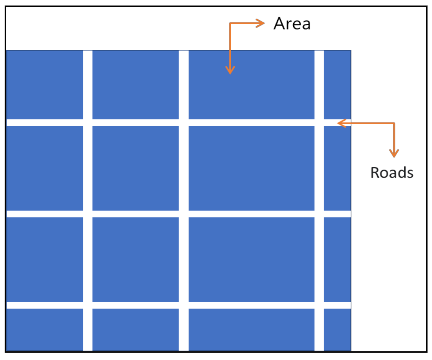
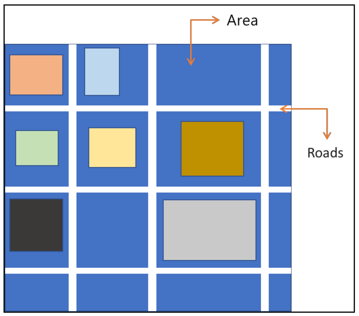
- Color: The colors of the roads and roofs of each building are generally distinct, so use the colors to differentiate them.
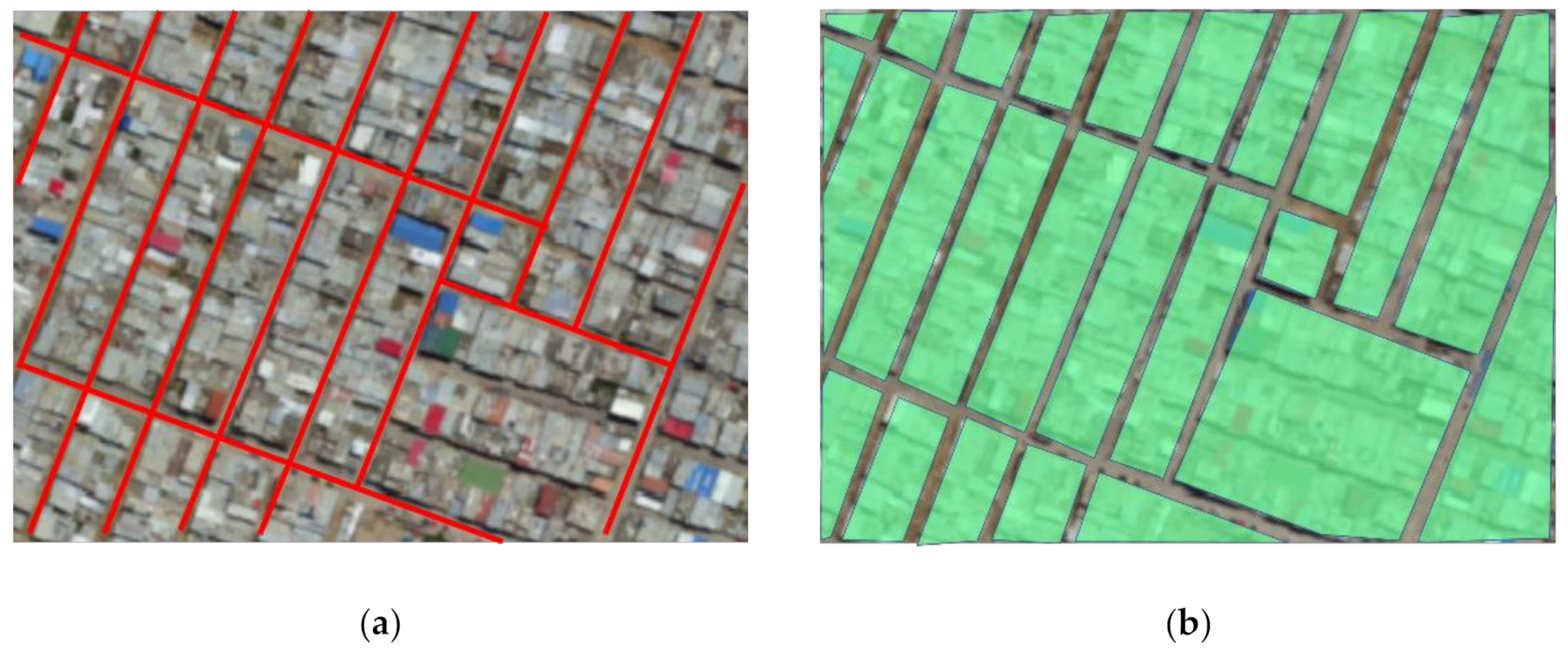
- Road: Use occlusion to classify spaces to ensure that buildings and roads are properly classified.
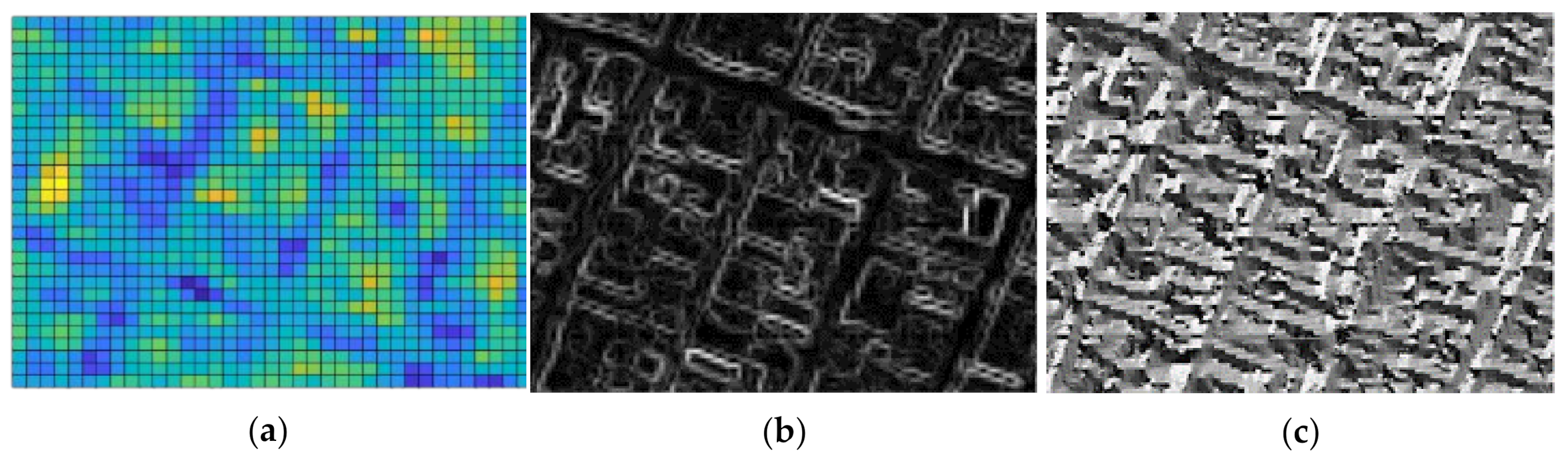
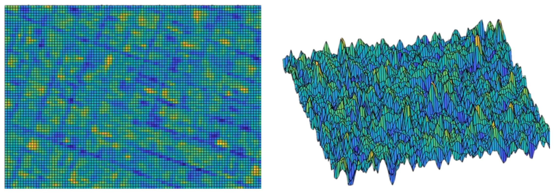
- Stereo: Using the image’s height information, identify the places where the height information varies quickly.
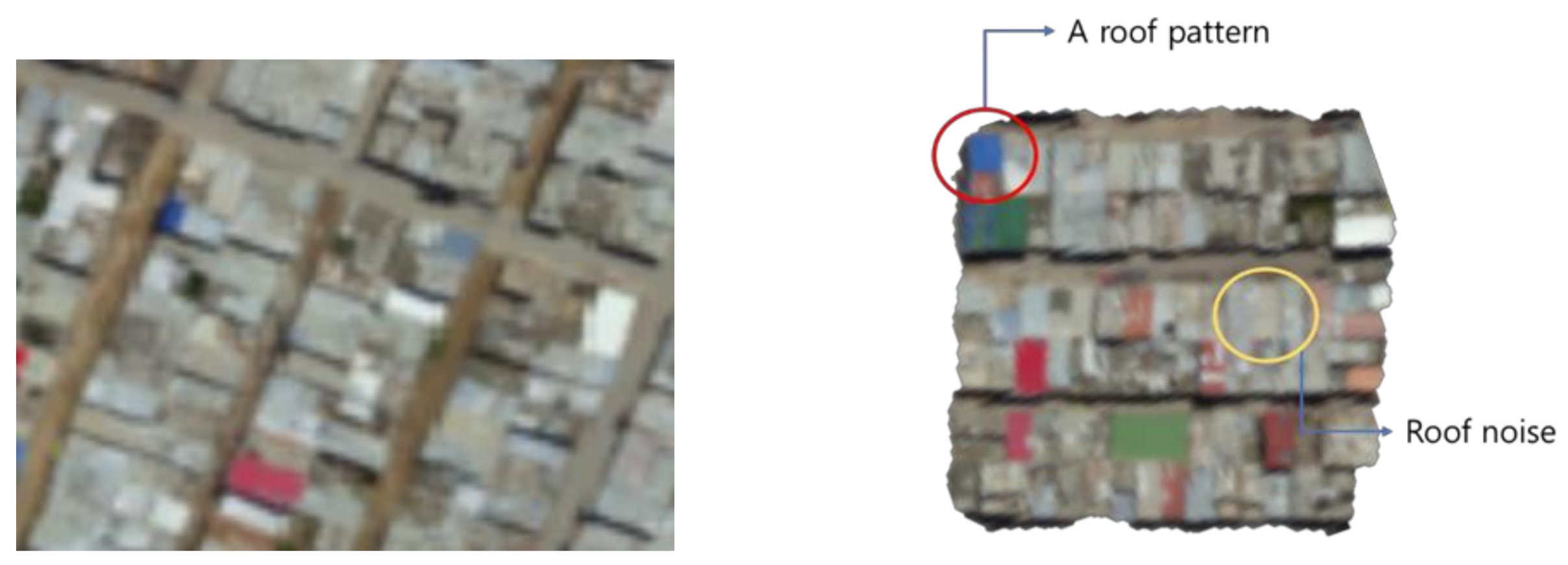
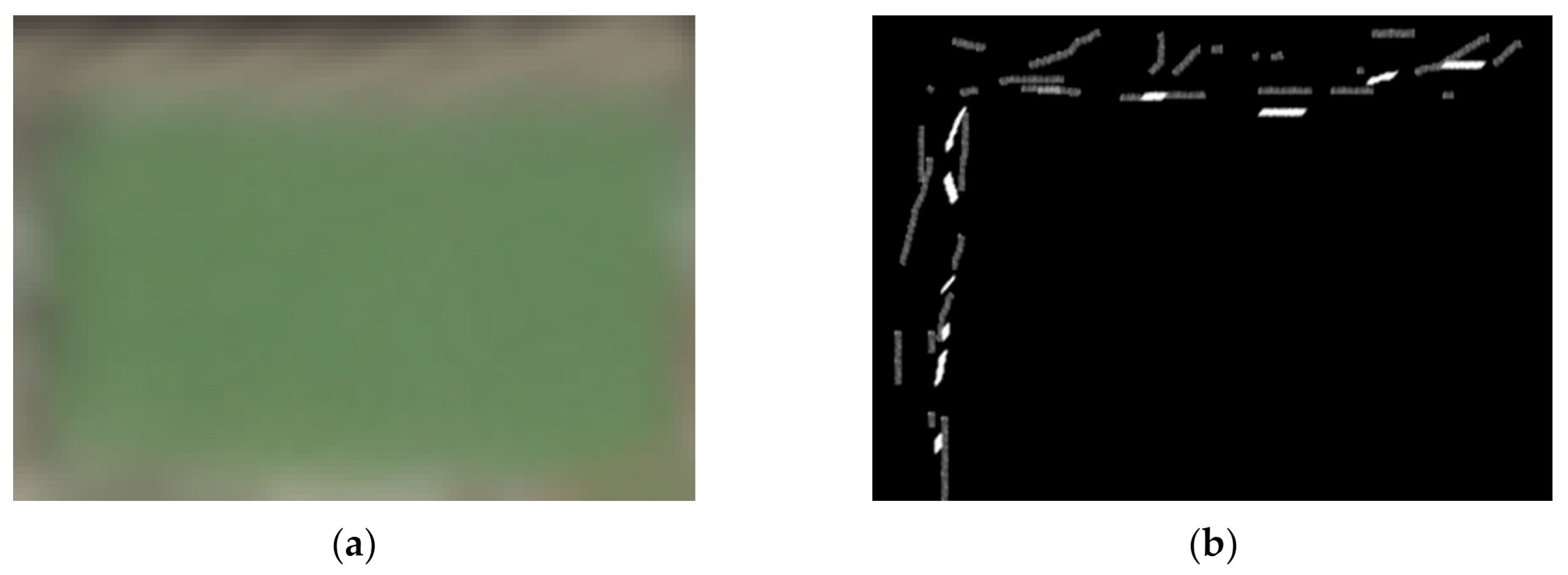
- Noise: Noise in 3D image data is divided into sections where the structure is imperfect or distinctly defined, such as corners, fault lines, and valleys.
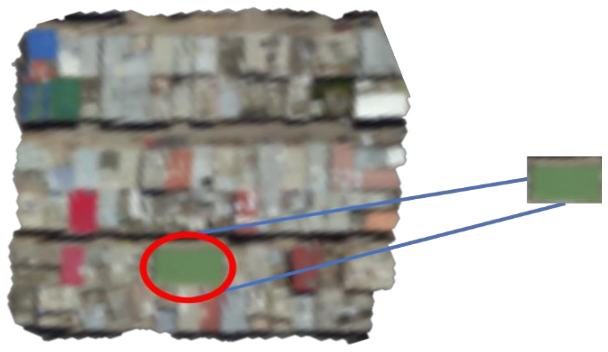
- Pattern: A completed roof will have a specific pattern. It is best to classify using meaningful information such as color, material, and shape, but it is difficult to find these patterns and forms. The shape and color of the roof of the building vary, and even if it is the roof of the same building, the shape and material can be different, causing difficulties in classification.
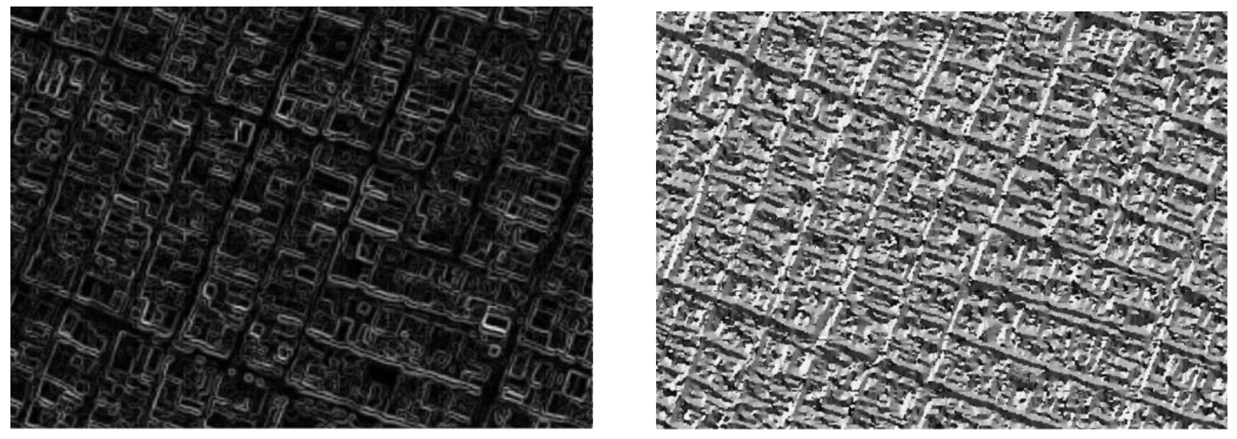
2. Roof Detection Using Image Processing
3. Classification of the Material of the Roof
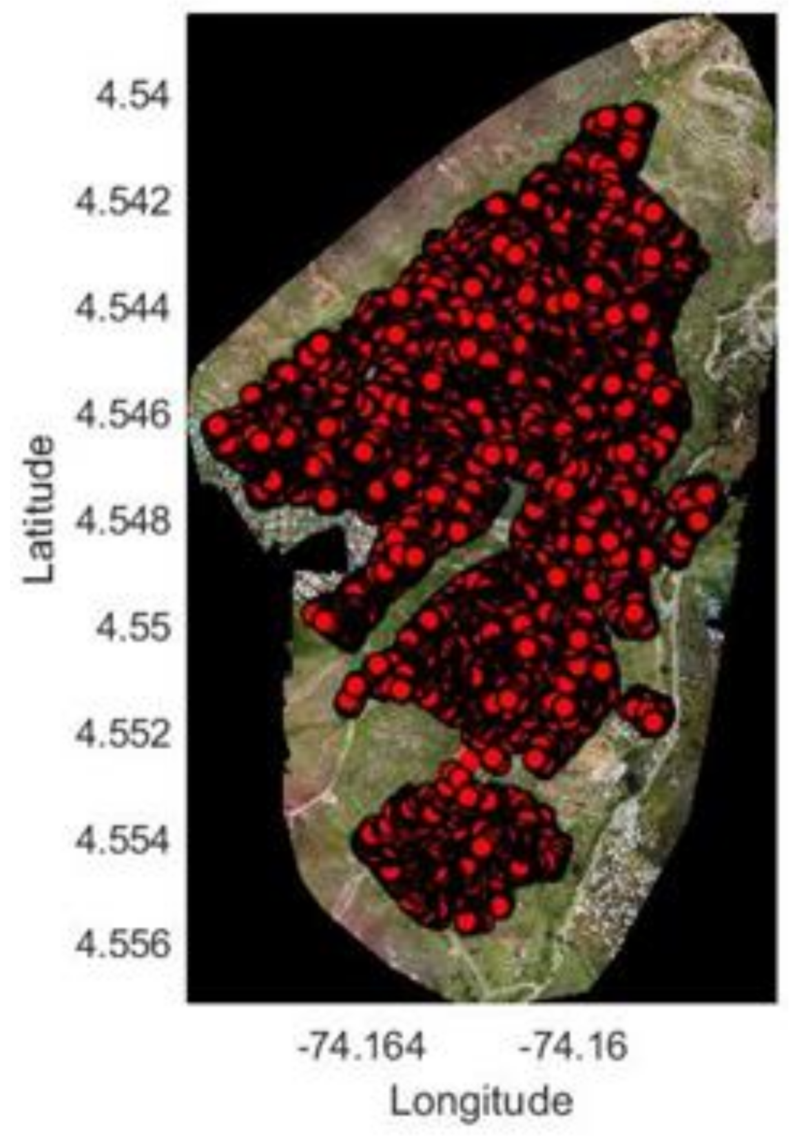
4. Experiment
4.1. Experiment Environment
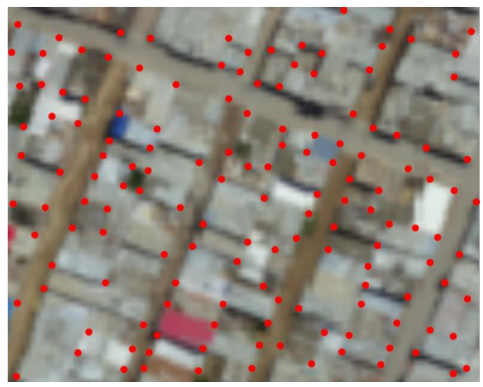
4.2. Detection of Roof Areas
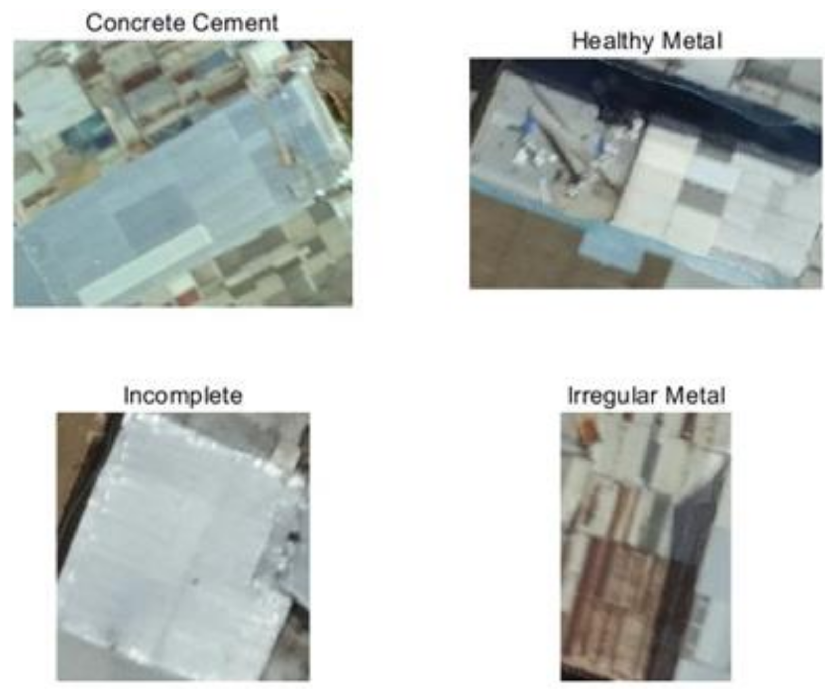
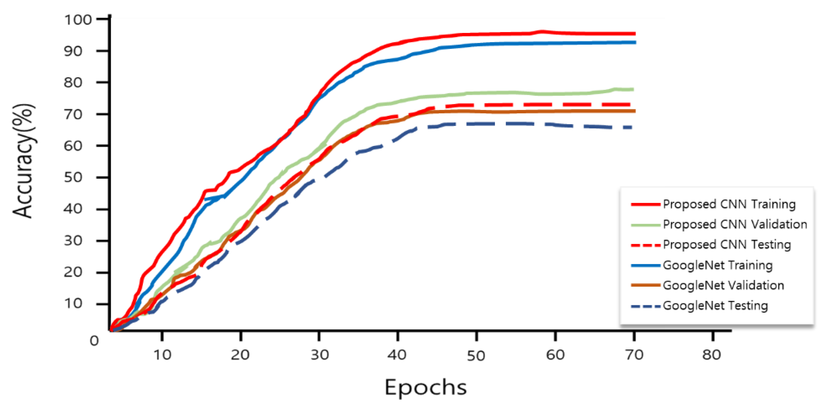
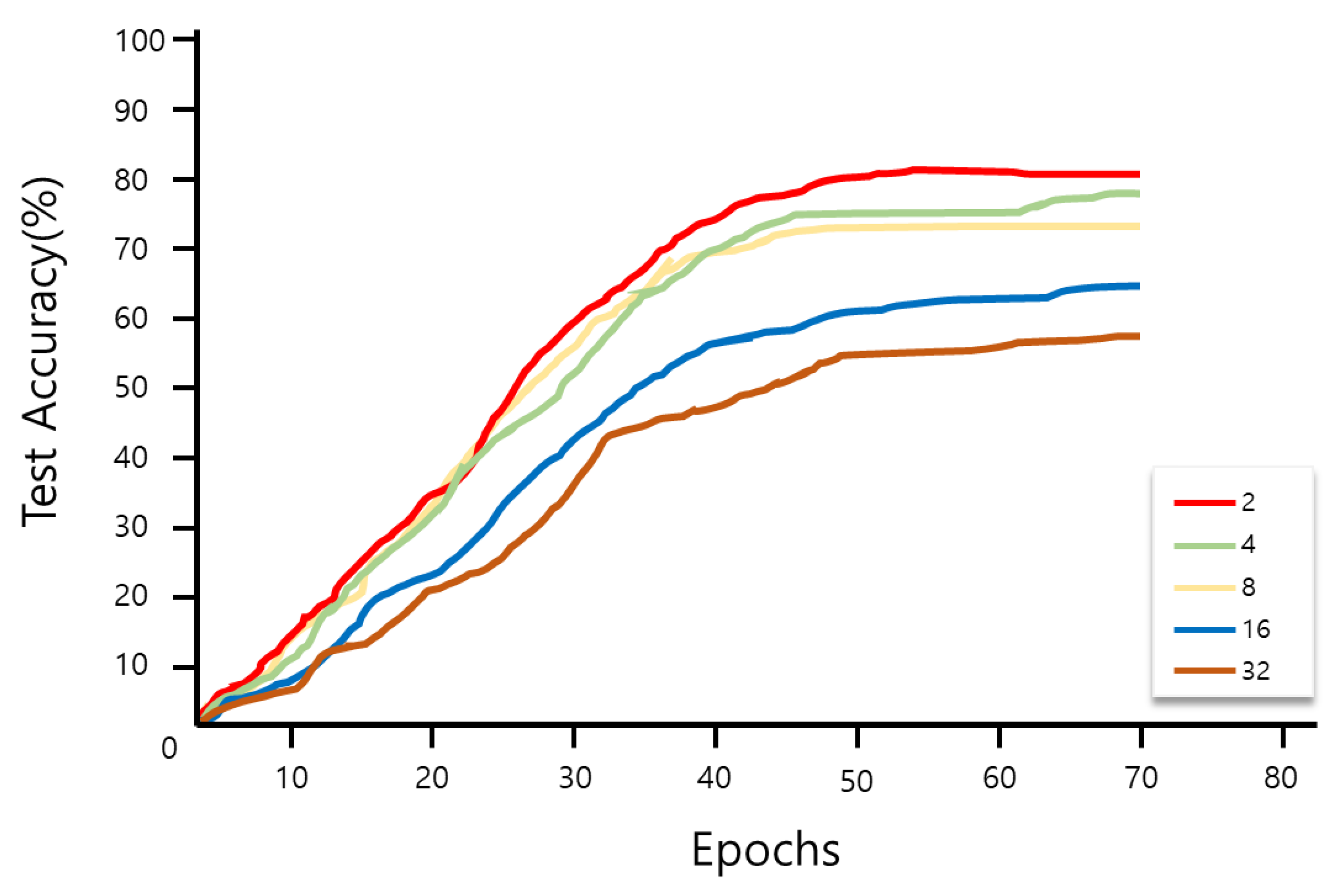
4.3. Roof Material Classification
4.4. Learning for Roof Detection
5. Conclusions
Author Contributions
Funding
Conflicts of Interest
References
- Rajkumar, S.; Malathi, G. A comparative analysis on image quality assessment for real time satellite images. Indian J. Sci. Technol. 2016, 9, 34. [Google Scholar] [CrossRef]
- Ayhan, B.; Kwan, C. Tree, Shrub, and Grass Classification Using Only RGB Images. Remote Sens. 2020, 12, 1333. [Google Scholar] [CrossRef] [Green Version]
- Ayhan, B.; Kwan, C.; Larkin, J.; Kwan, L.; Skarlatos, D.; Vlachos, M. Deep learning model for accurate vegetation classification using RGB image only. Geospatial Informatics X. Int. Soc. Optics Photonics 2020, 11398, 113980H. [Google Scholar]
- Zhao, K.; Kang, J.; Jung, J.; Sohn, G. Building extraction from satellite images using mask R-CNN with building boundary regularization. In Proceedings of the IEEE Conference on Computer Vision and Pattern Recognition Workshops, Salt Lake City, UT, USA, 18–22 June 2018; pp. 247–251. [Google Scholar]
- Dymkova, S.S. Conjunction and synchronization methods of earth satellite images with local cartographic data. In Proceedings of the 2020 Systems of Signals Generating and Processing in the Field of on Board Communications, Moscow, Russia, 19–20 March 2020; IEEE: Piscataway, NJ, USA, 2020; pp. 1–7. [Google Scholar]
- AlMarzooqi, M.; AlNaqbi, A.; AlMheiri, A.; Bezawada, S.; Mohamed, E.A.; Zaki, N. Increase the Exploitation of Mars Satellite Images Via Deep Learning Techniques. In Proceedings of the 2018 International Conference on Robotics, Control and Automation Engineering, Beijing, China, 26–28 December 2018; pp. 171–175. [Google Scholar]
- Torres-Sánchez, J.; López-Granados, F.; Borra-Serrano, I.; Peña, J.M. Assessing UAV-collected image overlap influence on computation time and digital surface model accuracy in olive orchards. Precis. Agric. 2018, 19, 115–133. [Google Scholar] [CrossRef]
- Czyńska, K. High Precision Visibility and Dominance Analysis of Tall Building in Cityscape-on a Basis of Digital Surface Model. In Proceedings of the 36th eCAADe Conference, Lodz, Poland, 17–21 September 2018; pp. 481–488. [Google Scholar]
- Alganci, U.; Besol, B.; Sertel, E. Accuracy assessment of different digital surface models. ISPRS Int. J. Geo-Inf. 2018, 7, 114. [Google Scholar] [CrossRef] [Green Version]
- Yan, Y.; Gao, F.; Deng, S.; Su, N. A hierarchical building segmentation in digital surface models for 3D reconstruction. Sensors 2017, 17, 222. [Google Scholar] [CrossRef] [Green Version]
- Widyaningrum, E.; Lindenbergh, R.C.; Gorte, B.G.H.; Zhou, K. Extraction of building roof edges from LiDAR data o optimize the digital surface model for true orthophoto generation. Int. Arch. Photogramm. Remote Sens. Spat. Inf. Sci. 2018, 42. [Google Scholar] [CrossRef] [Green Version]
- He, X.; Wang, A.; Ghamisi, P.; Li, G.; Chen, Y. LiDAR data classification using spatial transformation and CNN. IEEE Geosci. Remote Sens. Lett. 2018, 16, 125–129. [Google Scholar] [CrossRef]
- Xia, J.; Yokoya, N.; Iwasaki, A. Fusion of hyperspectral and LiDAR data with a novel ensemble classifier. IEEE Geosci. Remote Sens. Lett. 2018, 15, 957–961. [Google Scholar] [CrossRef]
- Wei, Y.; Ding, Z.; Huang, H.; Yan, C.; Huang, J.; Leng, J. A non-contact measurement method of ship block using image-based 3D reconstruction technology. Ocean. Eng. 2019, 178, 463–475. [Google Scholar] [CrossRef]
- Xu, Y.; John, V.; Mita, S.; Tehrani, H.; Ishimaru, K.; Nishino, S. 3D point cloud map based vehicle localization using stereo camera. In Proceedings of the 2017 IEEE Intelligent Vehicles Symposium (IV), Los Angeles, CA, USA, 11–14 June 2017; IEEE: Piscataway, NJ, USA, 2017; pp. 487–492. [Google Scholar]
- Wang, H.; Zhou, M.X.; Zheng, W.Z.; Shi, Z.B.; Li, H.W. 3D machining allowance analysis method for the large thin-walled aerospace component. Int. J. Precis. Eng. Manuf. 2017, 18, 399–406. [Google Scholar] [CrossRef]
- Liu, Y.; Wang, C.; Song, Z.; Wang, M. Efficient global point cloud registration by matching rotation invariant features through translation search. In Proceedings of the European Conference on Computer Vision (ECCV), Munich, Germany, 8–14 September 2018; pp. 448–463. [Google Scholar]
- Muresan, O.; Pop, F.; Gorgan, D.; Cristea, V. Satellite image processing applications in MedioGRID. In Proceedings of the 2006 Fifth International Symposium on Parallel and Distributed Computing, Timisoara, Romania, 6–9 July 2006; IEEE: Piscataway, NJ, USA, 2006; pp. 253–262. [Google Scholar]
- Gorgan, D.; Bacu, V.; Stefanut, T.; Rodila, D.; Mihon, D. Earth Observation application development based on the Grid oriented ESIP satellite image processing platform. Comput. Stand. Interfaces 2012, 34, 541–548. [Google Scholar] [CrossRef]
- Kussul, N.; Shelestov, A.; Skakun, S. Grid system for flood extent extraction from satellite images. Earth Sci. Inform. 2008, 1, 105. [Google Scholar] [CrossRef] [Green Version]
- Chang, N.B.; Bai, K.; Chen, C.F. Smart information reconstruction via time-space-spectrum continuum for cloud removal in satellite images. IEEE J. Sel. Top. Appl. Earth Obs. Remote Sens. 2015, 8, 1898–1912. [Google Scholar] [CrossRef]
- Durand, S.; Malgouyres, F.; Rougé, B. Image deblurring, spectrum interpolation and application to satellite imaging. ESAIM Control Optim. Calc. Var. 2000, 5, 445–475. [Google Scholar] [CrossRef]
- Jianwen, M.; Xiaowen, L.; Xue, C.; Chun, F. Target adjacency effect estimation using ground spectrum measurement and Landsat-5 satellite data. IEEE Trans. Geosci. Remote Sens. 2006, 44, 729–735. [Google Scholar] [CrossRef]
- Sellami, A.; Farah, I.R. Spectra-spatial Graph-based Deep Restricted Boltzmann Networks for Hyperspectral Image Classification. In Proceedings of the 2019 PhotonIcs & Electromagnetics Research Symposium-Spring (PIERS-Spring), Rome, Italy, 17–20 June 2019; IEEE: Piscataway, NJ, USA, 2019; pp. 1055–1062. [Google Scholar]
- Choi, J.; Park, H.; Kim, D.; Choi, S. Unsupervised change detection of KOMPSAT-3 satellite imagery based on cross-sharpened images by Guided filter. Korean J. Remote Sens. 2018, 34, 777–786. [Google Scholar]
- Oh, J.; Lee, C. Epipolar Resampling Module for CAS500 Satellites 3D Stereo Data Processing. Korean J. Remote Sens. 2020, 36, 939–948. [Google Scholar]
- Yuan, B.; Han, L.; Gu, X.; Yan, H. Multi-deep features fusion for high-resolution remote sensing image scene classification. Neural Comput. Appl. 2021, 33, 2047–2063. [Google Scholar] [CrossRef]
- Kashani, A.G.; Graettinger, A.J. Cluster-based roof covering damage detection in ground-based lidar data. Autom. Constr. 2015, 58, 19–27. [Google Scholar] [CrossRef]
- He, M.; Zhu, Q.; Du, Z.; Hu, H.; Ding, Y.; Chen, M. A 3D shape descriptor based on contour clusters for damaged roof detection using airborne LiDAR point clouds. Remote Sens. 2016, 8, 189. [Google Scholar] [CrossRef] [Green Version]
- Sampath, A.; Shan, J. Building roof segmentation and reconstruction from LiDAR point clouds using clustering techniques. Int. Arch. Photogramm. Remote Sens. Spat. Inf. Sci. 2008, 37, 279–284. [Google Scholar]
- Taherzadeh, E.; Shafri, H.Z. Development of a generic model for the detection of roof materials based on an object-based approach using WorldView-2 satellite imagery. Adv. Remote Sens. 2013, 2013. [Google Scholar] [CrossRef] [Green Version]
- Liu, Z.J.; Wang, J.; Liu, W.P. Building extraction from high resolution imagery based on multi-scale object oriented classification and probabilistic Hough transform. In Proceedings of the 2005 IEEE International Geoscience and Remote Sensing Symposium, IGARSS’05, Seoul, Korea, 25–29 July 2005; IEEE: Piscataway, NJ, USA, 2005; pp. 2250–2253. [Google Scholar]
- Beaudoin, N.; Beauchemin, S.S. An accurate discrete Fourier transform for image processing. In Object Recognition Supported by User Interaction for Service Robots; IEEE: Piscataway, NJ, USA, 2002; pp. 935–939. [Google Scholar]


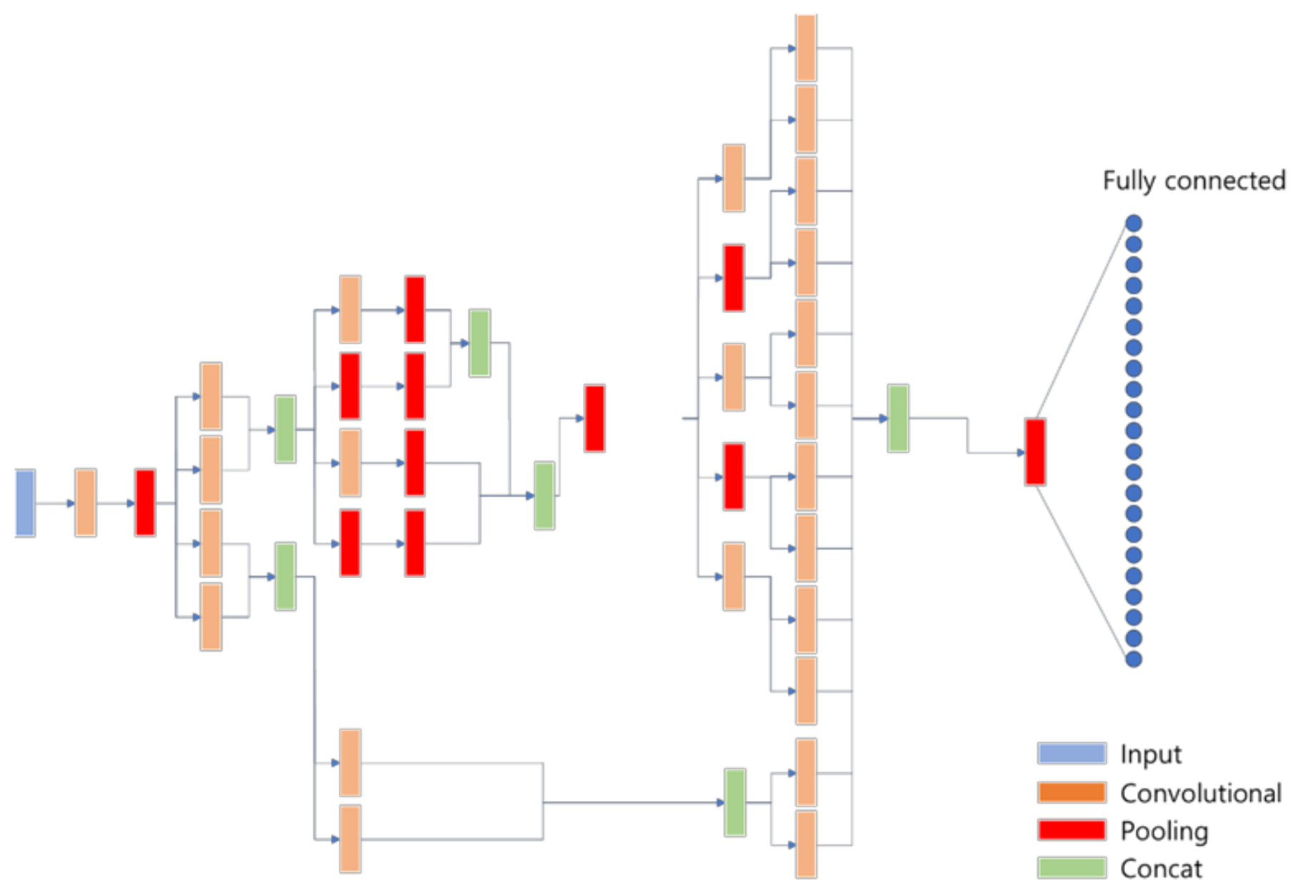
| Layer | Size (Filter, Pool) | Num Filters | Stride | Padding Value | Data Size | Weights Initializer | Bias Initializer |
|---|---|---|---|---|---|---|---|
| Input | 224,224,3 | 224 × 224 × 3 | |||||
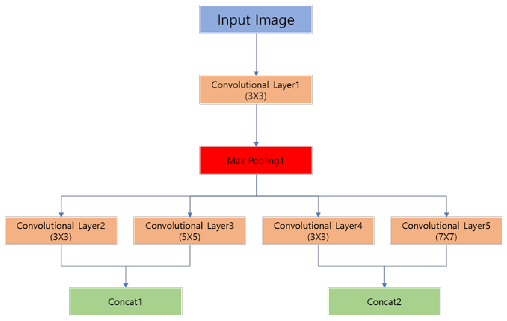
| Conv. Layer1 | 3,3 | 64 | 2,2 | 0 | 112 × 112 × 64 | He | 0 |
| MaxPooling1 | 5,5 | 1,1 | 112 × 112 × 64 | ||||
| Conv. Layer2 | 3,3 | 32 | 2,2 | 0 | 56 × 56 × 32 | He | 0 |
| Conv. Layer3 | 5,5 | 64 | 2,2 | 0 | 56 × 56 × 64 | He | 0 |
| Conv. Layer4 | 3,3 | 64 | 2,2 | 0 | 56 × 56 × 64 | He | 0 |
| Conv. Layer5 | 7,7 | 16 | 2,2 | 0 | 56 × 56 × 16 | He | 0 |
| Concat1 | 56 × 56 × 96 | ||||||
| Concat2 | 56 × 56 × 80 |
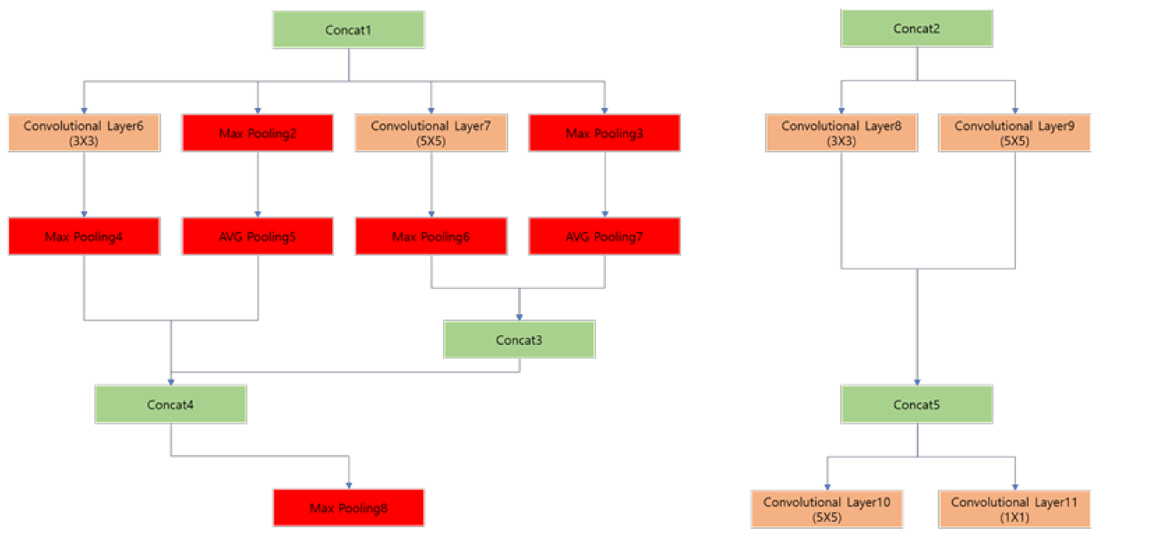
| Layer | Size (Filter, Pool) | Num Filters | Stride | Padding Value | Data Size | Weights Initializer | Bias Initializer |
|---|---|---|---|---|---|---|---|
| Conv. Layer6 | 3,3 | 64 | 1,1 | 0 | 56 × 56 × 64 | He | 0 |
| Max Pooling2 | 5,5 | 1,1 | 56 × 112 × 32 | ||||
| Conv. Layer7 | 5,5 | 32 | 1,1 | 0 | 56 × 56 × 32 | He | 0 |
| Max Pooling3 | 3,3 | 1,1 | 56 × 112 × 32 | ||||
| Max Pooling4 | 3,3 | 2,2 | 28 × 28 × 64 | ||||
| AVG Pooling5 | 3,3 | 2,2 | 28 × 28 × 96 | ||||
| Max Pooling6 | 5,5 | 2,2 | 28 × 28 × 96 | ||||
| AVG Pooling7 | 5,5 | 2,2 | 28 × 28 × 96 | ||||
| Concat3 | 28 × 28 × 128 | ||||||
| Concat4 | 28 × 28 × 288 | ||||||
| Max Pooling8 | 5,5 | 2,2 | 14 × 14 × 288 | ||||
| Conv. Layer8 | 3,3 | 64 | 4,4 | 14 × 14 × 64 | He | 0 | |
| Conv. Layer9 | 5,5 | 32 | 4,4 | 14 × 14 × 32 | He | 0 | |
| Concat5 | 14 × 14 × 96 | ||||||
| Conv. Layer10 | 5,5 | 64 | 2,2 | 7 × 7 × 64 | He | 0 | |
| Conv. Layer11 | 1,1 | 16 | 2,2 | 7 × 7 × 16 | He | 0 |
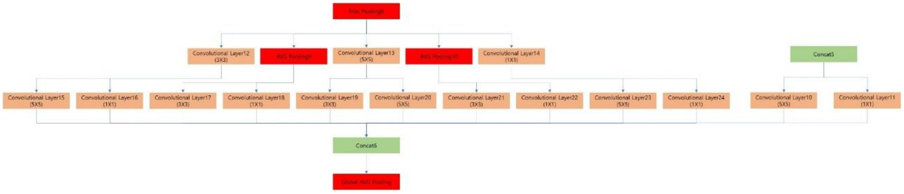
| Layer | Size (Filter, Pool) | Num Filters | Stride | Padding Value | Data Size | Weights Initializer | Bias Initializer |
|---|---|---|---|---|---|---|---|
| Conv. Layer12 | 3,3 | 32 | 1,1 | 0 | 14 × 14 × 32 | He | 0 |
| AVG Pooling9 | 5,5 | 1,1 | 14 × 14 × 288 | ||||
| Conv. Layer13 | 5,5 | 32 | 1,1 | 0 | 14 × 14 × 32 | He | 0 |
| AVG Pooling10 | 3,3 | 1,1 | 14 × 14 × 288 | ||||
| Conv. Layer14 | 1,1 | 32 | 1,1 | 0 | 14 × 14 × 32 | He | 0 |
| Conv. Layer15 | 5,5 | 64 | 2,2 | 0 | 7 × 7 × 64 | He | 0 |
| Conv. Layer16 | 1,1 | 32 | 2,2 | 0 | 7 × 7 × 32 | He | 0 |
| Conv. Layer17 | 3,3 | 128 | 2,2 | 0 | 7 × 7 × 128 | He | 0 |
| Conv. Layer18 | 1,1 | 32 | 2,2 | 0 | 7 × 7 × 32 | He | 0 |
| Conv. Layer19 | 3,3 | 32 | 2,2 | 0 | 7 × 7 × 32 | He | 0 |
| Conv. Layer20 | 5,5 | 64 | 2,2 | 0 | 7 × 7 × 64 | He | 0 |
| Conv. Layer21 | 3,3 | 64 | 2,2 | 0 | 7 × 7 × 64 | He | 0 |
| Conv. Layer22 | 1,1 | 16 | 2,2 | 0 | 7 × 7 × 16 | He | 0 |
| Conv. Layer23 | 5,5 | 64 | 2,2 | 0 | 7 × 7 × 64 | He | 0 |
| Conv. Layer24 | 1,1 | 16 | 2,2 | 0 | 7 × 7 × 16 | He | 0 |
| Concat6 | 7 × 7 × 592 | ||||||
| Global AVGPooling | 7,7 | 1 × 1 × 592 |
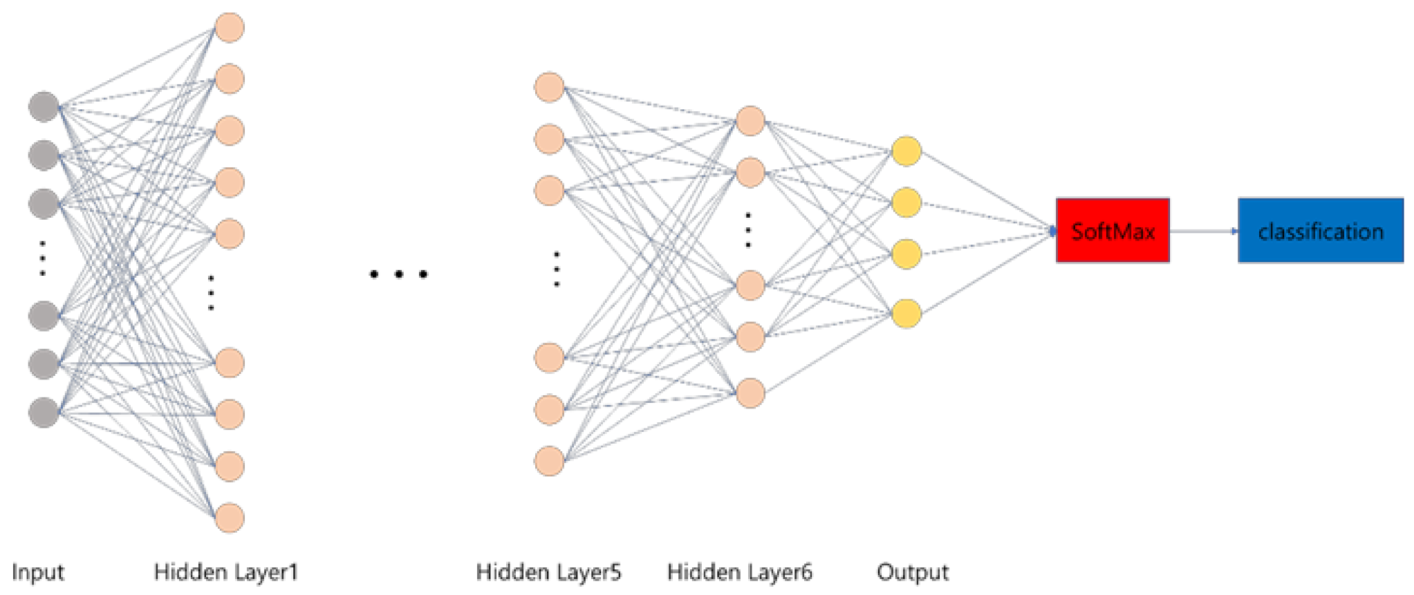
| Hidden Layer | 6 |
| Hidden Layer 1 Node | 900 |
| Hidden Layer 2 Node | 1200 |
| Hidden Layer 3 Node | 600 |
| Hidden Layer 4 Node | 200 |
| Hidden Layer 5 Node | 50 |
| Hidden Layer 6 Node | 10 |
| Dropout | 50% |
| Weight Initialization | He Method |
| Active Function | Relu |
| Batch Size | 8 |
| Number of Epochs | 70 |
| Training Accuracy | Validation Accuracy | Testing Accuracy | |
|---|---|---|---|
| Proposed CNN | 97.4% ± 0.54% | 78.7% ± 0.95% | 73.3% ± 1.002% |
| GoogleNet | 92.5% ± 0.72% | 71.3% ± 0.84% | 68.6% ± 1.16% |
| Concrete Cement | Healthy Metal | Incomplete | Irregular Metal | ||
|---|---|---|---|---|---|
| Proposed CNN | Training Accuracy | 98.7% | 97.5% | 96.7% | 94.1% |
| Validation Accuracy | 83.4% | 80.3% | 77.2% | 76.0% | |
| Testing Accuracy | 77.8% | 74.6% | 72.1% | 70.3% | |
| GoogleNet | Training Accuracy | 95.6% | 94.2% | 91.1% | 90.6% |
| Validation Accuracy | 74.5% | 73.4% | 70.6% | 68.3% | |
| Testing Accuracy | 70.3% | 70.1% | 66.7% | 65.1% | |
| Precision | Recall | F1 Score | |
|---|---|---|---|
| Proposed CNN | 0.97 | 0.87 | 0.91 |
| GoogleNet | 0.96 | 0.81 | 0.87 |
| Epochs: 50 | Epochs: 60 | Epochs: 70 | Epochs: 80 | Epochs: 90 | |
|---|---|---|---|---|---|
| Proposed CNN | 71.8% ± 1.61% | 73.1% ± 1.2% | 73.3% ± 1.002% | 73.5% ± 0.78% | 73.3% ± 0.77% |
| GoogleNet | 67.6% ± 1.66% | 68.5% ± 1.25% | 68.6% ± 1.16% | 68.3% ± 0.94% | 68.5% ± 0.95% |
Publisher’s Note: MDPI stays neutral with regard to jurisdictional claims in published maps and institutional affiliations. |
© 2021 by the authors. Licensee MDPI, Basel, Switzerland. This article is an open access article distributed under the terms and conditions of the Creative Commons Attribution (CC BY) license (https://creativecommons.org/licenses/by/4.0/).
Share and Cite
Kim, J.; Bae, H.; Kang, H.; Lee, S.G. CNN Algorithm for Roof Detection and Material Classification in Satellite Images. Electronics 2021, 10, 1592. https://doi.org/10.3390/electronics10131592
Kim J, Bae H, Kang H, Lee SG. CNN Algorithm for Roof Detection and Material Classification in Satellite Images. Electronics. 2021; 10(13):1592. https://doi.org/10.3390/electronics10131592
Chicago/Turabian StyleKim, Jonguk, Hyansu Bae, Hyunwoo Kang, and Suk Gyu Lee. 2021. "CNN Algorithm for Roof Detection and Material Classification in Satellite Images" Electronics 10, no. 13: 1592. https://doi.org/10.3390/electronics10131592