1. Introduction
Decision trees are used in many areas of computer science as a means for knowledge representation, as classifiers, and as algorithms to solve different problems of combinatorial optimization, computational geometry, etc. [
1,
2,
3]. They are studied, in particular, in test theory initiated by Chegis and Yablonskii [
4], rough set theory initiated by Pawlak [
5,
6,
7], and exact learning initiated by Angluin [
8,
9]. These theories are closely related: attributes from rough set theory and test theory correspond to membership queries from exact learning. Exact learning studies additionally the so-called equivalence queries. The notion of “minimally adequate teacher” that allows both membership and equivalence queries was discussed by Angluin in Reference [
10]. Relations between exact learning and PAC learning proposed by Valiant [
11] are discussed in Reference [
8].
In this paper, which is an extension of two conference papers [
12,
13], we add the notion of a hypothesis to the model that has been considered in rough set theory, as well as in test theory. This model allows us to use an analog of equivalence queries. Our goal is to check whether it is possible to reduce the time and space complexity of decision trees if we use additionally hypotheses. Decision trees with less complexity are more understandable and more suitable as a means for knowledge representation. Note that, to improve the understandability, we should not only try to minimize the number of nodes in a decision tree but also its depth that is the unimprovable upper bound on the number of conditions describing objects accepted by a path from the root to a terminal node of the tree. In this paper, we concentrate only on the consideration of complexity of decision trees and do not study many recent problems considered in machine learning [
14,
15,
16,
17].
Let T be a decision table with n conditional attributes having values from the set in which rows are pairwise different, and each row is labeled with a decision from . For a given row of T, we should recognize the decision attached to this row. To this end, we can use decision trees based on two types of queries. We can ask about the value of an attribute on the given row. We will obtain an answer of the kind , where is the number in the intersection of the given row and the column . We can also ask if a hypothesis is true, where are numbers from the columns , respectively. Either this hypothesis will be confirmed or we obtain a counterexample in the form , where , and is a number from the column different from . The considered hypothesis is called proper if is a row of the table T.
In this paper, we study four cost functions that characterize the complexity of decision trees: the depth, the number of realizable nodes relative to T, the number of realizable terminal nodes relative to T, and the number of working nodes. We consider the depth of a decision tree as its time complexity, which is equal to the maximum number of queries in a path from the root to a terminal node of the tree. The remaining three cost functions characterize the space complexity of decision trees. A node is called realizable relative to T if, for a row of T and some choice of counterexamples, the computation in the tree will pass through this node. Note that, in the considered trees, all working nodes are realizable.
Decision trees using hypotheses can be essentially more efficient than the decision trees using only attributes. Let us consider an example, the problem of computation of the conjunction . The minimum depth of a decision tree solving this problem using the attributes is equal to n. The minimum number of realizable nodes in such decision trees is equal to , the minimum number of working nodes is equal to n, and the minimum number of realizable terminal nodes is equal to . However, the minimum depth of a decision tree solving this problem using proper hypotheses is equal to 1: it is enough to ask only about the hypothesis . If it is true, then the considered conjunction is equal to 1. Otherwise, it is equal to 0. The obtained decision tree contains one working node and realizable terminal nodes, altogether realizable nodes.
We study the following five types of decision trees:
Decision trees that use only attributes.
Decision trees that use only hypotheses.
Decision trees that use both attributes and hypotheses.
Decision trees that use only proper hypotheses.
Decision trees that use both attributes and proper hypotheses.
For each cost function, we propose a dynamic programming algorithm that, for a given decision table and given type of decision trees, finds the minimum cost of a decision tree of the considered type for this table. Note that dynamic programming algorithms for the optimization of decision trees of the type 1 were studied in Reference [
18] for decision tables with one-valued decisions and in Reference [
19] for decision tables with many-valued decisions. The dynamic programming algorithms for the optimization of decision trees of all five types were studied in References [
12,
13] for the depth and for the number of realizable nodes.
It is interesting to consider not only specially chosen examples as the conjunction of
n variables. For each cost function, we compute the minimum cost of a decision tree for each of the considered five types for eight decision tables from the UCI ML Repository [
20]. We do the same for randomly generated Boolean functions with
n variables, where
.
From the obtained experimental results, it follows that, generally, the decision trees of the types 3 and 5 have less complexity than the decision trees of the type 1. Therefore, such decision trees can be useful as a means for knowledge representation. Decision trees of the types 2 and 4 have, generally, too many nodes.
Based on the experimental results, we formulate and prove the following hypothesis: for any decision table, we can construct a decision tree with the minimum number of realizable terminal nodes using only attributes.
The motivation for the work is related to the use of decision trees to represent knowledge: we try to reduce the complexity of decision trees (and improve their understandability) by using hypotheses. The main achievements of the work are the following: (i) we have proposed dynamic programming algorithms for optimizing five types of decision trees relative to four cost functions, and (ii) we have shown cases, when the use of hypotheses leads to the decrease in the complexity of decision trees.
2. Decision Tables
A decision table is a table T with columns filled with numbers from the set . Columns of this table are labeled with conditional attributes . Rows of the table are pairwise different. Each row is labeled with a number from that is interpreted as a decision. Rows of the table are interpreted as tuples of values of the conditional attributes.
Each decision table can be represented by a word (sequence) over the alphabet : numbers from are in binary representation, we use the symbol “;” to separate two numbers from , and we use the symbol “|” to separate two rows (for each row, we add corresponding decision as the last number in the row). The length of this word is called the size of the decision table.
A decision table T is called empty if it has no rows. The table T is called degenerate if it is empty or all rows of T are labeled with the same decision.
We denote and denote by the set of decisions attached to the rows of T. For any conditional attribute , we denote by the set of values of the attribute in the table T. We denote by the set of conditional attributes of T for which .
A system of equations over
T is an arbitrary equation system of the kind
where
,
, and
(if
, then the considered equation system is empty).
Let T be a nonempty table. A subtable of T is a table obtained from T by removal of some rows. We correspond to each equation system S over T a subtable of the table T. If the system S is empty, then . Let S be nonempty and . Then, is the subtable of the table T containing the rows from T that, in the intersection with columns, have numbers , respectively. Such nonempty subtables, including the table T, are called separable subtables of T. We denote by the set of separable subtables of the table T.
3. Decision Trees
Let T be a nonempty decision table with n conditional attributes . We consider the decision trees with two types of queries. We can choose an attribute and ask about its value. This query has the set of answers . We can formulate a hypothesis over T in the form of , where , and ask about this hypothesis. This query has the set of answers . The answer H means that the hypothesis is true. Other answers are counterexamples. The hypothesis H is called proper for T if is a row of the table T.
A decision tree over T is a marked finite directed tree with the root in which:
Each terminal node is labeled with a number from the set .
Each node, which is not terminal (such nodes are called working), is labeled with an attribute from the set or with a hypothesis over T.
If a working node is labeled with an attribute from , then, for each answer from the set , there is exactly one edge labeled with this answer, which leave this node and there are no any other edges leaving this node.
If a working node is labeled with a hypothesis over T, then, for each answer from the set , there is exactly one edge labeled with this answer, which leaves this node and there are no any other edges leaving this node.
Let be a decision tree over T and v be a node of . We now define an equation system over T associated with the node v. We denote by the directed path from the root of to the node v. If there are no working nodes in , then is the empty system. Otherwise, is the union of equation systems attached to the edges of the path .
A decision tree over T is called a decision tree for T if, for any node v of ,
The node v is terminal if and only if the subtable is degenerate.
If v is a terminal node and the subtable is empty, then the node v is labeled with the decision 0.
If v is a terminal node and the subtable is nonempty, then the node v is labeled with the decision attached to all rows of .
A complete path in is an arbitrary directed path from the root to a terminal node in . As the time complexity of a decision tree, we consider its depth that is the maximum number of working nodes in a complete path in the tree or, which is the same, the maximum length of a complete path in the tree. We denote by the depth of a decision tree .
As the space complexity of the decision tree , we consider the number of its realizable relative to T nodes. A node v of is called realizable relative to T if and only if the subtable is nonempty. We denote by the number of nodes in that are realizable relative to T. We also consider two more cost functions relative to the space complexity: — the number of terminal nodes in that are realizable relative to T and — the number of working nodes in . Note that all working nodes of are realizable relative to T.
We will use the following notation:
For , is the minimum depth of a decision tree of the type k for T.
For , is the minimum number of nodes realizable relative to T in a decision tree of the type k for T.
For , is the minimum number of terminal nodes realizable relative to T in a decision tree of the type k for T.
For , is the minimum number of working nodes in a decision tree of the type k for T.
4. Construction of Directed Acyclic Graph
Let
T be a nonempty decision table with
n conditional attributes
. We now describe an Algorithm
for the construction of a directed acyclic graph (DAG)
that will be used for the study of decision trees. Nodes of this graph are separable subtables of the table
T. During each iteration we process one node. We start with the graph that consists of one node
T, which is not processed and finish when all nodes of the graph are processed. This algorithm can be considered as a special case of the algorithm for DAG construction considered in Reference [
18].
| Algorithm (construction of DAG ). |
| Input: A nonempty decision table T with n conditional attributes . |
| Output: Directed acyclic graph . |
Construct the graph that consists of one node T, which is not marked as processed. If all nodes of the graph are processed, then the algorithm halts and returns the resulting graph as . Otherwise, choose a node (table) that has not been processed yet. If is degenerate, then mark the node as processed and proceed to step 2. If is not degenerate, then, for each , draw a bundle of edges from the node . Let . Then, draw k edges from and label these edges with systems of equations . These edges enter nodes , respectively. If some of the nodes are not present in the graph, then add these nodes to the graph. Mark the node as processed and return to step 2.
|
The following statement about time complexity of the Algorithm
follows immediately from Proposition 3.3 [
18].
Proposition 1. The time complexity of the Algorithm is bounded from above by a polynomial on the size of the input table T and the number of different separable subtables of T.
Generally, the time complexity of the Algorithm
is exponential, depending on the size of the input decision tables. Note that, in Section 3.4 of the book [
18], classes of decision tables are described for each of which the number of separable subtables of decision tables from the class is bounded from above by a polynomial on the number of columns in the tables. For each of these classes, the time complexity of the Algorithm
is polynomial depending on the size of the input decision tables.
Note that similar results can be obtained for the space complexity of the considered algorithm.
5. Minimizing the Depth
In this section, we consider some results obtained in Reference [
12]. Let
T be a nonempty decision table with
n conditional attributes
. We can use the DAG
to compute values
. Let
. To find the value
, for each node
of the DAG
, we compute the value
. It will be convenient for us to consider not only subtables that are nodes of
but also empty subtable
of
T and subtables
that contain only one row
r of
T and are not nodes of
. We begin with these special subtables and terminal nodes of
(nodes without leaving edges) that are degenerate separable subtables of
T and step-by-step move to the table
T.
Let be a terminal node of or for some row r of T. Then, : the decision tree that contains only one node labeled with the decision attached to all rows of is a decision tree for . If , then : the decision tree that contains only one node labeled with 0 will be considered as a decision tree for .
Let be a nonterminal node of such that, for each child of , we already know the value . Based on this information, we can find the minimum depth of a decision tree for , which uses for the subtables corresponding to the children of the root decision trees of the type k and in which the root is labeled:
With an attribute from (we denote by the minimum depth of such a decision tree).
With a hypothesis over T (we denote by the minimum depth of such a decision tree).
With a proper hypothesis over T (we denote by the minimum depth of such a decision tree).
Since is nondegenerate, the set is nonempty. We now describe three procedures for computing the values , , and , respectively.
Let us consider a decision tree
for
in which the root is labeled with an attribute
. For each
, there is an edge that leaves the root and enters a node
. This edge is labeled with the equation system
. The node
is the root of a decision tree of the type
k for
for which the depth is equal to
. It is clear that
Since
for any
,
Evidently, for any , the subtable is a child of in the DAG , i.e., we know the value .
One can show that is the minimum depth of a decision tree for in which the root is labeled with the attribute and which uses for the subtables corresponding to the children of the root decision trees of the type k.
We should not consider attributes
since, for each such attribute, there is
with
, i.e., based on this attribute, we cannot construct an optimal decision tree for
. As a result, we have
Computation of . Construct the set of attributes
. For each attribute
, compute the value
using (
1). Compute the value
using (
2).
Remark 2. Let Θ be a nonterminal node of the DAG such that, for each child of Θ, we already know the value . Then, the procedure of computation of the value has polynomial time complexity depending on the size of decision table T.
A hypothesis over T is called admissible for and an attribute if, for any , . The hypothesis H is not admissible for and an attribute if and only if and . The hypothesis H is called admissible for if it is admissible for and any attribute .
Let us consider a decision tree
for
in which the root is labeled with an admissible for
hypothesis
. The set of answers for the query corresponding to the hypothesis
H is equal to
. For each
, there is an edge that leaves the root of
and enters a node
. This edge is labeled with the equation system
S. The node
is the root of a decision tree of the type
k for
, which depth is equal to
. It is clear that
We have
or
for some row
r of
T. Therefore,
. Since
H is admissible for
,
for any attribute
. It is clear that
and
for any attribute
and any
such that
. Therefore,
It is clear that, for any
and any
, the subtable
is a child of
in the DAG
, i.e., we know the value
.
One can show that is the minimum depth of a decision tree for in which the root is labeled with the hypothesis H and which uses for the subtables corresponding to the children of the root decision trees of the type k.
We should not consider hypotheses that are not admissible for since, for each such hypothesis H for corresponding query, there is an answer with , i.e., based on this hypothesis, we cannot construct an optimal decision tree for .
Computation of. First, we construct a hypothesis:
for
. Let
. Then,
is equal to the only number in the set
. Let
. Then,
is the minimum number from
for which
. It is clear that
is admissible for
. Compute the value
using (
3). Simple analysis of (
3) shows that
.
Remark 3. Let Θ be a nonterminal node of the DAG such that, for each child of Θ, we already know the value . Then, the procedure of computation of the value has polynomial time complexity depending on the size of decision table T.
Computation of. For each row
of the decision table
T, we check if the corresponding proper hypothesis
is admissible for
. For each admissible for
proper hypothesis
, we compute the value
using (
3). One can show that the minimum among the obtained numbers is equal to
.
Remark 4. Let Θ be a nonterminal node of the DAG such that, for each child of Θ, we already know the value . Then, the procedure of computation of the value has polynomial time complexity depending on the size of decision table T.
We describe an Algorithm that, for a given nonempty decision table T and given , calculates the value , which is the minimum depth of a decision tree of the type k for the table T. During the work of this algorithm, we find for each node of the DAG the value .
| Algorithm (computation of ). |
| Input: A nonempty decision table T, the directed acyclic graph , and number . |
| Output: The value . |
If a number is attached to each node of the DAG , then return the number attached to the node T as and halt the algorithm. Otherwise, choose a node of the graph without attached number, which is either a terminal node of or a nonterminal node of for which all children have attached numbers. If is a terminal node, then attach to it the number and proceed to step 1. If is not a terminal node, then, depending on the value k, do the following: In the case , compute the value and attach to the value . In the case , compute the value and attach to the value . In the case , compute the values and , and attach to the value . In the case , compute the value and attach to the value . In the case , compute the values and , and attach to the value .
Proceed to step 1.
|
Using Remarks 2–4, one can prove the following statement.
Proposition 5. The time complexity of the Algorithm is bounded from above by a polynomial on the size of the input table T and the number of different separable subtables of T.
A similar bound can be obtained for the space complexity of the considered algorithm.
6. Minimizing the Number of Realizable Nodes
In this section, we consider some results obtained in Reference [
13]. Let
T be a nonempty decision table with
n conditional attributes
. We can use the DAG
to compute values
. Let
. To find the value
, we compute the value
for each node
of the DAG
. We will consider not only subtables that are nodes of
but also empty subtable
of
T and subtables
that contain only one row
r of
T and are not nodes of
. We begin with these special subtables and terminal nodes of
(nodes without leaving edges) that are degenerate separable subtables of
T and step-by-step move to the table
T.
Let be a terminal node of or for some row r of T. Then, : the decision tree that contains only one node labeled with the decision attached to all rows of is a decision tree for . The only node of this tree is realizable relative to . If , then : the decision tree that contains only one node labeled with 0 will be considered as a decision tree for . The only node of this tree is not realizable relative to .
Let be a nonterminal node of such that, for each child of , we already know the value . Based on this information, we can find the minimum number of realizable relative to nodes in a decision tree for , which uses for the subtables corresponding to the children of the root decision trees of the type k and in which the root is labeled
With an attribute from (we denote by the minimum number of realizable relative to nodes in such a decision tree).
With a hypothesis over T (we denote by the minimum number of realizable relative to nodes in such a decision tree).
With a proper hypothesis over T (we denote by the minimum number of realizable relative to nodes in such a decision tree).
We now describe three procedures for computing the values , , and , respectively. Since is nondegenerate, the set is nonempty.
Let us consider a decision tree
for
in which the root is labeled with an attribute
. For each
, there is an edge that leaves the root and enters a node
. This edge is labeled with the equation system
. The node
is the root of a decision tree of the type
k for
for which the number of realizable relative to
nodes is equal to
. It is clear that
. Since
for any
,
Evidently, for any , the subtable is a child of in the DAG , i.e., we know the value . One can show that is the minimum number of realizable relative to nodes in a decision tree for , which uses for the subtables corresponding to the children of the root decision trees of the type k and in which the root is labeled with the attribute .
We should not consider attributes
since, for each such attribute, there is
with
, i.e., based on this attribute, we cannot construct an optimal decision tree for
. As a result, we have
Computation of. Construct the set of attributes
. For each attribute
, compute the value
using (
4). Compute the value
using (
5).
Let us consider a decision tree for in which the root is labeled with an admissible for hypothesis . For each , there is an edge that leaves the root of and enters a node . This edge is labeled with the equation system S. The node is the root of a decision tree of the type k for , for which the number of realizable relative to nodes is equal to . It is clear that .
Denote
. It is easy to show that
if
r is not a row of
and
if
r is a row of
. Therefore,
Since
H is admissible for
,
for any attribute
. It is clear that
and
for any attribute
and any
such that
. Therefore,
where
Evidently, for any and any , the subtable is a child of in the DAG , i.e., we know the value . It is easy to show that is the minimum number of realizable relative to nodes in a decision tree for , which uses for the subtables corresponding to the children of the root decision trees of the type k and in which the root is labeled with the admissible for hypothesis H.
We should not consider hypotheses that are not admissible for
since, for each such hypothesis
H for corresponding query, there is an answer
with
, i.e., based on this hypothesis, we cannot construct an optimal decision tree for
. As a result, we have
where
is the set of admissible hypotheses for
.
For each
, denote
and
. Set
. It is clear that, for each
, the hypothesis
is admissible for
. Simple analysis of (
8) shows that the set
coincides with the set of admissible for
hypotheses
H that minimize the value
. Denote
, where
.
Let there be a tuple
, which is not a row of
. Then,
and
. Let all tuples from
be rows of
. We now show that
. For any
, we have
. Therefore,
. Let us assume that
. Then, by (
9), there exists an admissible for
hypothesis
for which
and
, but this is impossible since, according to (
7),
.
As a result, we have if not all tuples from are rows of , and if all tuples from are rows of .
Computation of. For each
, we compute the value:
and construct the set
. For a tuple
, using (
8), we compute the value
. Then, we count the number
N of rows from
that belong to the set
and compute the cardinality
of the set
that is equal to
. As a result, we have
if
and
if
.
Computation of. For each row
of the decision table
T, we check if the corresponding proper hypothesis
is admissible for
. For each admissible for
proper hypothesis
, we compute the value
using (
6), (
7), and (
8). One can show that the minimum among the obtained numbers is equal to
.
We now consider an algorithm that, for a given nonempty decision table T and number , calculates the value , which is the minimum number of nodes realizable relative to T in a decision tree of the type k for the table T. During the work of this algorithm, we find for each node of the DAG the value .
The description of the algorithm is similar to the description of the Algorithm . Instead of , we should use . For each , instead of , we should use . In particular, for each terminal node , .
One can show that the procedures of computation of the values , , and have polynomial time complexity depending on the size of the decision table T. Using this fact, one can prove the following statement.
Proposition 6. The time complexity of the algorithm is bounded from above by a polynomial on the size of the input table T and the number of different separable subtables of T.
A similar bound can be obtained for the space complexity of the considered algorithm.
7. Minimizing the Number of Realizable Terminal Nodes
The procedure considered in this section is similar to the procedure of the minimization of the number of realizable nodes. The main difference is that, in decision trees with the minimum number of realizable terminal nodes, it is possible to meet constant attributes and hypotheses that are not admissible. Fortunately, for any decision table and any type of decision trees, there is a decision tree of this type with the minimum number of realizable terminal nodes for the considered table that do not use such attributes and hypotheses. We will omit many details and describe main steps only.
Let T be a nonempty decision table with n conditional attributes and . To find the value , we compute the value for each node of the DAG . We begin with terminal nodes of that are degenerate separable subtables of T and step-by-step move to the table T.
Let be a terminal node of . Then, : the decision tree that contains only one node labeled with the decision attached to all rows of is a decision tree for . The only node of this tree is a terminal node realizable relative to .
Let be a nonterminal node of such that, for each child of , we already know the value . Based on this information, we can find the minimum number of realizable relative to terminal nodes in a decision tree for , which uses for the subtables corresponding to children of the root decision trees of the type k and in which the root is labeled
With an attribute from (we denote by the minimum number of realizable relative to terminal nodes in such a decision tree).
With a hypothesis over T (we denote by the minimum number of realizable relative to terminal nodes in such a decision tree).
With a proper hypothesis over T (we denote by the minimum number of realizable relative to terminal nodes in such a decision tree).
We now describe three procedures for computing the values , , and , respectively. Since is nondegenerate, the set is nonempty.
Computation of. Construct the set of attributes
. For each attribute
, compute the value:
Computation of. For each
, we compute the value:
and construct the set
. For a tuple
, we compute the value:
Then, we count the number N of rows from that belong to the set and compute the cardinality of the set that is equal to . As a result, we have if and if .
Computation of. For each row
of the decision table
T, we check if the corresponding proper hypothesis
is admissible for
. For each admissible for
proper hypothesis
, we compute the value:
One can show that the minimum among the obtained numbers is equal to
.
We now consider an algorithm that, for a given nonempty decision table T and number , calculates the value , which is the minimum number of terminal nodes realizable relative to T in a decision tree of the type k for the table T. During the work of this algorithm, we find for each node of the DAG the value .
The description of the algorithm is similar to the description of the Algorithm . Instead of , we should use . For each , instead of , we should use . In particular, for each terminal node , .
One can show that the procedures of computation of the values , , and have polynomial time complexity depending on the size of the decision table T. Using this fact, one can prove the following statement.
Proposition 7. The time complexity of the algorithm is bounded from above by a polynomial on the size of the input table T and the number of different separable subtables of T.
A similar bound can be obtained for the space complexity of the considered algorithm.
8. Minimizing the Number of Working Nodes
The procedure considered in this section is similar to the procedure of the minimization of the depth. We will omit many details and describe main steps only.
Let T be a nonempty decision table with n conditional attributes and . To find the value , we compute the value for each node of the DAG . We begin with terminal nodes of that are degenerate separable subtables of T and step-by-step move to the table T.
Let be a terminal node of . Then, : the decision tree that contains only one node labeled with the decision attached to all rows of is a decision tree for . This tree has no working nodes.
Let be a nonterminal node of such that, for each child of , we already know the value . Based on this information, we can find the minimum number of working nodes in a decision tree for , which uses for the subtables corresponding to children of the root decision trees of the type k and in which the root is labeled
With an attribute from (we denote by the minimum number of working nodes in such a decision tree).
With a hypothesis over T (we denote by the minimum number of working nodes in such a decision tree).
With a proper hypothesis over T (we denote by the minimum number of working nodes in such a decision tree).
We now describe three procedures for computing the values , , and , respectively. Since is nondegenerate, the set is nonempty.
Computation of. Construct the set of attributes
. For each attribute
, compute the value:
Computation of. First, we construct a hypothesis:
for
. Let
. Then,
is equal to the only number in the set
. Let
. Then,
is the minimum number from
for which
. Then
Computation of. For each row
of the decision table
T, we check if the corresponding proper hypothesis
is admissible for
. For each admissible for
proper hypothesis
, we compute the value:
One can show that the minimum among the obtained numbers is equal to
.
We now consider an algorithm that, for a given nonempty decision table T and , calculates the value , which is the minimum number of working nodes in a decision tree of the type k for the table T. During the work of this algorithm, we find for each node of the DAG the value .
The description of the algorithm is similar to the description of the Algorithm . Instead of , we should use . For each , instead of , we should use . In particular, for each terminal node , .
One can show that the procedures of computation of the values , , and have polynomial time complexity depending on the size of the decision table T. Using this fact, one can prove the following statement.
Proposition 8. The time complexity of the algorithm is bounded from above by a polynomial on the size of the input table T and the number of different separable subtables of T.
A similar bound can be obtained for the space complexity of the considered algorithm.
9. On Number of Realizable Terminal Nodes
Based on the results of experiments, we formulated the following hypothesis: for any decision table T. In this section, we prove it. First, we consider a simple lemma.
Lemma 9. Let be a decision table and be a subtable of the table T. Then, .
Proof. It is easy to prove the considered inequality if is degenerate. Let be nondegenerate and be a decision tree of the type 3 for T with the minimum number of realizable relative to T terminal nodes. Then, the root r of is a working node. It is clear that the table is nondegenerate. For each working node v of such that the table is degenerate and the table is nondegenerate, where is the parent of v, we do the following. We remove all nodes and edges of the subtree of with the root v with the exception of the node v. If , then we label the node v with the number 0. If the subtable is nonempty, then we label the node v with the decision attached to each row of this subtable. We denote by the obtained decision tree. One can show that is a decision tree of the type 3 for the table and . Therefore, . □
Proposition 10. For any decision table T, the following equalities hold: Proof. It is clear that for any decision table T. To prove the considered statement, it is enough to show that for any decision table T. We will prove this inequality by induction on the number of attributes in the set .
We now show that for any decision table T with . If , then either the table T is empty or the table T contains one row. Let be empty. In this case, the decision tree that contains only one node labeled with 0 is considered as a decision tree for T. The only node of this tree is not realizable relative to T. Therefore, . Let T contain one row. In this case, the decision tree that contains only one node labeled with the decision attached to the row of T is a decision tree for T. The only node of this tree is realizable relative to T. Therefore, .
Let and, for any decision table T with , the inequality hold. Let T be a decision table with and T have columns labeled with the attributes . Let, for the definiteness, . If T is a degenerate table, then, as it is easy to show, . Let T be nondegenerate.
We denote by a decision tree of the type 3 for the table T for which and has the minimum number of nodes among such decision trees. One can show that the root of is either labeled with an attribute from or with a hypothesis over T that is admissible for T. We now prove that the tree can be transformed into a decision tree of the type 1 for the table T such that .
Let the root of be labeled with an attribute . Then, for each , the root of has a child such that and the root of has no other children. Since , . Using the inductive hypothesis, we obtain that there is a decision tree of the type 1 for the table such that . For each child of the root of , we replace the subtree of with the root with the tree . As a result, we obtain a decision tree of the type 1 for the table T such that .
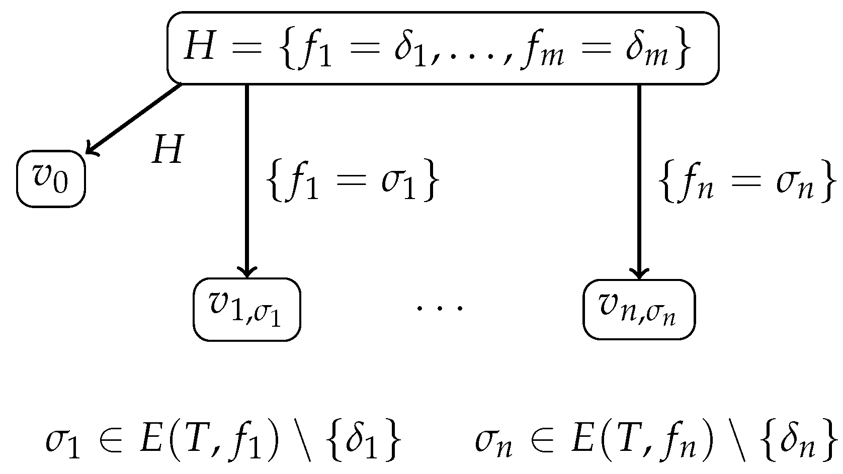
Let the root of
be labeled with a hypothesis
over
T that is admissible for
T; see
Figure 1, which depicts a prefix of the tree
. The root of
has a child
such that
. For each
and each
, the root of
has a child
such that
. The root of
has no other children.
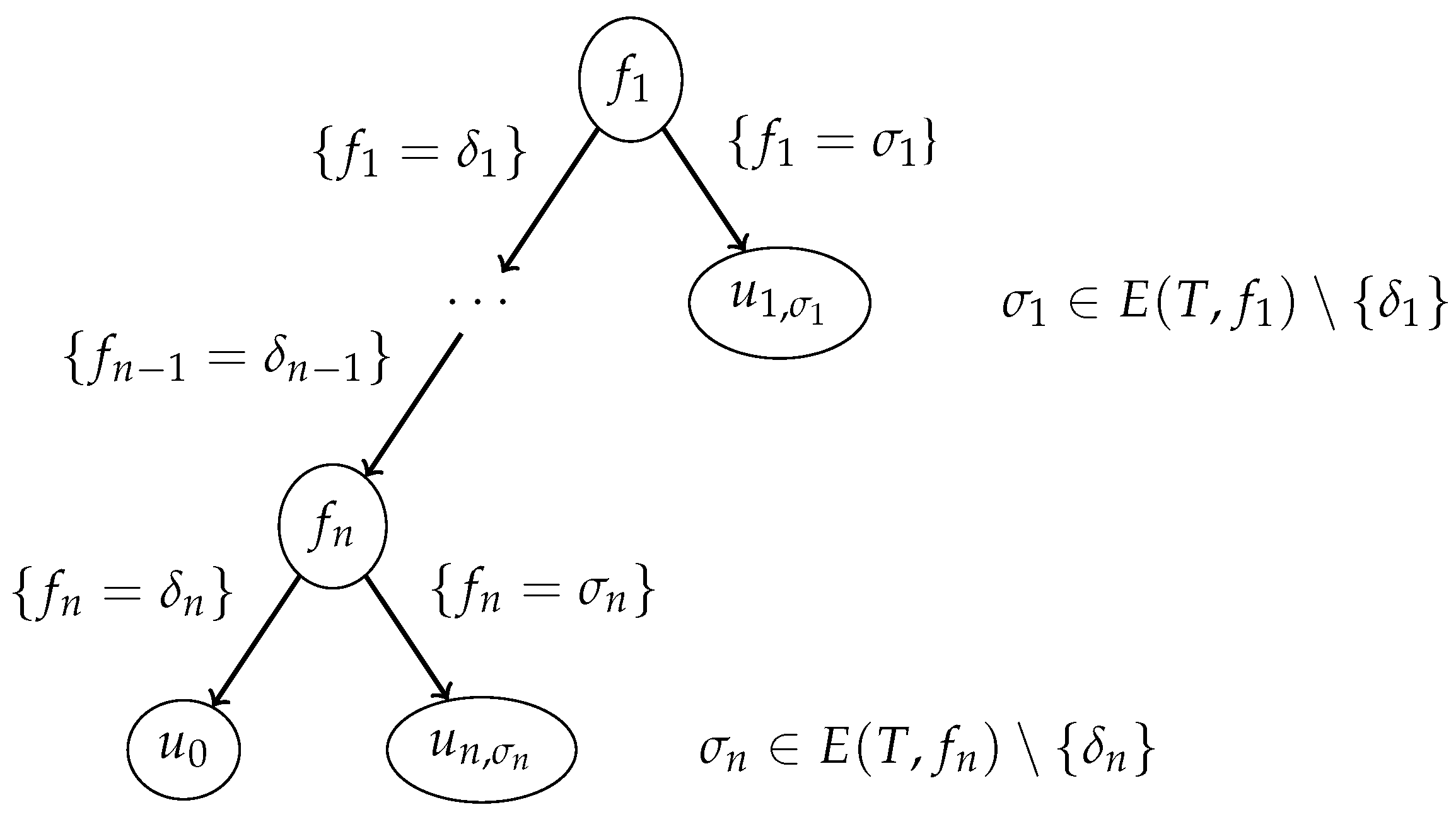
We transform the tree
into a decision tree
of the type 1 for the table
T; see
Figure 2, which depicts a prefix of the tree
. For the node
of the considered prefix,
. For each
and each
, the node of this prefix labeled with the attribute
has a child
such that
. It is clear that
is a subtable of
. By Lemma 9,
. It is also clear that
. Using the inductive hypothesis, we obtain that there is a decision tree
of the type 1 for the table
such that
.
We now transform the prefix of a decision tree
depicted in
Figure 2 into a decision tree
of the type 1 for the table
T. First, we transform the node
into a terminal node labeled with the number 0 if
is not a row of
T and labeled with the decision attached to
if this tuple is a row of
T. Next, for each
and each
, we replace the node
with the tree
. It is clear that the obtained tree
is a decision tree of the type 1 for the decision table
T and
.
We proved that, for any decision table T, ; hence, . □
10. Results of Experiments
We conducted experiments with eight decision tables from the UCI ML Repository [
20].
Table 1 contains information about each of these decision tables: its name, the number of rows, and the number of attributes. For each of the considered four cost functions, each of the considered five types of decision trees, and each of the considered eight decision tables, we find the minimum cost of a decision tree of the given type for the given table.
For , we randomly generate 100 Boolean functions with n variables. We represent each Boolean function f with n variables as a decision table with n columns labeled with variables considered as attributes and with rows that are all possible n-tuples of values of the variables. Each row is labeled with the decision that is the value of the function f on the corresponding n-tuple. We consider decision trees for the table as decision trees computing the function f.
For each of the considered four cost functions, each of the considered five types of decision trees, and each of the generated Boolean functions, using its decision table representation, we find the minimum cost of a decision tree of the given type computing this function.
The following remarks clarify some experimental results considered later.
From Proposition 10, it follows that for any decision table T.
Let
f be a Boolean function with
variables. Since each hypothesis over the decision table
is proper, the following equalities hold:
10.1. Depth
In this section, we consider some results obtained in Reference [
12]. Results of experiments with eight decision tables from Reference [
20] and the depth are represented in
Table 2. The first column contains the name of the considered decision table
T. The last five columns contain values
(minimum values for each decision table are in bold).
Decision trees with the minimum depth using attributes (type 1) are optimal for 5 decision tables, using hypotheses (type 2) are optimal for 4 tables, using attributes and hypotheses (type 3) are optimal for 8 tables, using proper hypotheses (type 4) are optimal for 3 tables, using attributes and proper hypotheses (type 5) are optimal for 7 tables.
For the decision table soybean-small, we must use attributes to construct an optimal decision tree. For this table, it is enough to use only attributes. For the decision tables breast-cancer and nursery, we must use both attributes and hypotheses to construct optimal decision trees. For these tables, it is enough to use attributes and proper hypotheses. For the decision table tic-tac-toe, we must use both attributes and hypotheses to construct optimal decision trees. For this table, it is not enough to use attributes and proper hypotheses.
Results of experiments with Boolean functions and the depth are represented in
Table 3. The first column contains the number of variables in the considered Boolean functions. The last five columns contain information about values
in the format
.
From the obtained results, it follows that, generally, the decision trees of the types 2 and 4 are better than the decision trees of the type 1, and the decision trees of the types 3 and 5 are better than the decision trees of the types 2 and 4.
10.2. Number of Realizable Nodes
In this section, we consider some results obtained in Reference [
13]. Results of experiments with eight decision tables from Reference [
20] and the number of realizable nodes are represented in
Table 4. The first column contains the name of the considered decision table
T. The last five columns contain values
(minimum values for each decision table are in bold).
Decision trees with the minimum number of realizable nodes using attributes (type 1) are optimal for 4 decision tables, using hypotheses (type 2) are optimal for 0 tables, using attributes and hypotheses (type 3) are optimal for 8 tables, using proper hypotheses (type 4) are optimal for 0 tables, and using attributes and proper hypotheses (type 5) are optimal for 8 tables.
Decision trees of the types 3 and 5 can be a bit better than the decision trees of the type 1. Decision trees of the types 2 and 4 are far from the optimal.
For the decision tables hayes-roth-data, soybean-small, tic-tac-toe, and zoo-data, we must use attributes to construct optimal decision trees. For these tables, it is enough to use only attributes. For the rest of the considered decision tables, we must use both attributes and hypotheses to construct optimal decision trees. For these tables, it is enough to use attributes and proper hypotheses.
Results of experiments with Boolean functions and the number of realizable nodes are represented in
Table 5. The first column contains the number of variables in the considered Boolean functions. The last five columns contain information about values
in the format
.
From the obtained results, it follows that, generally, the decision trees of the types 3 and 5 are slightly better than the decision trees of the type 1, and the decision trees of the types 2 and 4 are far from the optimal.
10.3. Number of Realizable Terminal Nodes
Results of experiments with eight decision tables from Reference [
20] and the number of realizable terminal nodes are represented in
Table 6. The first column contains the name of the considered decision table
T. The last five columns contain values
(minimum values for each decision table are in bold).
Decision trees of the types 1, 3, and 5 are optimal for each of the considered tables. Decision trees of the types 2 and 4 are far from the optimal.
Results of experiments with Boolean functions and the number of realizable terminal nodes are represented in
Table 7. The first column contains the number of variables in the considered Boolean functions. The last five columns contain information about values
in the format
.
From the obtained results, it follows that, generally, the decision trees of the types 1, 3, and 5 are optimal, and the decision trees of the types 2 and 4 are far from the optimal.
10.4. Number of Working Nodes
Results of experiments with eight decision tables from Reference [
20] and the number of working nodes are represented in
Table 8. The first column contains the name of the considered decision table
T. The last five columns contain values
(minimum values for each decision table are in bold).
Decision trees with the minimum number of working nodes using attributes (type 1) are optimal for 2 decision tables, using hypotheses (type 2) are optimal for 0 tables, using attributes and hypotheses (type 3) are optimal for 8 tables, using proper hypotheses (type 4) are optimal for 0 tables, using attributes and proper hypotheses (type 5) are optimal for 7 tables.
Decision trees of the types 3 and 5 can be a bit better than the decision trees of the type 1. Decision trees of the types 2 and 4 are far from the optimal.
For all decision tables with the exception of soybean-small and zoo-data, we must use both attributes and hypotheses to construct optimal decision trees. Moreover, for tic-tac-toe, it is not enough to use attributes and proper hypotheses. For soybean-small and zoo-data, it is enough to use only attributes to construct optimal decision trees.
Results of experiments with Boolean functions and the number of working nodes are represented in
Table 9. The first column contains the number of variables in the considered Boolean functions. The last five columns contain information about values
in the format
.
From the obtained results, it follows that, generally, the decision trees of the types 3 and 5 are better than the decision trees of the type 1, and the decision trees of the types 2 and 4 are far from the optimal.
We can now sum up the results of the experiments. Generally, the decision trees of the types 3 and 5 are slightly better than the decision trees of the type 1. Decision trees of the types 2 and 4 have, generally, too many nodes.
11. Conclusions
In this paper, we studied modified decision trees that use both queries based on one attribute each and queries based on hypotheses about values of all attributes. We designed dynamic programming algorithms for minimization of four cost functions for such decision trees and considered results of computer experiments. The main result of the paper is that the use of hypotheses can decrease the complexity of decision trees and make them more suitable for knowledge representation. In the future, we are planning to compare the length and coverage of decision rules derived from different types of decision trees constructed by the dynamic programming algorithms. Unfortunately, the considered algorithms cannot work together to optimize more than one cost function. In the future, we are also planning to consider two extensions of these algorithms: (i) sequential optimization relative to a number of cost functions and (ii) bi-criteria optimization that allows us to construct for some pairs of cost functions the corresponding Pareto front.


