
Modeling the Potential for Rural Tourism Development via GWR and MGWR in the Context of the Analysis of the Rural Lodging Supply in Extremadura, Spain

 ,
,  , ,
, ,
Abstract
:1. Introduction
- -
- Geostatistical models, specifically spatially weighted regressions (GWR) and multiscale geographically weighted regressions (MGWR), were used to determine the fit between the regressors (X1, X2..., Xn) and the predicted variable (Y). The former is understood to denote the types of tourism resources preferred by this type of demand. The latter, on the other hand, refers to the number of vacancies in rural tourism lodgings.
- -
- The use of this type of technique (GWR and MGWR) requires a series of preliminary investigations, in the course of which collinearity is eliminated by means of exploratory regressions.
- -
- The derivation of viable models enables the initial hypothesis to be corroborated or disproved.
2. Materials and Methods
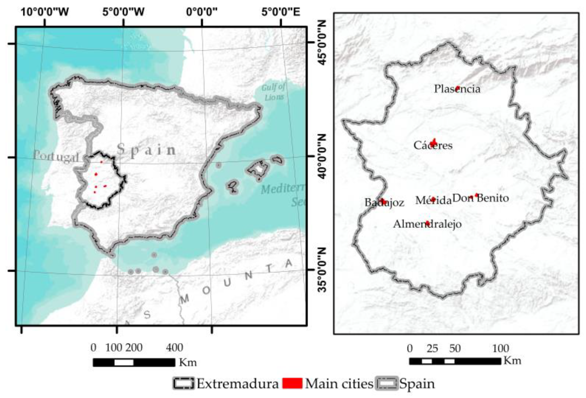
2.1. Study Area
2.2. Materials
2.3. Geostatistical Analysis
- -
- The model must be linear;
- -
- The data used should not depend on any external factor;
- -
- Explanatory variables should not be related to each other;
- -
- The explanatory variables must have a negligible measurement error;
- -
- The residuals must add up to 0; and
- -
- The residuals must have homogeneous variance and follow a normal distribution.
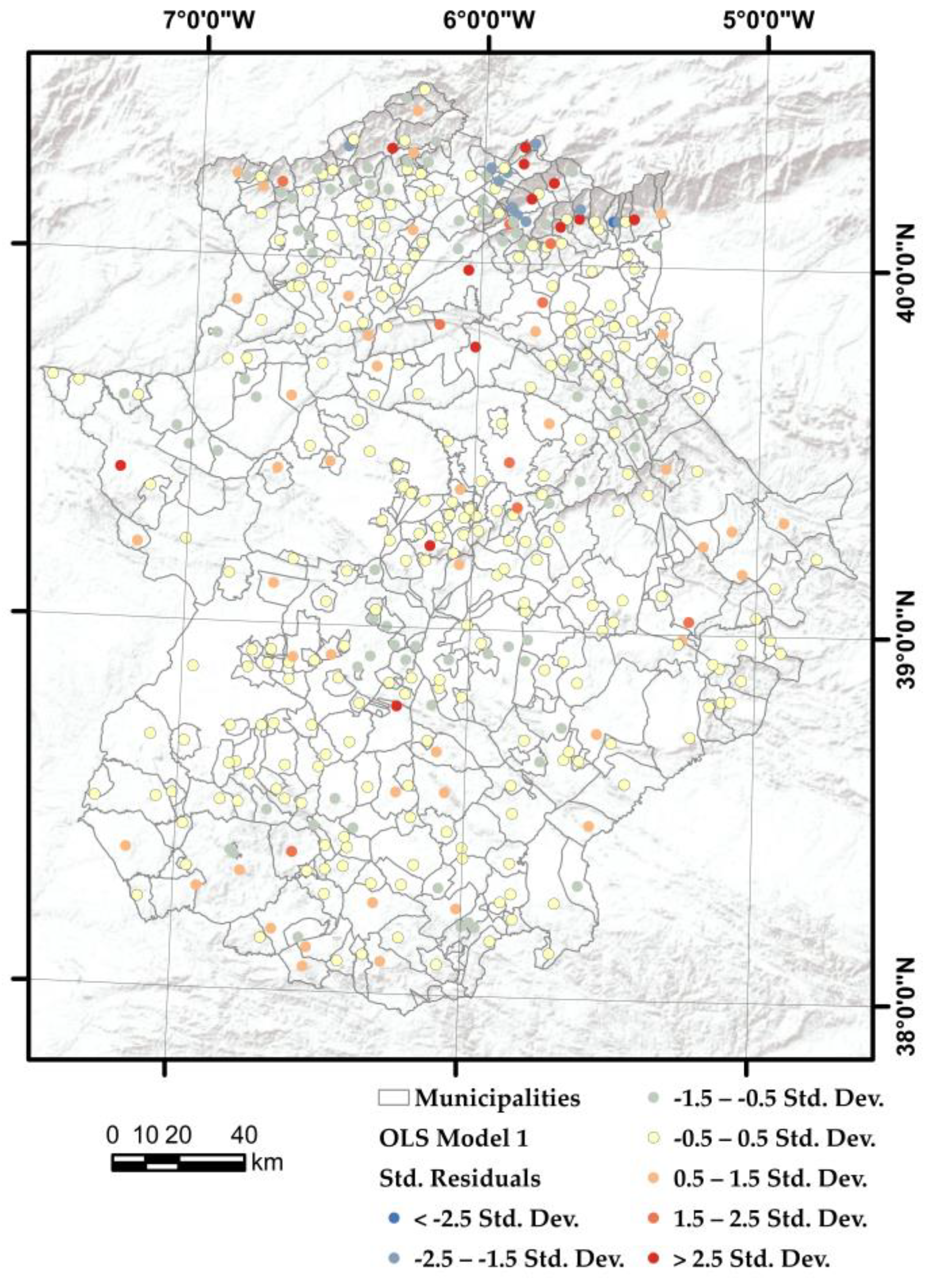
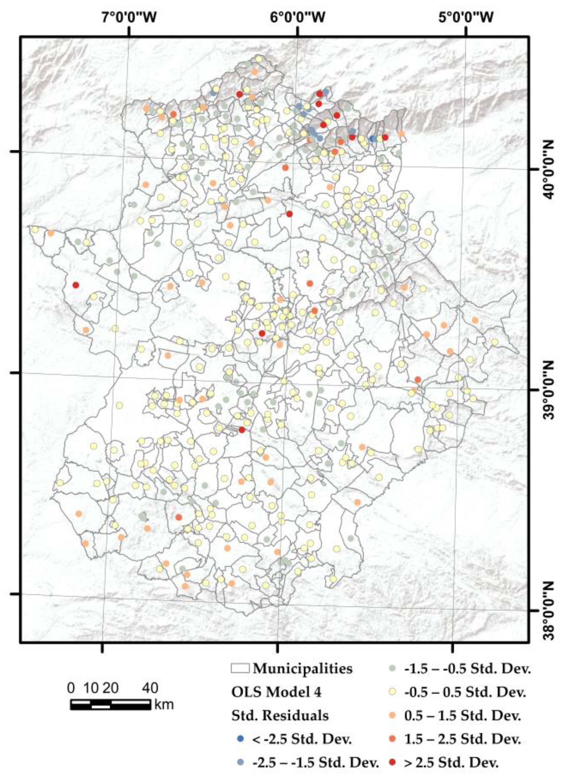
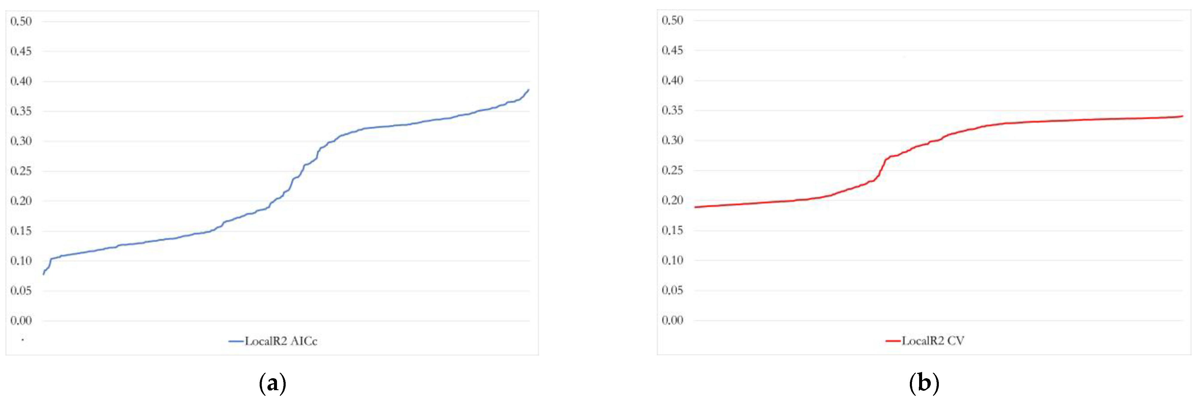
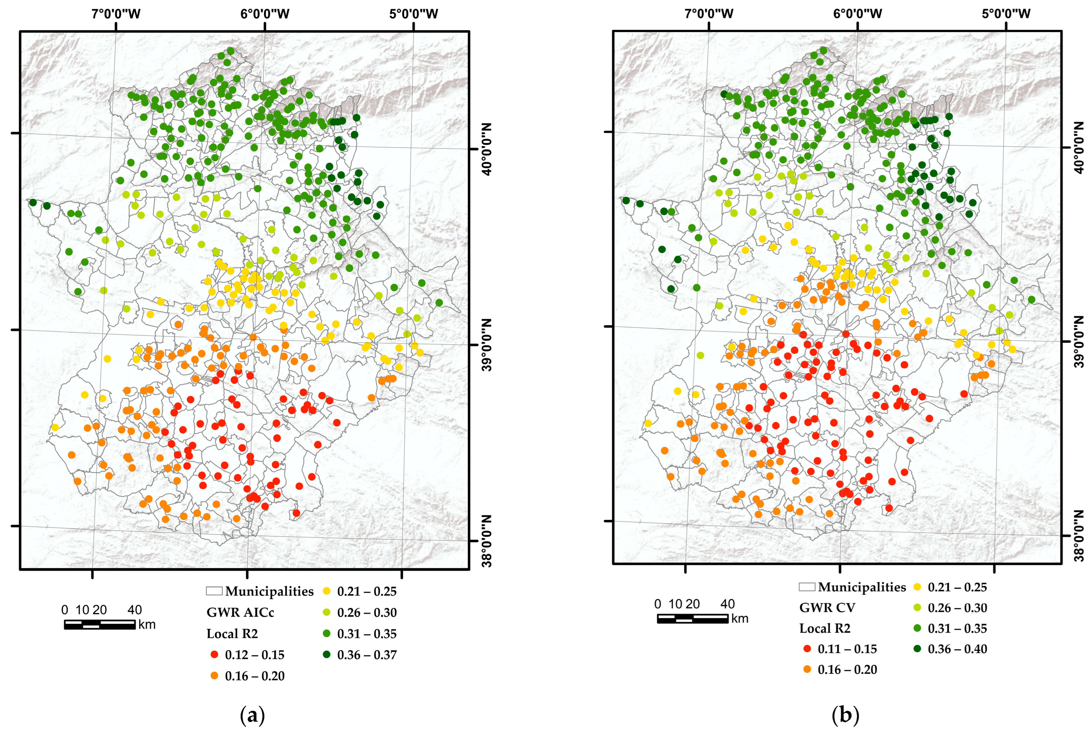
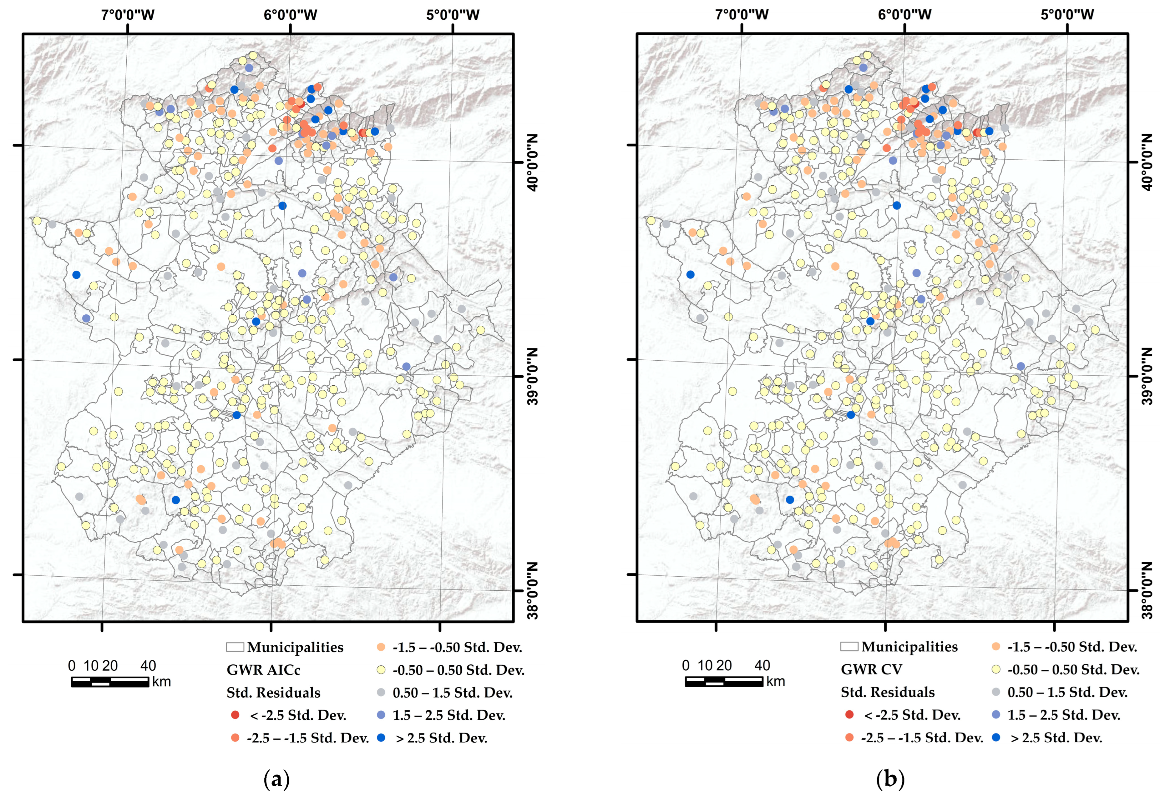
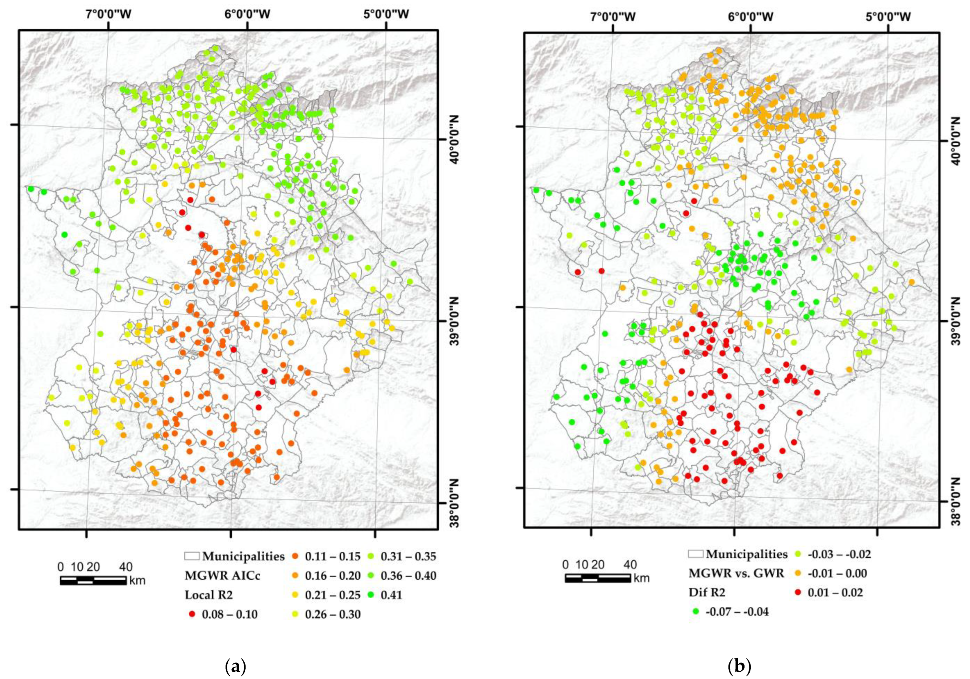
3. Results
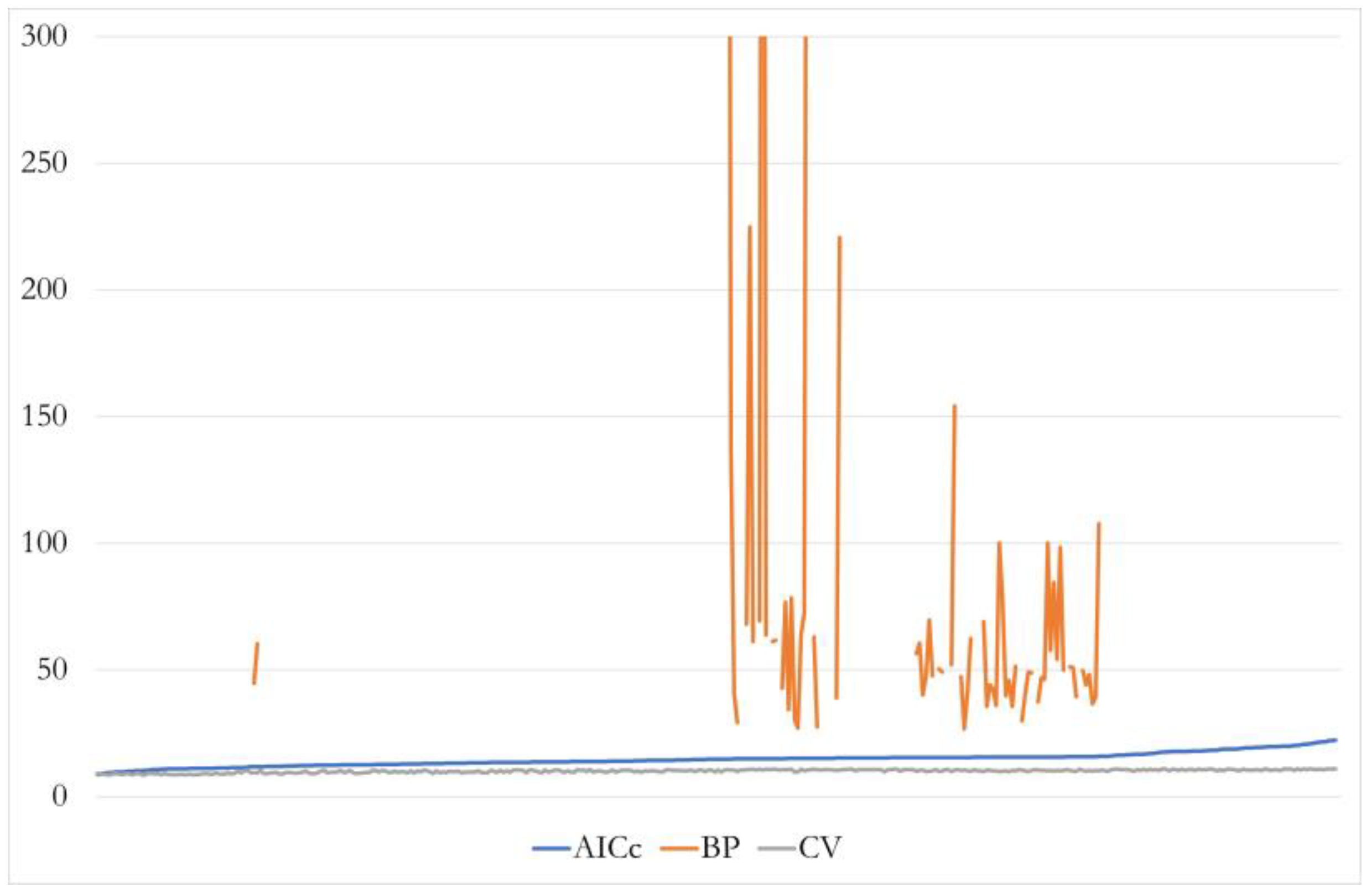
- -
- Kernel: adaptive; and
- -
- Bandwidth: AICc, CV, and BP following the neighbor criterion.
4. Discussion
5. Conclusions
Author Contributions
Funding
Data Availability Statement
Conflicts of Interest
References
- Rosalina, P.D.; Dupre, K.; Wang, Y. Rural tourism: A systematic literature review on definitions and challenges. J. Hosp. Tour. Manag. 2021, 47, 134–149. [Google Scholar] [CrossRef]
- Gilbert, D. Rural tourism and marketing: Synthesis and new ways of working. Tour. Manag. 1989, 10, 39–50. [Google Scholar] [CrossRef]
- Hernández Maestro, R.M.; Muñoz Gallego, P.A.; Santos Requejo, L. The moderating role of familiarity in rural tourism in Spain. Tour. Manag. 2007, 28, 951–964. [Google Scholar] [CrossRef]
- Lane, B.; Kastenholz, E. Rural tourism: The evolution of practice and research approaches—towards a new generation concept? J. Sustain. Tour. 2015, 23, 1133–1156. [Google Scholar] [CrossRef]
- Tirado-Ballesteros, J.G. La funcionalidad turística de los espacios rurales: Conceptualización y factores de desarrollo. Cuad. Geográficos De La Univ. De Granada 2017, 56, 312–332. Available online: https://revistaseug.ugr.es/index.php/cuadgeo/article/view/5342 (accessed on 19 November 2022).
- Lane, B. What is rural tourism? J. Sustain. Tour. 1994, 2, 7–21. [Google Scholar] [CrossRef]
- Quaranta, G.; Citro, E.; Salvia, R. Economic and Social Sustainable Synergies to Promote Innovations in Rural Tourism and Local Development. Sustainability 2016, 8, 668. [Google Scholar] [CrossRef]
- Fang, W.T. Rural Tourism. In Tourism in Emerging Economies; Springer: Singapore, 2020. [Google Scholar] [CrossRef]
- Lulcheva, I.; Aleksandrov, K. Research on the supply and consumer demand for rural tourism in Eastern Rhodopes. Sci. Pap. Ser. Manag. Econ. Eng. Agric. Rural. Dev. 2017, 17, 179–185. Available online: http://www.managementjournal.usamv.ro/pdf/vol.17_4/volume_17_4_2017.pdf (accessed on 12 January 2023).
- Trukhachev, A. Methodology for Evaluating the Rural Tourism Potentials: A Tool to Ensure Sustainable Development of Rural Settlements. Sustainability 2015, 7, 3052–3070. [Google Scholar] [CrossRef]
- Xie, Y.; Meng, X.; Cenci, J.; Zhang, J. Spatial Pattern and Formation Mechanism of Rural Tourism Resources in China: Evidence from 1470 National Leisure Villages. ISPRS Int. J. Geo-Inf. 2022, 11, 455. [Google Scholar] [CrossRef]
- Qiao, H.H.; Wang, C.-H.; Chen, M.-H.; Su, C.-H.J.; Tsai, C.-H.K.; Liu, J. Hedonic price analysis for high-end rural homestay room rates. J. Hosp. Tour. Manag. 2021, 49, 1–11. [Google Scholar] [CrossRef]
- Sánchez Martín, J.M.; Sánchez Rivero, M.; Rengifo Gallego, J. The evaluation of the potential for the development of rural tourism. Methodological application on the province of Cáceres. Geofocus Int. J. Geogr. Inf. Sci. Technol. 2013, 13, 99–130. Available online: http://www.geofocus.org/index.php/geofocus/article/view/263/111 (accessed on 18 January 2023).
- Sánchez Rivero, M.; Sánchez Martín, J.M. New Research Techniques Applied to Tourism: Spatial Statistics. In Modelos de Gestión e Innovación en Turismo; Figuerola Palomo, M., Martín Duque, C., Eds.; Civitas Thomson Reuters: Madrid, Spain, 2019; pp. 109–132. [Google Scholar] [CrossRef]
- Tobler, W. A computer movie simulating urban growth in the Detroit region. Econ. Geogr. 1970, 46, 234–240. [Google Scholar] [CrossRef]
- Sánchez Martín, J.; Pérez Martín, M.; Jurado Rivas, J.; Granados Claver, M. Detection of optimal areas for the implementation of rural accommodation in Extremadura. A GIS Appl. Lurralde Res. Space 1999, 22, 367–384. Available online: http://www.ingeba.org/lurralde/lurranet/lur22/sanch22/sanch22.htm (accessed on 15 November 2022).
- Cressie, N. Geostatistics. Am. Stat. 1989, 43, 197–202. Available online: https://www.jstor.org/stable/2685361 (accessed on 19 December 2022).
- Diggle, P.J.; Tawn, J.A.; Moyeed, R.A. Model-based geostatistics. J. R. Stat. Soc. Ser. C (Appl. Stat.) 1998, 47, 299–350. [Google Scholar] [CrossRef]
- Webster, R.; Oliver, M.A. Geostatistics for Environmental Scientists; John Wiley & Sons: Hoboken, NJ, USA, 2007. [Google Scholar] [CrossRef]
- Chiles, J.P.; Delfiner, P. Geostatistics: Modeling Spatial Uncertainty, 2nd ed.; John Wiley & Sons: Hoboken, NJ, USA, 2009. [Google Scholar]
- Matheron, G. Principles of Geostatistics. Econ. Geol. 1963, 58, 1246–1260. [Google Scholar] [CrossRef]
- Matheron, G. The Theory of Regionalized Variables and its Applications; Ecole Nationale Supérieure des Mines de Paris: Paris, France, 1971. [Google Scholar]
- Zheng, F.; Hou, Y.; Yang, K. Spatial Statistics Methods and Relative Software Application in Tourism Studies. Stat. Appl. 2017, 6, 380–385. [Google Scholar]
- Pira, M.L.; Gemma, A.; Gatta, V.; Carrese, S.; Marcucci, E. Walking and Sustainable Tourism: “Streetsadvisor.” A Stated Preference GIS-Based Methodology for Estimating Tourist Walking Satisfaction in Rome. Transp. Sustain. 2021, 13, 45–58. [Google Scholar] [CrossRef]
- Adabi, G.; Hajiha, A.; Hosseinzadhe, F. Designing a tourism industry model in Iran with the approach of the spatial correlation structure. J. Ind. Eng. Manag. Stud. 2022, 8, 261–276. [Google Scholar] [CrossRef]
- Alonzo Hernández, K.; Chávez Gonzáles, O.; López Arellano, A.; Carranza Bello, J. Geostatistics applied to the analysis of spatial variability. Innova Ing. J. 2018, 1, 60–66. Available online: https://www.innovaingenieria.uagro.mx/innova/index.php/innova/article/view/17/21 (accessed on 16 January 2023).
- Zapata Salcedo, J.; Gómez Ramos, A. Ethos and praxis of the quantitative revolution in geography. J. Int. Relat. Strategy Secur. 2008, 3, 189–202. [Google Scholar] [CrossRef]
- Smith, S. Room for Rooms: A Procedure for the Estimation of Potential Expansion of Tourits Accommodations. J. Travel Res. 1977, 15, 26–29. [Google Scholar] [CrossRef]
- Liu, Z.; Lan, J.; Chien, F.; Sadiq, M.; Nawaz, M.A. Role of tourism development in environmental degradation: A step towards emission reduction. J. Environ. Manag. 2022, 303, 114078. [Google Scholar] [CrossRef]
- Wang, X.; Sun, J.; Wen, H. Tourism seasonality, online user rating and hotel price: A quantitative approachbased on the hedonic price model. Int. J. Hosp. Manag. 2019, 79, 140–147. [Google Scholar] [CrossRef]
- Yang, Y.; Luo, H.; Law, R. Theoretical, empirical, and operational models in hotel location research. Int. J. Hosp. Manag. 2014, 36, 209–220. [Google Scholar] [CrossRef]
- Yong-Feng, Z.; Wahap, H.; Chen, H. Spatial heterogeneity and optimization strategies of tourism attractions in Xinjiangbased on the GWR mode. J. Nat. Sci. Hunan Norm. Univ. 2017, 40, 1–8. [Google Scholar]
- Shabrina, Z.; Buyuklieva, B.; Ming, M.N.K. Airbnb, hotels, and saturation of the food industry: A multi-scale GWR approach. arXiv 2019, arXiv:1905.12543v2. [Google Scholar]
- Liu, J.; Yue, M.; Liu, Y.; Wen, D.; Tong, Y. The Impact of Tourism on Ecosystem Services Value: A Spatio-Temporal Analysis Based on BRT and GWR Modeling. Sustainability 2022, 14, 2587. [Google Scholar] [CrossRef]
- Fotheringham, A.S.; Yang, W.; Kang, W. Multiscale geographically weighted regression (MGWR). Ann. Am. Assoc. Geogr. 2017, 107, 1247–1265. [Google Scholar] [CrossRef]
- Hernández, J.M.; Suárez-Vega, R.; Santana-Jiménez, Y. The inter-relationship between rural and mass tourism: The case of Catalonia, Spain. Tour. Manag. 2016, 54, 43–57. [Google Scholar] [CrossRef]
- Shabrina, Z.; Buyuklieva, B.; NG, M. Short-term rental platform in the urban tourism context: A geographically weighted regression (GWR) and a multiscale GWR (MGWR) approaches. Geogr. Anal. 2021, 53, 686–707. [Google Scholar] [CrossRef]
- Watson, P.; Deller, S. Tourism and economic resilience. Tour. Econ. 2022, 28, 1193–1215. [Google Scholar] [CrossRef]
- Fonseca, N.; Sáncher Rivero, M. Granger Causality between Tourism and Income: A Meta-regression Analysis. J. Travel Res. 2019, 59, 642–660. [Google Scholar] [CrossRef]
- Rodríguez Rangel, M.; Sánchez Rivero, M.; Ramajo Hernández, J. Spatial Intensity in Tourism Accommodation: Modelling Differences in Trends for Several Types through Poisson Models. ISPRS Int. J. Geo-Inf. 2020, 9, 473. [Google Scholar] [CrossRef]
- Sánchez Rivero, M.; Rodríguez Rangel, M.; Fernández Torres, Y. The Identification of Factors Determining the Probability of Practicing Inland Water Tourism Through Logistic Regression Models: The Case of Extremadura, Spain. Water 2020, 12, 1664. [Google Scholar] [CrossRef]
- Sánchez Martín, J.; Sánchez Rivero, M.; Rengifo Gallego, J. Patterns of tourism supply distribution using geostatistical techniques in Extremadura (2004–2014). Boletín De La Asoc. De Geógrafos Españoles 2018, 76, 276–302. [Google Scholar] [CrossRef]
- Sánchez Martín, J. El Sistema de Información Geográfica como herramienta de análisis turísitico. Una aplicación para la localización idónea de alojamientos rurales en la provincia de Cáceres mediante análisis multicriterio. Estud. Turísticos 2009, 182, 71–94. [Google Scholar]
- Sánchez Martín, J.; Sánchez Rivero, M.; Rengifo Gallego, J. Analysis of the balance between tourist potential and supply of rural tourism accommodation using spatial statistical techniques. Appl. Prov. Cáceres (Spain). Cuad. De Tur. 2017, 39, 699–702. Available online: http://revistas.um.es/turismo/article/download/290701/212541 (accessed on 15 September 2022).
- Sánchez-Martín, J.-M.; Rengifo-Gallego, J.-I.; Martín-Delgado, L.-M.; Hernández Carretero, A.-M. Methodological System to Determine the Development Potential of Rural Tourism in Extremadura, Spain. Systems 2022, 10, 153. [Google Scholar] [CrossRef]
- Campesino Fernández, A.-J. (Ed.) Territorial Characterization of the Extremadura Border. In Turismo de Frontera (I); RIET: Santiago de Compostela, Spain, 2013. [Google Scholar]
- National Statistics Institute (INE). Cifras Oficiales de Población de Los Municipios Españoles en Aplicación de la Ley de Bases del Régimen Local (Art. 17). 2022. Available online: https://ine.es/dynt3/inebase/es/index.htm?padre=525 (accessed on 20 February 2023).
- Sánchez Martín, J. Municipal tourism typology of Extremadura based on principal component factor analysis. Lurralde Res. Space 1998, 21, 95–119. Available online: http://www.ingeba.org/lurralde/lurranet/lur21/21sanche/21sanch.htm (accessed on 19 October 2022).
- Sánchez Martín, J.; Rengifo Gallego, J. Evolution of the tourism sector in 21st century Extremadura: Boom, crisis and recovery. Lurralde: Res. Space 2019, 42, 19–50. Available online: http://www.ingeba.org/lurralde/lurranet/lur42/42sanchez.pdf (accessed on 19 October 2022). [CrossRef]
- Gil Álvarez, L.; Martín Delgado, L.; Sánchez Martín, J. Heritage resources in rural Extremadura: Design, planning and management of tourist-cultural itineraries. Lurralde Res. Space 2021, 44, 657–690. Available online: http://www.ingeba.org/lurralde/lurranet/lur44/Lurralde-44-2021_Luz.pdf (accessed on 19 October 2022). [CrossRef]
- Sánchez Martín, J.M.; Rengifo Gallego, J.I.; Sánchez Rivero, M. Protected areas as a centre of attraction for visitors to the surroundins: Extremad (Spain). Land 2020, 9, 47. [Google Scholar] [CrossRef]
- Sánchez Martín, J.M.; Rengifo Gallego, J.I.; Jiménez Barrado, V. Rental housing (Airbnb) and traditional tourist accommodation: New competitive scenario in the Extremadura tourism market. Estud. Geográficos 2019, 80, 1–14. [Google Scholar] [CrossRef]
- Official State Gazette. Law 2/2011, of January 31, on the Development and Modernization of Tourism in Extremadura. Available online: https://www.boe.es/buscar/pdf/2011/BOE-A-2011-3179-consolidado.pdf (accessed on 15 October 2022).
- National Institute of Statistics (INE). Rural Tourism Accommodation Occupancy Survey (EOTR). 2022. Available online: https://www.ine.es/dyngs/INEbase/es/operacion.htm?c=Estadistica_C&cid=1254736176963&menu=resultados&idp=1254735576863#tabs-1254736195429 (accessed on 25 February 2023).
- National Institute of Statistics (INE). Available online: https://ine.es/ (accessed on 25 February 2023).
- Regional Government of Extremadura. Tourism Activities Register. Available online: https://www.juntaex.es/temas/turismo-y-cultura/actividades-turisticas (accessed on 25 February 2023).
- Regional Government of Extremadura. Tourism Observatory of Extremadura. Studies of 2017. Available online: https://www.turismoextremadura.com/.content/observatorio/2017/EstudiosYMemoriasAnuales/Anuario_oferta-demanda2017.pdf (accessed on 25 February 2023).
- National Geographic Institute (IGN). National Topographic Base 1:100,000 (BTN100). Available online: http://www.ign.es/web/resources/docs/IGNCnig/CBG%20-%20BTN100.pdf (accessed on 15 September 2022).
- IDEEX. Spatial Data Infrastructure of Extremadura. Available online: http://www.ideextremadura.com/Geoportal/files/articulos/Mapa_paisaje_Extremadura.pdf (accessed on 15 September 2022).
- Etxeberría, J. Multiple Regression; La Muralla: Madrid, Spain, 2007. [Google Scholar]
- Fotheringhan, A.; Charlton, M.; Brunsdon, C. Geographically weighted regression: A natural evolution of the expansion method for spatial data analysis. Environ. Plan. A Econ. Space 1998, 30, 1905–1927. [Google Scholar] [CrossRef]
- Lu, B.; Charlton, M.; Harris, P.; Fotheringham, A.S. Geographically weighted regression with a non-Euclidean distance metric: A case study using hedonic house price data. Int. J. Geogr. Inf. Sci. 2014, 28, 660–681. [Google Scholar] [CrossRef]
- Gao, C.; Feng, Y.; Tong, X.; Lei, Z.; Chen, S.; Zhai, S. Modeling urban growth using spatially heterogeneous cellular automata models: Comparison of spatial lag, spatial error and GWR. Comput. Environ. Urban Syst. 2020, 81, 101459. [Google Scholar] [CrossRef]
- Lu, B.; Yang, W.; Ge, Y.; Harris, P. Improvements to the calibration of a geographically weighted regression with parameter-specific distance metrics and bandwidths. Comput. Environ. Urban Syst. 2018, 71, 41–57. [Google Scholar] [CrossRef]
- Bouza Herrera, C. Regression Models and Their Applications. Available online: https://www.researchgate.net/publication/323227561_MODELOS_DE_REGRESION_Y_SUS_APLICACIONES#read (accessed on 17 October 2021).
- Santos, C.; Cabral, J. An Analysis of Visitors’ Expenditures in a Tourist Destination: OLS, Quantile Regression and Instrumental Variable Estimators. Tour. Econ. 2012, 18, 555–576. [Google Scholar] [CrossRef]
- Brida, J.; Scuderi, R. Determinants of tourist expenditure: A review of microeconometric models. Tour. Manag. Perspect. 2013, 6, 28–40. [Google Scholar] [CrossRef]
- Meloun, M.; Jiří Militký, J. Detection of single influential points in OLS regression model building. Anal. Chim. Acta 2001, 439, 169–191. [Google Scholar] [CrossRef]
- Wilcox, R. Robust regression: Testing global hypotheses about the slopes when there is multicollinearity or heteroscedasticity. Br. J. Math. Stat. Psychol. 2018, 72, 355–369. [Google Scholar] [CrossRef]
- Wilcox, R. Multicolinearity and ridge regression: Results on type I errors, power and heteroscedasticity. J. Appl. Stat. 2019, 46, 946–957. [Google Scholar] [CrossRef]
- Sánchez Martín, J.M. The linear correlation matrix in Climatology. Interpretative risks: Their reduction or elimination. Estud. Geográficos 1995, 56, 411–434. [Google Scholar] [CrossRef]
- Berry, W. Understanding Regression Assumptions; SAGE: Newbury Park, CA, USA, 1993. [Google Scholar]
- Getis, A.; Ord, K. The Analysis of Spatial Association by Use of Distance Statistics. Geogr. Anal. 1992, 24, 189–206. [Google Scholar] [CrossRef]
- Anselin, L. Local Indicators of Spatial Association—LISA. Geogr. Anal. 1995, 27, 93–115. [Google Scholar] [CrossRef]
- Tu, J.; Xia, Z.-G. Examining spatially varying relationships between land use and water quality using geographically weighted regression I: Model design and evaluation. Sci. Total Environ. 2008, 407, 358–378. [Google Scholar] [CrossRef] [PubMed]
- Sánchez Martín, J.M.; Rengifo Gallego, J.I.; Blas Morato, R. Hot Spot Analysis versus Cluster and Outlier Analysis: An Enquiry into the Grouping of Rural Accommodation in Extremadura (Spain). ISPRS Int. J. Geo-Inf. 2019, 8, 176. [Google Scholar] [CrossRef]
- De Toro, P.; Nocca, F.; Renna, A.; Sepe, L. Real Estate Market Dynamics in the City of Naples: An Integration of a Multi-Criteria Decision Analysis and Geographical Information System. Sustainability 2020, 12, 1211. [Google Scholar] [CrossRef]
- ESRI. Documentation. Available online: https://doc.arcgis.com/es/insights/analyze/regression-analysis.htm (accessed on 19 September 2022).
- ESRI (n.d.). Network Analyst. Available online: https://desktop.arcgis.com/es/arcmap/latest/extensions/network-analyst/service-area.htm (accessed on 19 September 2022).
- Brunsdon, C.; Fotheringham, A.S.; Charlton, M. Spatial Nonstationarity and Autoregressive Models. Environ. Plan. A Econ. Space 1998, 30, 957–973. [Google Scholar] [CrossRef]
- Wu, B.; Yan, J.; Lin, H. A cost-effective algorithm for calibrating multiscale geographically weighted regression models. Int. J. Geogr. Inf. Sci. 2021, 36, 898–917. [Google Scholar] [CrossRef]
- Li, Z.; Oshan, T.; Fotheringham, S.; Kang, W.; Wolf, L.; Sachdeva, M.; Bardin, S. MGWR 2.2. User Manual. Available online: https://sgsup.asu.edu/sites/default/files/SparcFiles/mgwr_2.2_manual_final.pdf (accessed on 14 November 2022).
- Morrissey, M.; Ruxton, G. Multiple Regression Is Not Multiple Regressions: The Meaning of Multiple Regression and the Non-Problem of Collinearity. Philos. Theory Pract. Biol. 2018, 10, 1–24. [Google Scholar] [CrossRef]
- Keith, T. Multiple Regression and Beyond. An Introduction to Multiple Regression and Structural Equation Modeling; Routledge: New York, NY, USA, 2019. [Google Scholar] [CrossRef]
- Allen, M. (Ed.) The Problem of Multicollienarity. In The Problem of Multicollinearity. In Understanding Regression Analysis; Springer: Boston, MA, USA, 1997; pp. 176–180. [Google Scholar] [CrossRef]
- Chen, Y.; Zhu, M.; Zhou, Q.; Qiao, Y. Research on Spatiotemporal Differentiation and Influence Mechanism of Urban Resilience in China Based on MGWR Model. Int. J. Environ. Res. Public Health 2021, 18, 1056. [Google Scholar] [CrossRef] [PubMed]
- Oshan, T.; Li, Z.; Kang, W.; Wolf, L.; Fotheringham, A. mgwr: A Python Implementation of Multiscale Geographically Weighted Regression for Investigating Process Spatial Heterogeneity and Scale. ISPRS Int. J. Geo-Inf. 2019, 8, 269. [Google Scholar] [CrossRef]
- Liu, N.; Strobl, J. Impact of neighborhood features on housing resale prices in Zhuhai (China) based on an (M)GWR model. Big Earth Data 2023, 7, 156–179. [Google Scholar] [CrossRef]
- Comber, A.; Harris, P.; Brunsdon, C. A Route Map for Successful Applications of Geographically Weighted Regression. Geogr. Anal. 2022, 55, 155–178. [Google Scholar] [CrossRef]
- MGWR. SPARC—Multiscale Geographically Weighted Regression | School of Geographical Sciences & Urban Planning (asu.edu). Available online: https://sgsup.asu.edu/sparc/multiscale-gwr (accessed on 15 November 2022).
- Cànoves, G.; Villarino, M.; Herrera, L. Public policies, rural tourism and sustainability: Difficult balance. Boletín De La A.G.E. 2006, 41, 199–217. Available online: https://www.bage.age-geografia.es/ojs/index.php/bage/article/download/1997/1910/1978 (accessed on 15 November 2022).
- Song, H.; Xie, K.; Park, J.; Chen, W. Impact of accommodation sharing on tourist attractions. Ann. Tour. Res. 2020, 80, 102820. [Google Scholar] [CrossRef]
- Biswas, T.; Rai, A. Analysis of spatial patterns and driving factors of domestic medical tourism demand in North East India. GeoJournal 2022. [Google Scholar] [CrossRef]
- Arbel, A.; Pizam, A. Some Determinants of Urban Hotel Location: The Tourists’ Inclinations. J. Travel Res. 1977, 15, 18–22. [Google Scholar] [CrossRef]
- Sánchez-Martín, J.-M.; Blas-Morato, R.; Rengifo-Gallego, J.-I. The Dehesas of Extremadura, Spain: A Potential for Socio-Economic Development Based on Agritourism Activities. Forests 2019, 10, 620. [Google Scholar] [CrossRef]
- Junta de Extremadura. Estrategia de Turismo Sostenible de Extremadura 2030, II Plan Turístico de Extremadura 2021–2023. Available online: https://www.ugtextremadura.org/sites/www.ugtextremadura.org/files/estrategia_2030_ii_plan_turistico_extremadura_2021-2023.pdf (accessed on 18 April 2023).
- Gutiérrez, A.; Domènech, A. Understanding the spatiality of short-term rentals in Spain: Airbnb and the intensification of the commodification of housing. Geogr. Tidsskr.-Dan. J. Geogr. 2020, 120, 98–113. [Google Scholar] [CrossRef]
- Sánchez-Martín, J.-M.; Gurría-Gascón, J.-L.; Rengifo-Gallego, J.-I. The Distribution of Rural Accommodation in Extremadura, Spain-between the Randomness and the Suitability Achieved by Means of Regression Models (OLS vs. GWR). Sustainability 2020, 12, 4737. [Google Scholar] [CrossRef]
- Sánchez-Martín, J.-M.; Gurría-Gascón, J.-L.; García-Berzosa, M.-J. The Cultural Heritage and the Shaping of Tourist Itineraries in Rural Areas: The Case of Historical Ensembles of Extremadura, Spain. ISPRS Int. J. Geo-Inf. 2020, 9, 200. [Google Scholar] [CrossRef]
- Martín-Delgado, L.-M.; Jiménez-Barrado, V.; Sánchez-Martín, J.-M. Sustainable Hunting as a Tourism Product in Dehesa Areas in Extremadura (Spain). Sustainability 2022, 14, 10288. [Google Scholar] [CrossRef]


| Travelers | Overnight Stay- Ciones | EstanciaHalf | Grade of Occupation | Degree of Occupation F/Week | Establishment Mientos | Places | Employment | Overnight Stays /Plaza | |
|---|---|---|---|---|---|---|---|---|---|
| 2001 | 30,192 | 66,548 | 2.09 | 23.31 | NA | 104 | 939 | 172 | 70.9 |
| 2005 | 65,815 | 146,220 | 2.13 | 18.88 | NA | 228 | 2668 | 397 | 54.8 |
| 2010 | 107,526 | 251,518 | 2.29 | 14.14 | 22.17 | 461 | 5496 | 719 | 45.8 |
| 2015 | 161,011 | 349,386 | 2.12 | 19.87 | 28.79 | 538 | 6515 | 795 | 53.6 |
| 2019 | 226,723 | 499,749 | 2.20 | 17.89 | 34.64 | 632 | 7609 | 1001 | 65,7 |
| 2020 | 110,065 | 271,571 | 2.47 | 13.42 | 22.17 | 466 | 5598 | 737 | 48,5 |
| 2021 | 184,975 | 433,665 | 2.34 | 15.51 | 28.04 | 664 | 7584 | 954 | 57.2 |
| 2022 * | 238,897 | 533,431 | 2.19 | 17.26 | 31.70 | 725 | 8355 | 1153 | 66.2 |
| Internal Variables Considered (Type, Subtype and Code) | |||||
|---|---|---|---|---|---|
| Type | Subtype | Code | Type | Subtype | Code |
| Relief | Mountains and their foothills | VI1 | Summer thermal comfort | Average maximum temperature from June to September | VI22 |
| Saws | VI2 | Others | Big game hunting + 1000 hectares. | VI23 | |
| Piedemontes | VI3 | Long-distance trails | VI24 | ||
| Lakesides and valleys | VI4 | Short-distance trails | VI25 | ||
| Sedimentary basins/plains and peneplains | VI5 | Local trails | VI26 | ||
| Hydrography | Rivers (up to 2 km) | VI6 | Optimal visiting period (demand preferences) | VI27 | |
| Reservoirs | VI7 | Singularity (pairwise) | VI28 | ||
| Bathing areas | VI8 | Attractiveness according to demand (questionnaire) | VI29 | ||
| Waterfalls | VI9 | Proximity to main tourist attractions (EOH) | VI30 | ||
| Protected natural areas | National Park | VI10 | Proximity to tourist area (EOTR) | VI31 | |
| Park or Nature Reserve | VI11 | Population size | VI32 | ||
| Natural Monument | VI12 | Vegetation species | VI33 | ||
| ZEPA | VI13 | Geosites | VI34 | ||
| ZEC | VI14 | Viewpoints | VI35 | ||
| Cultural/historical-artistic heritage | Distance to World Heritage City (time) | VI15 | Observation points | VI36 | |
| Historic-artistic site | VI16 | Greenways | VI37 | ||
| Assets of Cultural Interest (Monuments) | VI17 | ||||
| Museums and collections | VI18 | ||||
| Livestock trails at 2 km | VI19 | ||||
| Castles | VI20 | ||||
| Archaeological sites | VI21 | ||||
| Considered external variables (type, subtype, and code) | |||||
| Type | Subtype | Code | Type | Subtype | Code |
| Hotel accommodation Accommodation (beds) | Hotel | VE1 | Others | Activity companies (no.) | VE13 |
| Hotel–Apartment | VE2 | Tourist guides (no.) | VE14 | ||
| Hostel | VE3 | Tourist offices | VE15 | ||
| Pension | VE4 | Interpretation centers | VE16 | ||
| Non-hotel accommodation (vacancies) | Tourist apartment | VE5 | Wharfs | VE17 | |
| Camping | VE6 | Accessibility | Highway | VE18 | |
| Rural lodging (vacancies) | Rural hotel | VE7 | National highway | VE19 | |
| Rural house | VE8 | Autonomous highway | VE20 | ||
| Rural apt. | VE9 | Main bus stations | VE21 | ||
| Restoration | Three- and four-fork restaurants (seats) | VE10 | Train stations | VE22 | |
| One- and two-fork restaurants (seats) | VE11 | Airport | VE23 | ||
| Café-bar (no.) | VE12 | ||||
| Search Criteria | Cut | Testing | No. of Accepted | % Accepted |
|---|---|---|---|---|
| R2 adjusted minimum | >0.3 | 261,800 | 44,362 | 16.94 |
| Maximum coefficient p value | <0.05 | 261,800 | 1269 | 0.48 |
| Maximum variance inflation factor | <5.0 | 261,800 | 242,401 | 92.59 |
| Minimum p value of Jarque–Bera | >0.1 | 261,800 | 0 | 0 |
| Minimal spatial autocorrelation | >0.1 | 42 | 38 | 90.48 |
| Percentages | Inflation Factor of Variance (VIF) | Violations | Repetitions | Models | % of Occurrence | |||
|---|---|---|---|---|---|---|---|---|
| Variable * | Significance | Negative | Positive | |||||
| VI1 | 21.84 | 36.13 | 63.87 | 6.58 | 19,399 | 389 | 1269 | 30.65% |
| VI2 | 11.45 | 95.48 | 4.52 | 3.11 | 0 | 326 | 1269 | 25.69% |
| VI3 | 23.11 | 0.88 | 99.12 | 2.37 | 0 | 308 | 1269 | 24.27% |
| VI4 | 6.88 | 77.95 | 22.05 | 1.64 | 0 | 244 | 1269 | 19.23% |
| VI5 | 50.03 | 100 | 0 | 1.97 | 0 | 272 | 1269 | 21.43% |
| VI7 | 17.99 | 90.26 | 9.74 | 1.4 | 0 | 388 | 1269 | 30.58% |
| VI8 | 95.75 | 0 | 100 | 2.24 | 0 | 252 | 1269 | 19.86% |
| VI10 | 3.97 | 9.22 | 90.78 | 1.95 | 0 | 172 | 1269 | 13.55% |
| VI11 | 100 | 0 | 100 | 1.31 | 0 | 513 | 1269 | 40.43% |
| VI12 | 0.59 | 50.15 | 49.85 | 1.49 | 0 | 18 | 1269 | 1.42% |
| VI13 | 36.2 | 0 | 100 | 1.19 | 0 | 535 | 1269 | 42.16% |
| VI15 | 22.13 | 52.03 | 47.97 | 2.47 | 0 | 301 | 1269 | 23.72% |
| VI16 | 100 | 0 | 100 | 1.96 | 0 | 307 | 1269 | 24.19% |
| VI17 | 27.93 | 19.12 | 80.88 | 1.63 | 0 | 444 | 1269 | 34.99% |
| VI28 | 100 | 0 | 100 | 2.27 | 0 | 51 | 1269 | 4.02% |
| VI33 | 43.27 | 0 | 100 | 1.35 | 0 | 586 | 1269 | 46.18% |
| VE18 | 48.22 | 99.77 | 0.23 | 3.16 | 0 | 702 | 1269 | 55.32% |
| VE19 | 12.82 | 3.47 | 96.53 | 1.62 | 0 | 222 | 1269 | 17.49% |
| Model | R2 Adj | AICc | JB | VIF | SA | Model |
|---|---|---|---|---|---|---|
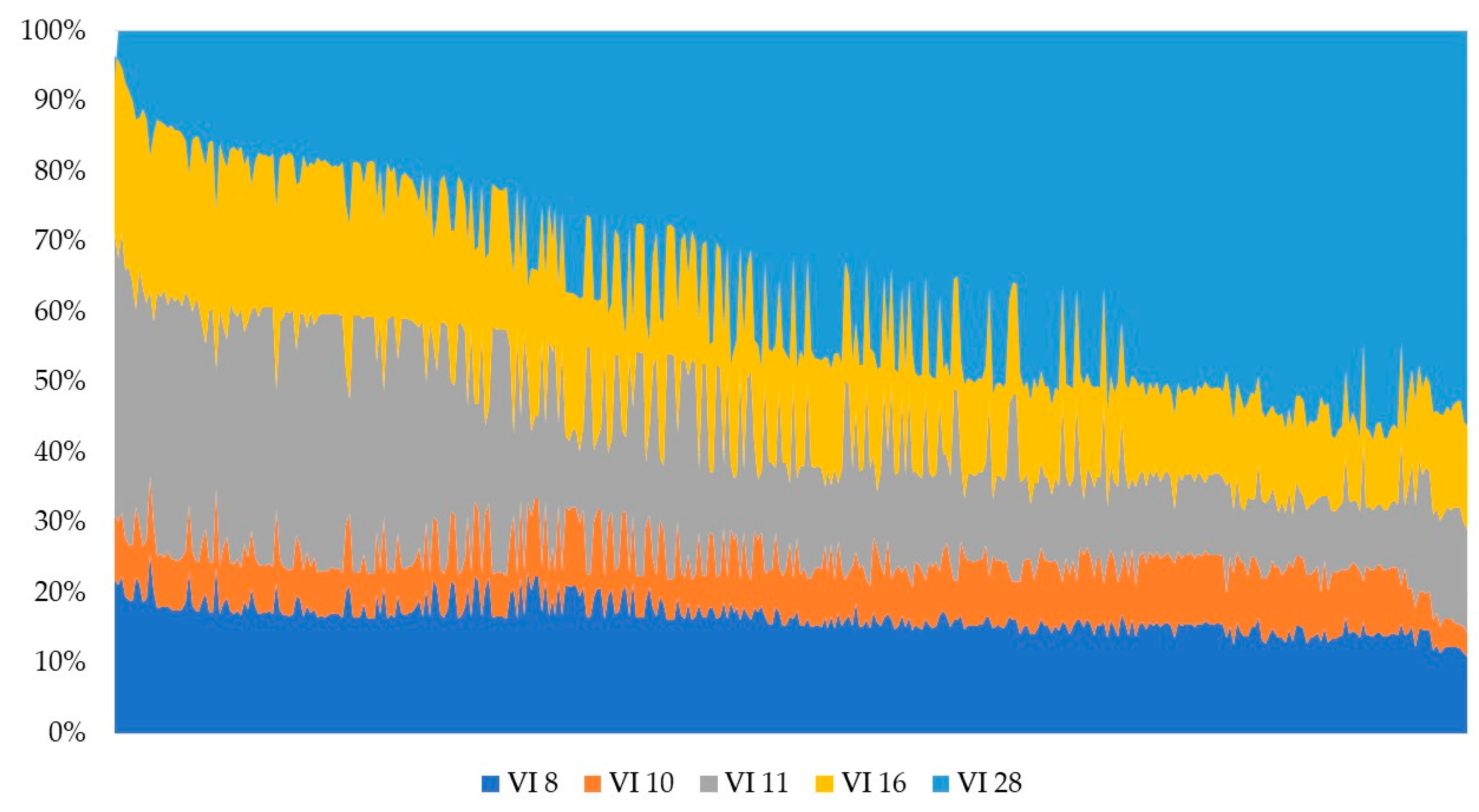
| (1) | 0.32 | 3849 | 0.00 | 1.46 | 0.37 | +VI8 ** + VI11 *** + VI16 *** + VI28 *** |
| (2) | 0.31 | 3856 | 0.00 | 1.59 | 0.69 | −VI5 + VI11 *** + VI16 *** + VI28 *** |
| (3) | 0.31 | 3856 | 0.00 | 1.11 | 0.47 | +VI10 +VI11 *** + VI16 *** + VI28 *** |
| (4) | 0.32 | 3850 | 0.00 | 1.51 | 0.40 | +VI8 ** + VI10 + VI11 *** + VI16 *** + VI28 *** |
| (5) | 0.32 | 3860 | 0.00 | 5.83 | 0.99 | −VI1 ** − VI2 + VI3 − VI4 − VI5 + VI8 ** + VI10 * VI11 *** − VI12 + VI16 *** + VI17 + VI28 *** + VI33 − VE8 * + VE19 |
| Variable | Coefficient | Std. Error | t-Statistic | Probability | Robust_SE | Robust_t | Robust_Pr | VIF |
|---|---|---|---|---|---|---|---|---|
| Intercept | −33.16 | 5.171 | −6.41 | 0.000000 * | 7.38 | −4.49 | 0.000012 * | ------- |
| VI8 | 5.44 | 1.717 | 3.17 | 0.001659 * | 2.40 | 2.27 | 0.023983 * | 1.46 |
| VI11 | 6.00 | 1.554 | 3.86 | 0.000140 * | 2.26 | 2.66 | 0.008137 * | 1.09 |
| VI16 | 5.15 | 1.504 | 3.43 | 0.000694 * | 1.38 | 3.75 | 0.000219 * | 1.18 |
| VI28 | 10.70 | 1.535 | 6.97 | 0.000000 * | 1.84 | 5.81 | 0.000000 * | 1.33 |
| Variable | Coefficient | Std. Error | t-Statistic | Probability | Robust_SE | Robust_t | Robust_Pr | VIF |
|---|---|---|---|---|---|---|---|---|
| Intercept | −36.82 | 5.985 | −6.15 | 0.000000 * | 8.34 | −4.41 | 0.000016 * | ------- |
| VI8 | 5.06 | 1.745 | 2.90 | 0.003916 * | 2.38 | 2.13 | 0.033719 * | 1.51 |
| VI10 | 2.18 | 1.797 | 1.21 | 0.225489 | 1.90 | 1.15 | 0.251148 | 1.05 |
| VI11 | 6.25 | 1.566 | 3.99 | 0.000087 * | 2.30 | 2.72 | 0.006785 * | 1.10 |
| VI16 | 5.16 | 1.503 | 3.43 | 0.000679 * | 1.38 | 3.73 | 0.000231 * | 1.18 |
| VI28 | 10.70 | 1.535 | 6.97 | 0.000000 * | 1.85 | 5.77 | 0.000000 * | 1.33 |
| Parameters | Conceptualization of Distance | ||
|---|---|---|---|
| AICc | BP Neighbors | CV | |
| Residuals square | 403,427 | 174 | 435,921 |
| Effective number | 25.9 | 5.5 | 12.2 |
| Sigma | 33.4 | 8.4 | 34.1 |
| AICc | 3841.8 | 118.3 | 3848.9 |
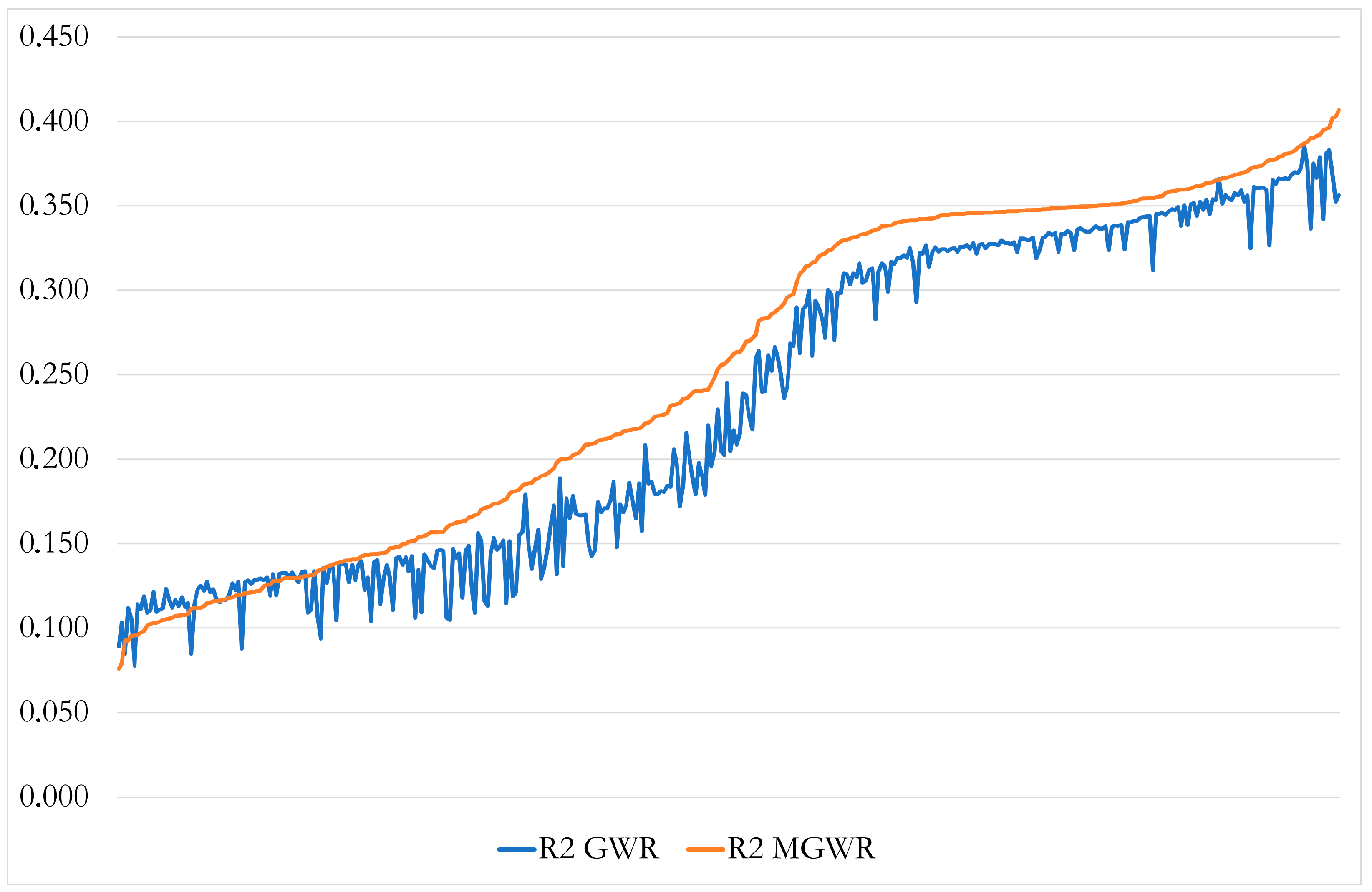
| R2 | 0.394 | 0.961 | 0.354 |
| R2 adjusted | 0.353 | 0.890 | 0.326 |
| Model configuration | Dependent variable: Rural lodging places | Independent variables: VI8–VI10–VI11–VI16–VI28 | |
| Places | Places | ||||||||
|---|---|---|---|---|---|---|---|---|---|
| Municipality | R2 | Real | Dear | Waste | Municipality | R2 | Real | Dear | Waste |
| Viandar de la Vera | 0.35 | 0 | 91 | −91 | Jaraíz de la Vera | 0.34 | 148 | 71 | 77 |
| Gargantilla | 0.33 | 8 | 92 | −84 | Acebo | 0.32 | 143 | 66 | 77 |
| Piornal | 0.34 | 5 | 84 | −79 | Burguillos del Cerro | 0.15 | 106 | 23 | 83 |
| Guijo de Santa Bárbara | 0.35 | 20 | 98 | −78 | Villanueva de la Vera | 0.35 | 180 | 91 | 89 |
| Talaveruela de la Vera | 0.35 | 10 | 85 | −75 | Jerte | 0.34 | 206 | 117 | 89 |
| Segura de Toro | 0.33 | 22 | 92 | −70 | Baños de Montemayor | 0.34 | 157 | 67 | 90 |
| Valdastillas | 0.34 | 18 | 83 | −65 | Alange | 0.11 | 104 | 8 | 96 |
| Rebollar | 0.34 | 16 | 80 | −64 | Pinofranqueado | 0.33 | 168 | 61 | 107 |
| Plasencia | 0.33 | 19 | 77 | −58 | Montánchez | 0.11 | 133 | 26 | 107 |
| Descargamaría | 0.33 | 8 | 64 | −56 | Torrejón el Rubio | 0.30 | 137 | 19 | 118 |
| Abadía | 0.33 | 0 | 56 | −56 | Valencia de Alcantara | 0.37 | 250 | 104 | 146 |
| La Garganta | 0.34 | 8 | 62 | −54 | Navaconcejo | 0.34 | 294 | 124 | 170 |
| Cabrero | 0.34 | 6 | 57 | −51 | Hervás | 0.34 | 269 | 93 | 176 |
| Jarilla | 0.33 | 18 | 68 | −50 | Jarandilla de la Vera | 0.35 | 268 | 90 | 178 |
| Variable | Est. | SE | t(Est/SE) | p-Value |
|---|---|---|---|---|
| Intercept | 0.000 | 0.042 | 0.000 | 1.000 |
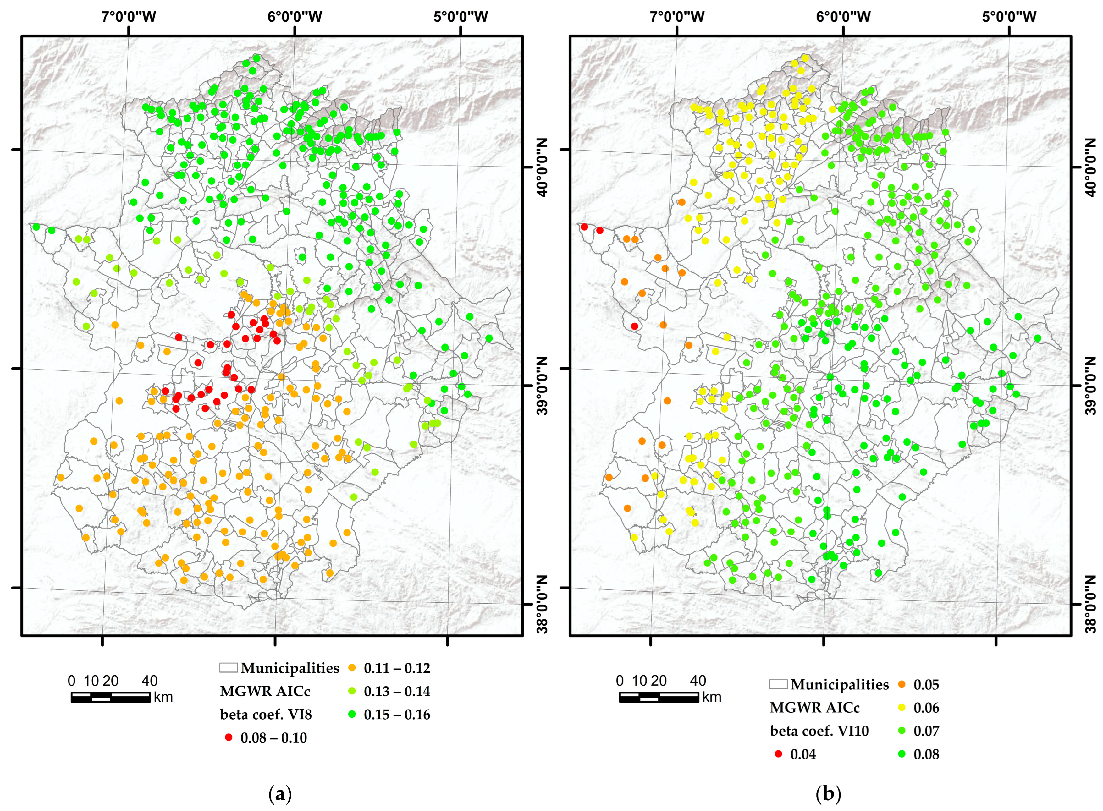
| VI8 | 0.149 | 0.051 | 2.903 | 0.004 |
| VI10 | 0.052 | 0.043 | 1.214 | 0.225 |
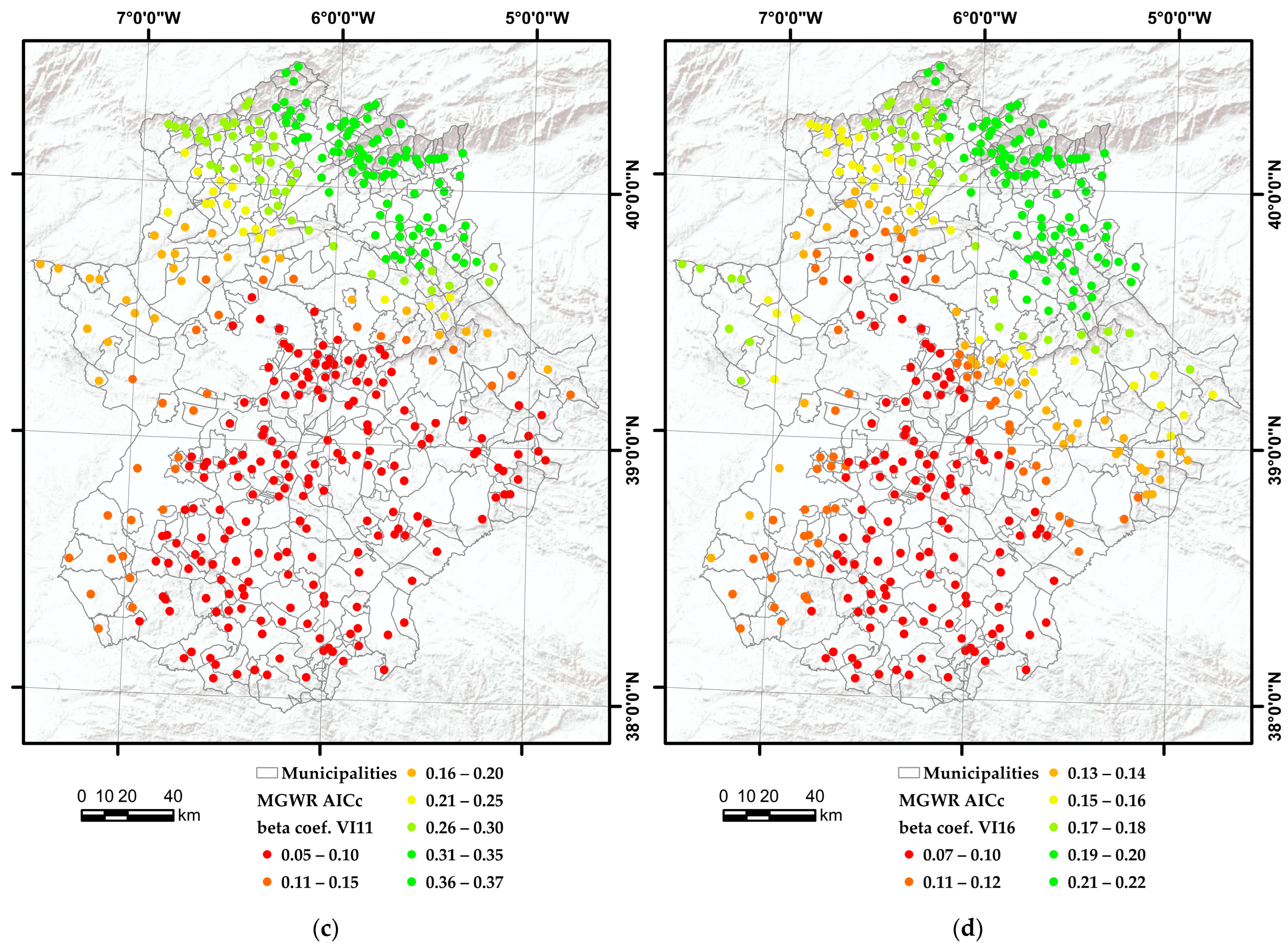
| VI11 | 0.176 | 0.044 | 3.990 | 0.000 |
| VI16 | 0.156 | 0.045 | 3.432 | 0.001 |
| VI28 | 0.336 | 0.048 | 6.972 | 0.000 |
Disclaimer/Publisher’s Note: The statements, opinions and data contained in all publications are solely those of the individual author(s) and contributor(s) and not of MDPI and/or the editor(s). MDPI and/or the editor(s) disclaim responsibility for any injury to people or property resulting from any ideas, methods, instructions or products referred to in the content. |
© 2023 by the authors. Licensee MDPI, Basel, Switzerland. This article is an open access article distributed under the terms and conditions of the Creative Commons Attribution (CC BY) license (https://creativecommons.org/licenses/by/4.0/).
Share and Cite
Sánchez-Martín, J.M.; Hernández-Carretero, A.M.; Rengifo-Gallego, J.I.; García-Berzosa, M.J.; Martín-Delgado, L.M. Modeling the Potential for Rural Tourism Development via GWR and MGWR in the Context of the Analysis of the Rural Lodging Supply in Extremadura, Spain. Systems 2023, 11, 236. https://doi.org/10.3390/systems11050236
Sánchez-Martín JM, Hernández-Carretero AM, Rengifo-Gallego JI, García-Berzosa MJ, Martín-Delgado LM. Modeling the Potential for Rural Tourism Development via GWR and MGWR in the Context of the Analysis of the Rural Lodging Supply in Extremadura, Spain. Systems. 2023; 11(5):236. https://doi.org/10.3390/systems11050236
Chicago/Turabian StyleSánchez-Martín, José Manuel, Ana María Hernández-Carretero, Juan Ignacio Rengifo-Gallego, María José García-Berzosa, and Luz María Martín-Delgado. 2023. "Modeling the Potential for Rural Tourism Development via GWR and MGWR in the Context of the Analysis of the Rural Lodging Supply in Extremadura, Spain" Systems 11, no. 5: 236. https://doi.org/10.3390/systems11050236