

Development of a Hybrid Support Vector Machine with Grey Wolf Optimization Algorithm for Detection of the Solar Power Plants Anomalies

Abstract
:1. Introduction
- This study will investigate various anomaly detection models and conduct comparison tests to evaluate their precision and performance with optimized hyperparameters.
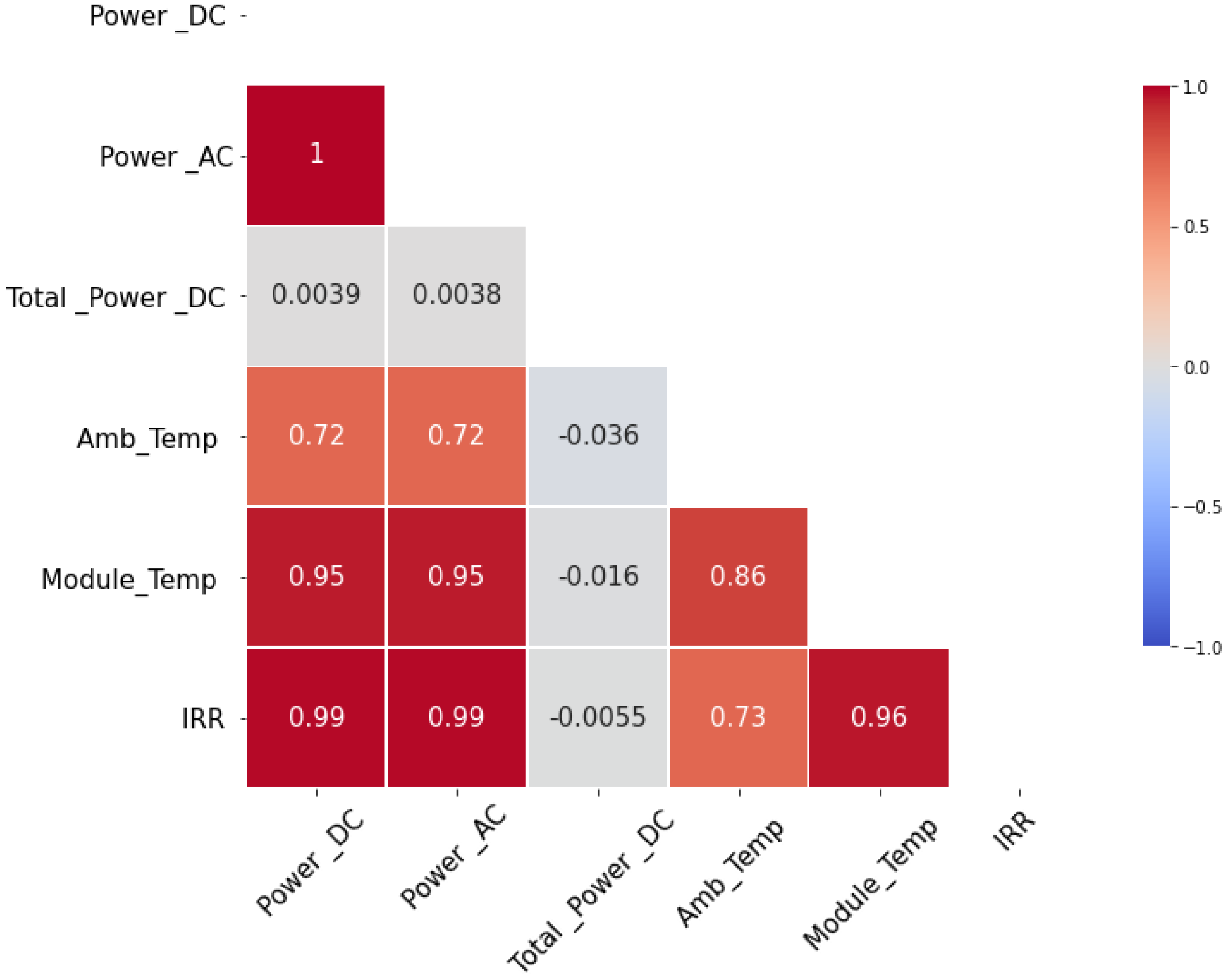
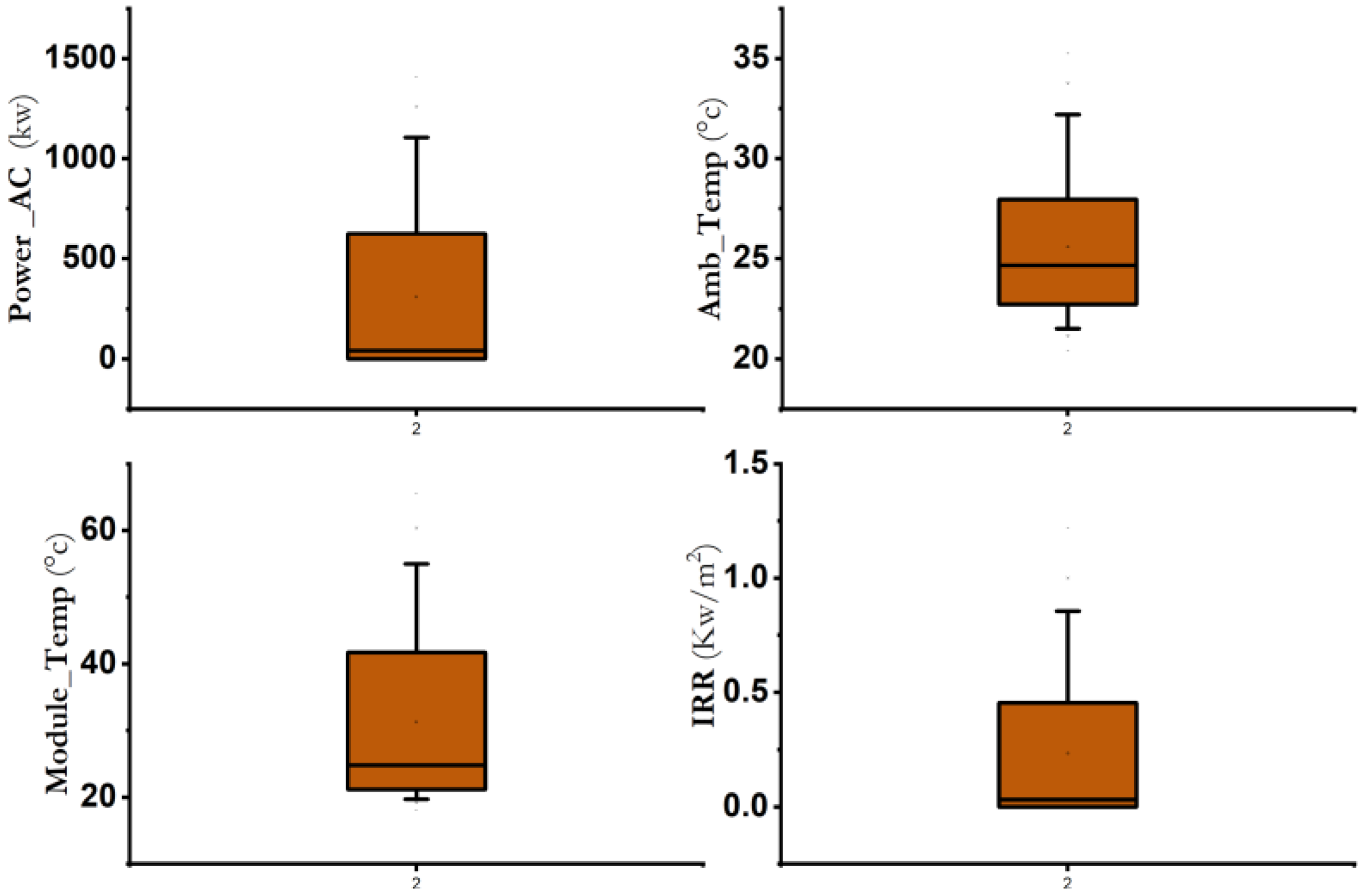
- This study aims to identify and categorize external and internal factors (AC and DC powers were an example of internal factors that may result in anomalies, while the ambient, module, and irradiation temperatures were examples of external factors) that affect anomalies in PV power plants.
- The impact of external and internal factors on model accuracy and the correlation between these factors and anomaly detection.
2. Related Work
3. Materials and Methods
3.1. Theoretical Background
- A.
- Support Vector Machine
- B.
- Support Vector Machine Regression
- C.
- Support Vector Machine Classification
- D.
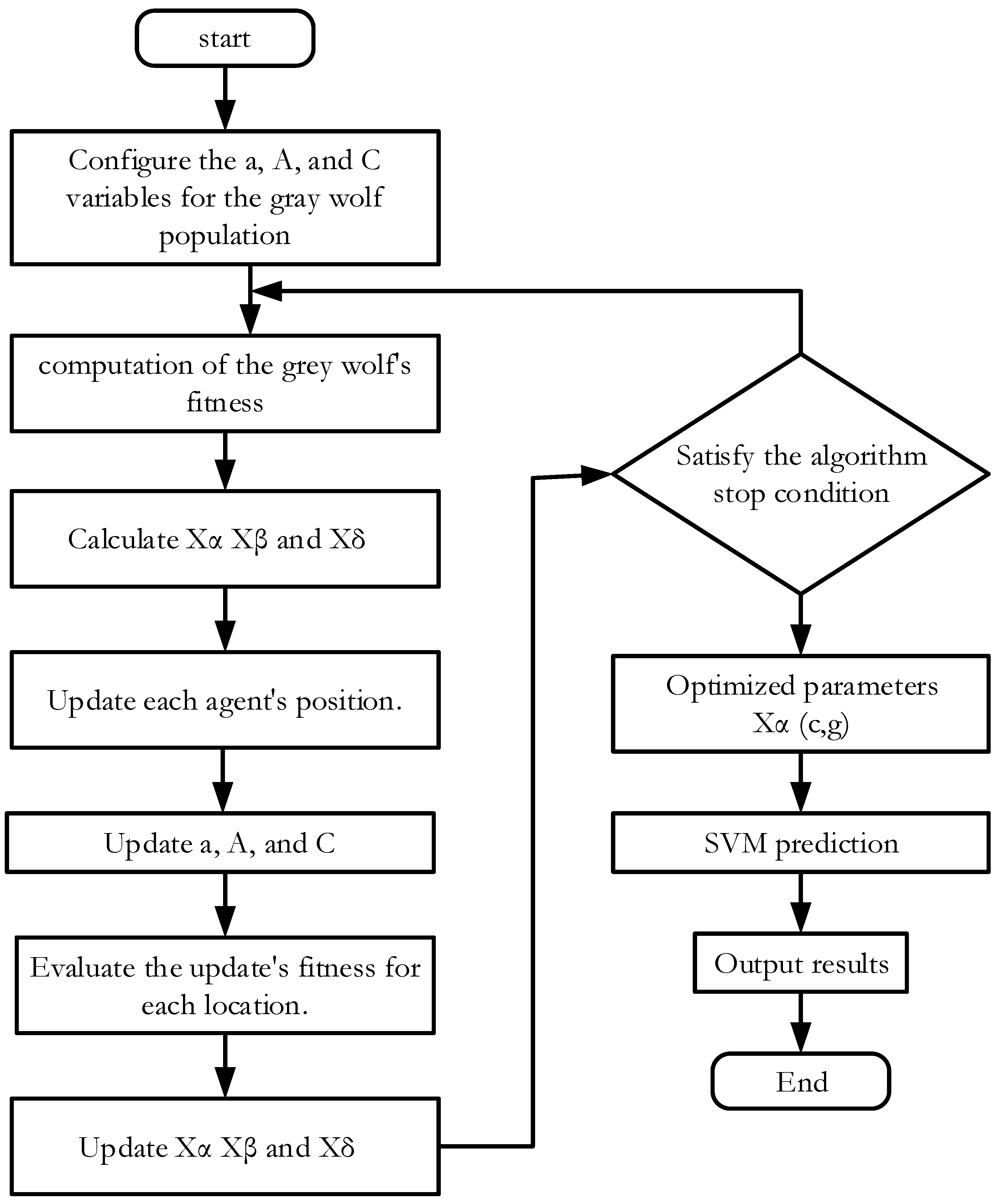
- Grey Wolf Optimizer (GWO)
- The distance separating a grey wolf and its quarry:
- 2.
- Gray wolf location update:
- 3.
- Prey position positioning:
3.2. Materials
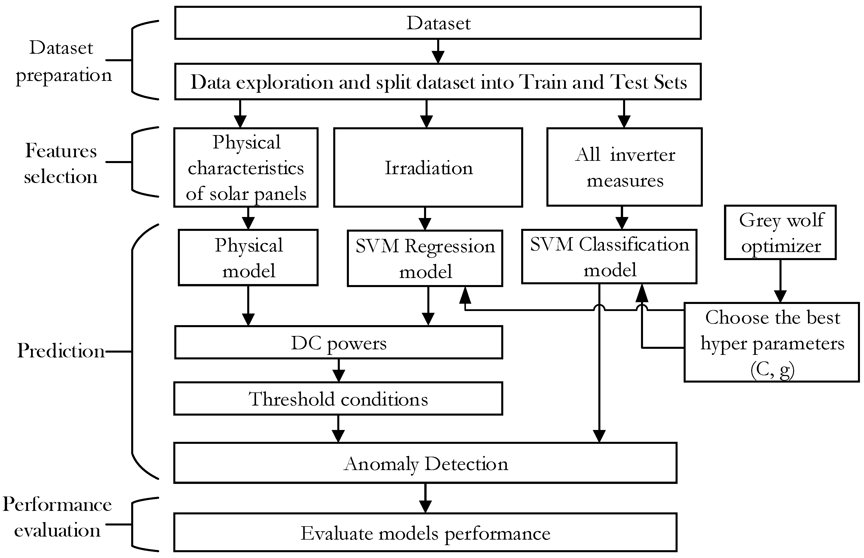
3.3. Methodology
3.3.1. Data Preparation
3.3.2. Features Selection
3.3.3. Prediction Phase
Physical Model
GWO-SVM Classification/Regression Model
3.3.4. Anomaly Prediction Decision for Models
3.3.5. Performance Evaluation
4. Experimental and Results
5. Results Discussion
6. Conclusions
Author Contributions
Funding
Data Availability Statement
Conflicts of Interest
References
- Vlaminck, M.; Heidbuchel, R.; Philips, W.; Luong, H. Region-based CNN for anomaly detection in PV power plants using aerial imagery. Sensors 2022, 22, 1244. [Google Scholar] [CrossRef] [PubMed]
- Mendes, G.; Ioakimidis, C.; Ferrão, P. On the planning and analysis of Integrated Community Energy Systems: A review and survey of available tools. Renew. Sustain. Energy Rev. 2011, 15, 4836–4854. [Google Scholar] [CrossRef]
- Ceglia, F.; Macaluso, A.; Marrasso, E.; Roselli, C.; Vanoli, L. Energy, environmental, and economic analyses of geothermal polygeneration system using dynamic simulations. Energies 2020, 13, 4603. [Google Scholar] [CrossRef]
- Lucarelli, A.; Berg, O. City branding: A state-of-the-art review of the research domain. J. Place Manag. Dev. 2011, 4, 9–27. [Google Scholar] [CrossRef]
- Andersson, I. Placing place branding: An analysis of an emerging research field in human geography. Geogr. Tidsskr. J. Geogr. 2014, 114, 143–155. [Google Scholar] [CrossRef]
- Ko, C.-C.; Liu, C.-Y.; Zhou, J.; Chen, Z.-Y. Analysis of subsidy strategy for sustainable development of environmental protection policy. IOP Conf. Ser. Earth Environ. Sci. 2019, 349, 012018. [Google Scholar] [CrossRef]
- Wei, Y.-M.; Chen, K.; Kang, J.-N.; Chen, W.; Wang, X.-Y.; Zhang, X. Policy and management of carbon peaking and carbon neutrality: A literature review. Engineering 2022, 14, 52–63. [Google Scholar] [CrossRef]
- Li, L.; Wang, Z.; Zhang, T. GBH-YOLOv5: Ghost Convolution with BottleneckCSP and Tiny Target Prediction Head Incorporating YOLOv5 for PV Panel Defect Detection. Electronics 2023, 12, 561. [Google Scholar] [CrossRef]
- Lin, L.-S.; Chen, Z.-Y.; Wang, Y.; Jiang, L.-W. Improving Anomaly Detection in IoT-Based Solar Energy System Using SMOTE-PSO and SVM Model. In Machine Learning and Artificial Intelligence; IOS Press: Cambridge, MA, USA, 2022; pp. 123–131. [Google Scholar]
- Meribout, M.; Tiwari, V.K.; Herrera, J.; Baobaid, A.N.M.A. Solar Panel Inspection Techniques and Prospects. Measurement 2023, 209, 112466. [Google Scholar] [CrossRef]
- Almalki, F.A.; Albraikan, A.A.; Soufiene, B.O.; Ali, O. Utilizing artificial intelligence and lotus effect in an emerging intelligent drone for persevering solar panel efficiency. Wirel. Commun. Mob. Comput. 2022, 2022, 7741535. [Google Scholar] [CrossRef]
- Zeng, C.; Ye, J.; Wang, Z.; Zhao, N.; Wu, M. Cascade neural network-based joint sampling and reconstruction for image compressed sensing. Signal Image Video Process. 2022, 16, 47–54. [Google Scholar] [CrossRef]
- Rahman, M.M.; Khan, I.; Alameh, K. Potential measurement techniques for photovoltaic module failure diagnosis: A review. Renew. Sustain. Energy Rev. 2021, 151, 111532. [Google Scholar] [CrossRef]
- Hooda, N.; Azad, A.P.; Kumar, P.; Saurav, K.; Arya, V.; Petra, M.I. PV power predictors for condition monitoring. In Proceedings of the 2016 IEEE International Conference on Smart Grid Communications (SmartGridComm), Sydney, Australia, 6–9 November 2016; pp. 212–217. [Google Scholar] [CrossRef]
- Kurukuru, V.S.B.; Haque, A.; Tripathy, A.K.; Khan, M.A. Machine learning framework for photovoltaic module defect detection with infrared images. Int. J. Syst. Assur. Eng. Manag. 2022, 13, 1771–1787. [Google Scholar] [CrossRef]
- Bu, C.; Liu, T.; Li, R.; Shen, R.; Zhao, B.; Tang, Q. Electrical Pulsed Infrared Thermography and supervised learning for PV cells defects detection. Sol. Energy Mater. Sol. Cells 2022, 237, 111561. [Google Scholar] [CrossRef]
- Aouat, S.; Ait-hammi, I.; Hamouchene, I. A new approach for texture segmentation based on the Gray Level Co-occurrence Matrix. Multimed. Tools Appl. 2021, 80, 24027–24052. [Google Scholar] [CrossRef]
- Mantel, C.; Villebro, F.; Benatto, G.A.D.R.; Parikh, H.R.; Wendlandt, S.; Hossain, K.; Poulsen, P.B.; Spataru, S.; Séra, D.; Forchhammer, S. Machine learning prediction of defect types for electroluminescence images of photovoltaic panels. Appl. Mach. Learn. 2019, 11139, 1113904. [Google Scholar]
- Jumaboev, S.; Jurakuziev, D.; Lee, M. Photovoltaics plant fault detection using deep learning techniques. Remote Sens. 2022, 14, 3728. [Google Scholar] [CrossRef]
- Lu, F.; Niu, R.; Zhang, Z.; Guo, L.; Chen, J. A generative adversarial network-based fault detection approach for photovoltaic panel. Appl. Sci. 2022, 12, 1789. [Google Scholar] [CrossRef]
- Elsheikh, A.H.; Katekar, V.; Muskens, O.L.; Deshmukh, S.S.; Elaziz, M.A.; Dabour, S.M. Utilization of LSTM neural network for water production forecasting of a stepped solar still with a corrugated absorber plate. Process Saf. Environ. Prot. 2021, 148, 273–282. [Google Scholar] [CrossRef]
- Elsheikh, A.H.; Panchal, H.; Ahmadein, M.; Mosleh, A.O.; Sadasivuni, K.K.; Alsaleh, N.A. Productivity forecasting of solar distiller integrated with evacuated tubes and external condenser using artificial intelligence model and moth-flame optimizer. Case Stud. Therm. Eng. 2021, 28, 101671. [Google Scholar] [CrossRef]
- Ibrahim, M.; Alsheikh, A.; Al-Hindawi, Q.; Al-Dahidi, S.; ElMoaqet, H. Short-time wind speed forecast using artificial learning-based algorithms. Comput. Intell. Neurosci. 2020, 2020, 8439719. [Google Scholar] [CrossRef] [PubMed]
- Deif, M.A.; Attar, H.; Amer, A.; Elhaty, I.A.; Khosravi, M.R.; Solyman, A.A.A. Diagnosis of Oral Squamous Cell Carcinoma Using Deep Neural Networks and Binary Particle Swarm Optimization on Histopathological Images: An AIoMT Approach. Comput. Intell. Neurosci. 2022, 2022, 6364102. [Google Scholar] [CrossRef] [PubMed]
- Aslam, S.; Herodotou, H.; Mohsin, S.M.; Javaid, N.; Ashraf, N.; Aslam, S. A survey on deep learning methods for power load and renewable energy forecasting in smart microgrids. Renew. Sustain. Energy Rev. 2021, 144, 110992. [Google Scholar] [CrossRef]
- Ibrahim, M.; Alsheikh, A.; Awaysheh, F.M.; Alshehri, M.D. Machine learning schemes for anomaly detection in solar power plants. Energies 2022, 15, 1082. [Google Scholar] [CrossRef]
- Branco, P.; Gonçalves, F.; Costa, A.C. Tailored algorithms for anomaly detection in photovoltaic systems. Energies 2020, 13, 225. [Google Scholar] [CrossRef]
- Deif, M.A.; Solyman, A.A.A.; Hammam, R.E. ARIMA Model Estimation Based on Genetic Algorithm for COVID-19 Mortality Rates. Int. J. Inf. Technol. Decis. Mak. 2021, 20, 1775–1798. [Google Scholar] [CrossRef]
- De Benedetti, M.; Leonardi, F.; Messina, F.; Santoro, C.; Vasilakos, A. Anomaly detection and predictive maintenance for photovoltaic systems. Neurocomputing 2018, 310, 59–68. [Google Scholar] [CrossRef]
- Natarajan, K.; Bala, K.; Sampath, V. Fault detection of solar PV system using SVM and thermal image processing. Int. J. Renew. Energy Res. 2020, 10, 967–977. [Google Scholar]
- Harrou, F.; Dairi, A.; Taghezouit, B.; Sun, Y. An unsupervised monitoring procedure for detecting anomalies in photovoltaic systems using a one-class support vector machine. Sol. Energy 2019, 179, 48–58. [Google Scholar] [CrossRef]
- Feng, M.; Bashir, N.; Shenoy, P.; Irwin, D.; Kosanovic, D. Sundown: Model-driven per-panel solar anomaly detection for residential arrays. In Proceedings of the 3rd ACM SIGCAS Conference on Computing and Sustainable Societies, Guayaquil, Ecuador, 15–17 June 2020; pp. 291–295. [Google Scholar]
- Sanz-Bobi, M.A.; Roque, A.M.S.; De Marcos, A.; Bada, M. Intelligent system for a remote diagnosis of a photovoltaic solar power plant. J. Phys. Conf. Ser. 2012, 364, 012119. [Google Scholar] [CrossRef]
- Zhao, Y.; Liu, Q.; Li, D.; Kang, D.; Lv, Q.; Shang, L. Hierarchical anomaly detection and multimodal classification in large-scale photovoltaic systems. IEEE Trans. Sustain. Energy 2018, 10, 1351–1361. [Google Scholar] [CrossRef]
- Mulongo, J.; Atemkeng, M.; Ansah-Narh, T.; Rockefeller, R.; Nguegnang, G.M.; Garuti, M.A. Anomaly detection in power generation plants using machine learning and neural networks. Appl. Artif. Intell. 2020, 34, 64–79. [Google Scholar] [CrossRef]
- Benninger, M.; Hofmann, M.; Liebschner, M. Online Monitoring System for Photovoltaic Systems Using Anomaly Detection with Machine Learning. In Proceedings of the NEIS 2019 Conference on Sustainable Energy Supply and Energy Storage Systems, Hamburg, Germany, 17 February 2020; pp. 1–6. [Google Scholar]
- Benninger, M.; Hofmann, M.; Liebschner, M. Anomaly detection by comparing photovoltaic systems with machine learning methods. In Proceedings of the NEIS 2020 Conference on Sustainable Energy Supply and Energy Storage Systems Hamburg, Germany, 1 December 2020; pp. 1–6. [Google Scholar]
- Firth, S.K.; Lomas, K.J.; Rees, S.J. A simple model of PV system performance and its use in fault detection. Sol. Energy 2010, 84, 624–635. [Google Scholar] [CrossRef]
- Balzategui, J.; Eciolaza, L.; Maestro-Watson, D. Anomaly detection and automatic labeling for solar cell quality inspection based on generative adversarial network. Sensors 2021, 21, 4361. [Google Scholar] [CrossRef]
- Wang, Q.; Paynabar, K.; Pacella, M. Online automatic anomaly detection for photovoltaic systems using thermography imaging and low rank matrix decomposition. J. Qual. Technol. 2022, 54, 503–516. [Google Scholar] [CrossRef]
- Hempelmann, S.; Feng, L.; Basoglu, C.; Behrens, G.; Diehl, M.; Friedrich, W.; Brandt, S.; Pfeil, T. Evaluation of unsupervised anomaly detection approaches on photovoltaic monitoring data. In Proceedings of the 2020 47th IEEE Photovoltaic Specialists Conference (PVSC), Calgary, ON, Canada, 15 June–21 August 2020; pp. 2671–2674. [Google Scholar]
- Iyengar, S.; Lee, S.; Sheldon, D.; Shenoy, P. Solarclique: Detecting anomalies in residential solar arrays. In Proceedings of the 1st ACM SIGCAS Conference on Computing and Sustainable Societies, Menlo Park and San Jose, CA, USA, 20–22 June 2018; pp. 1–10. [Google Scholar]
- Tsai, C.-W.; Yang, C.-W.; Hsu, F.-L.; Tang, H.-M.; Fan, N.-C.; Lin, C.-Y. Anomaly Detection Mechanism for Solar Generation using Semi-supervision Learning Model. In Proceedings of the 2020 Indo--Taiwan 2nd International Conference on Computing, Analytics and Networks (Indo-Taiwan ICAN), Rajpura, India, 7–15 February 2020; pp. 9–13. [Google Scholar]
- Pereira, J.; Silveira, M. Unsupervised anomaly detection in energy time series data using variational recurrent autoencoders with attention. In Proceedings of the 2018 17th IEEE International Conference on Machine Learning and Applications (ICMLA), Orlando, FL, USA, 17–20 December 2018; pp. 1275–1282. [Google Scholar]
- Kosek, A.M.; Gehrke, O. Ensemble regression model-based anomaly detection for cyber-physical intrusion detection in smart grids. In Proceedings of the 2016 IEEE Electrical Power and Energy Conference (EPEC), Ottawa, ON, Canada, 12–14 October 2016; pp. 1–7. [Google Scholar]
- Rossi, B.; Chren, S.; Buhnova, B.; Pitner, T. Anomaly detection in smart grid data: An experience report. In Proceedings of the 2016 IEEE International Conference on Systems Man, and Cybernetics (SMC), Budapest, Hungary, 9–12 October 2016; pp. 2313–2318. [Google Scholar]
- Toshniwal, A.; Mahesh, K.; Jayashree, R. Overview of anomaly detection techniques in machine learning. In Proceedings of the 2020 Fourth International Conference on I-SMAC (IoT in Social Mobile, Analytics and Cloud) (I-SMAC), Palladam, India, 7–9 October 2020; pp. 808–815. [Google Scholar]
- Deif, M.A.; Solyman, A.A.A.; Alsharif, M.H.; Jung, S.; Hwang, E. A hybrid multi-objective optimizer-based SVM model for enhancing numerical weather prediction: A study for the Seoul metropolitan area. Sustainability 2021, 14, 296. [Google Scholar] [CrossRef]
- Hammam, R.E.; Attar, H.; Amer, A.; Issa, H.; Vourganas, I.; Solyman, A.; Venu, P.; Khosravi, M.R.; Deif, M.A. Prediction of Wear Rates of UHMWPE Bearing in Hip Joint Prosthesis with Support Vector Model and Grey Wolf Optimization. Wirel. Commun. Mob. Comput. 2022, 2022, 6548800. [Google Scholar] [CrossRef]
- Deif, M.A.; Hammam, R.E.; Solyman, A.; Alsharif, M.H.; Uthansakul, P. Automated Triage System for Intensive Care Admissions during the COVID-19 Pandemic Using Hybrid XGBoost-AHP Approach. Sensors 2021, 21, 6379. [Google Scholar] [CrossRef]
- Deif, M.A.; Hammam, R.E. Skin lesions classification based on deep learning approach. J. Clin. Eng. 2020, 45, 155–161. [Google Scholar] [CrossRef]
- Deif, M.A.; Solyman, A.A.; Kamarposhti, M.A.; Band, S.S.; Hammam, R.E. A deep bidirectional recurrent neural network for identification of SARS-CoV-2 from viral genome sequences. Math. Biosci. Eng. AIMS-Press 2021, 18, 8933–8950. [Google Scholar] [CrossRef]
- Deif, M.A.; Attar, H.; Amer, A.; Issa, H.; Khosravi, M.R.; Solyman, A.A.A. A New Feature Selection Method Based on Hybrid Approach for Colorectal Cancer Histology Classification. Wirel. Commun. Mob. Comput. 2022, 2022, 7614264. [Google Scholar] [CrossRef]
- Zamfirache, I.A.; Precup, R.-E.; Roman, R.-C.; Petriu, E.M. Policy iteration reinforcement learning-based control using a grey wolf optimizer algorithm. Inf. Sci. 2022, 585, 162–175. [Google Scholar] [CrossRef]
- Kannal, A. Solar Power Generation Data. Kaggle.com. 2020. Available online: https//www.kaggle.com/anikannal/solar-powergeneration-data (accessed on 30 January 2022).


| Variable Type | Variable Name | Variable Abbreviation (Unit) | Variable Description |
|---|---|---|---|
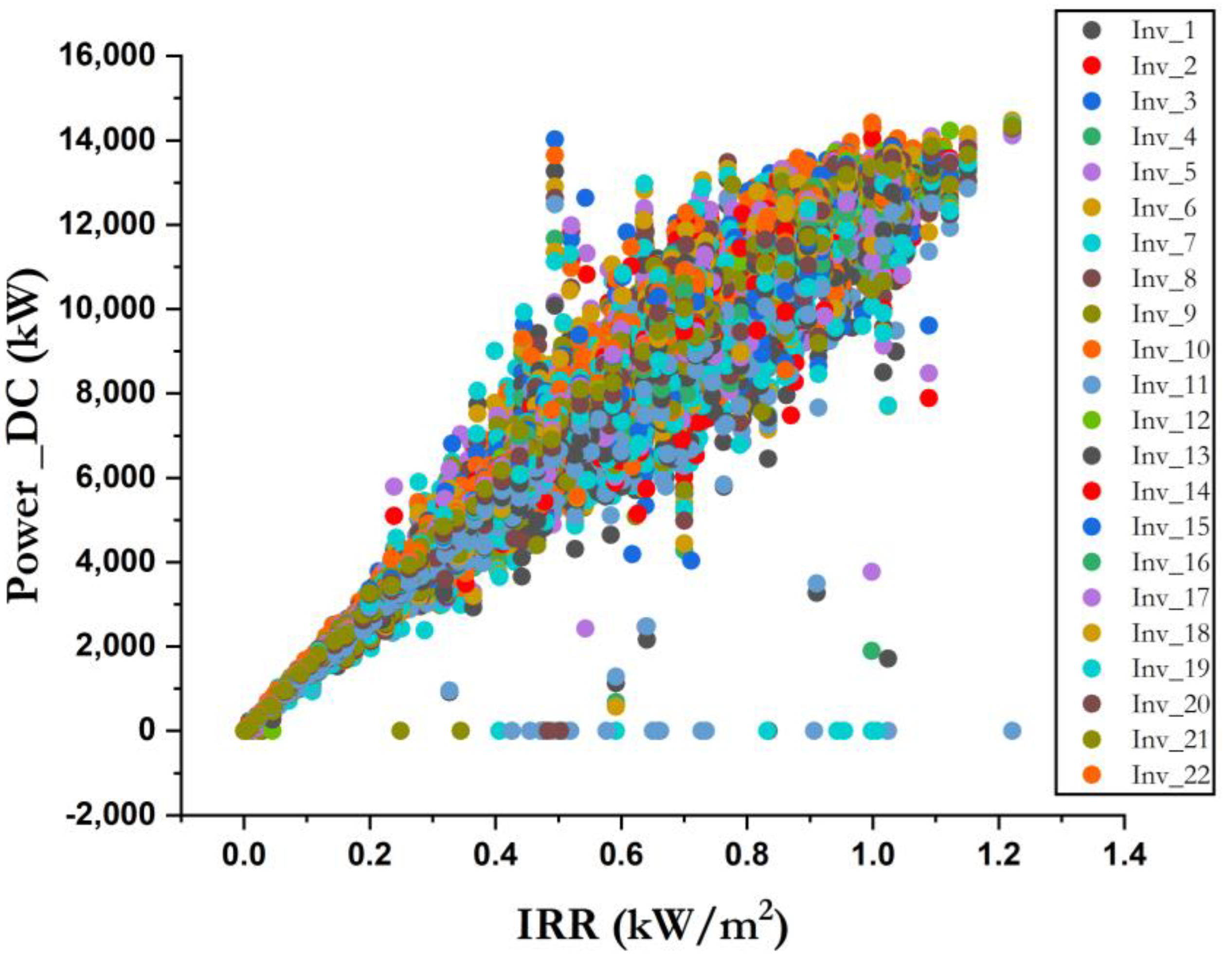
| Internal factor | DC power | Power_DC (kW) | The DC power produced by the inverter |
| AC power | Power_AC (kW) | The AC power produced by the inverter | |
| Total yield | Total_power_DC (kW) | The total DC power output from the inverter over a period of time. | |
| External factors | Solar irradiance | IRR (kW/m2) | The intensity of the electromagnetic radiation emitted by the sun per unit area |
| Ambient temperature | Amb_Temp (°C) | The temperature around the solar power plant | |
| Solar panel temperature | Module_Temp (°C) | The temperature indication for the solar module is measured by attaching a sensor to the panel. |
| Optimizer Name | Parameter | Value |
|---|---|---|
| GWO | A | Min = 0 and max = 2 |
| Number of agents | 100 | |
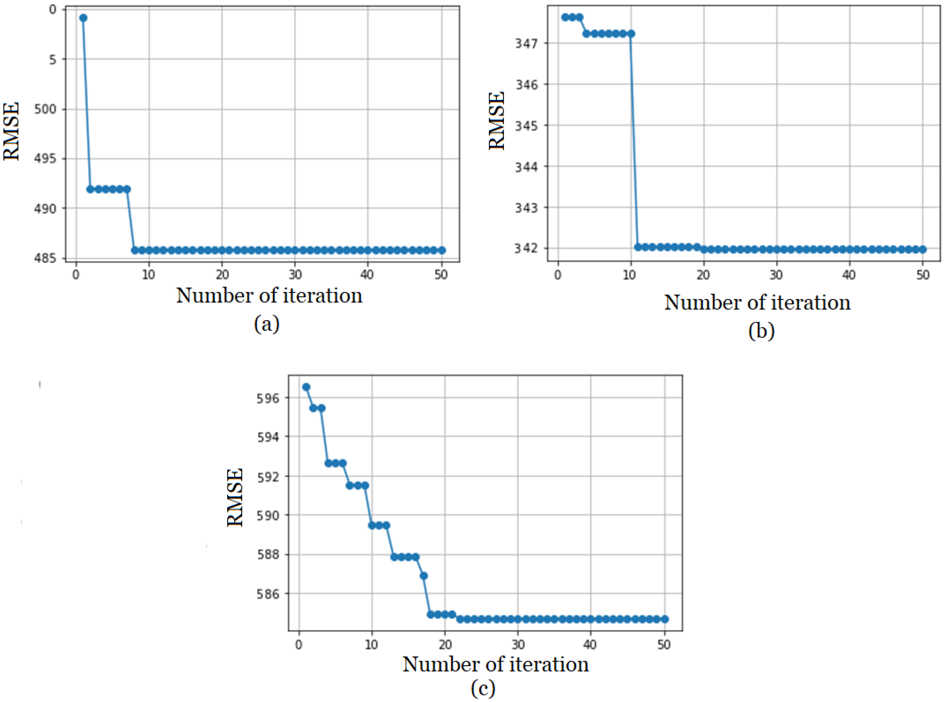
| Iterations number | 50 | |
| GS and RS | C = Linear | Min = 0.001 and max = 10,000 |
| G = Linear, RBF, sigmoid | Min = 0.001 and max = 10,000 |
| Model | RMSE |
|---|---|
| RS_SVM | 532.47 |
| SVM_R | 415.98 |
| GS_SVM | 400.83 |
| GWO-SVM_R | 318.04 |
| Model | Sensitivity | Specificity |
|---|---|---|
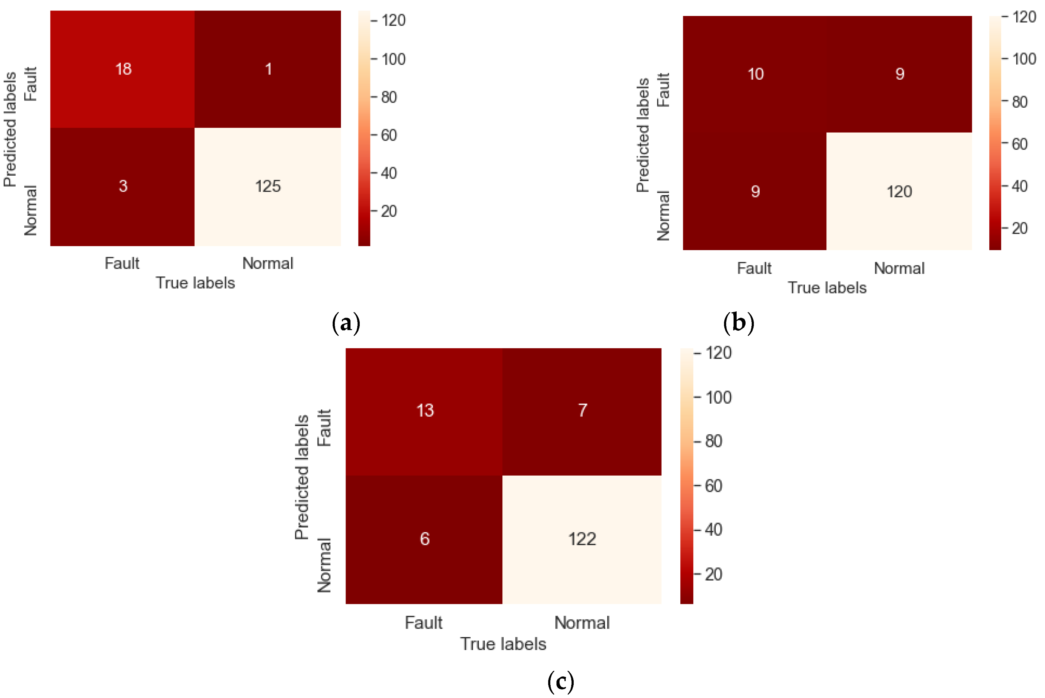
| SVM-GW_C | 85.71% | 99.21% |
| SVM-GW_R | 68.42% | 94.57% |
| Physical model | 52.63% | 93.02% |
| Model | Accuracy (%) | Sensitivity (%) | Specificity (%) |
|---|---|---|---|
| SVM-GW_C | 97.28 | 85.71% | 99.21% |
| Reference model | 89.63 | 94.32 | 100% |
Disclaimer/Publisher’s Note: The statements, opinions and data contained in all publications are solely those of the individual author(s) and contributor(s) and not of MDPI and/or the editor(s). MDPI and/or the editor(s) disclaim responsibility for any injury to people or property resulting from any ideas, methods, instructions or products referred to in the content. |
© 2023 by the authors. Licensee MDPI, Basel, Switzerland. This article is an open access article distributed under the terms and conditions of the Creative Commons Attribution (CC BY) license (https://creativecommons.org/licenses/by/4.0/).
Share and Cite
Ahmed, Q.I.; Attar, H.; Amer, A.; Deif, M.A.; Solyman, A.A.A. Development of a Hybrid Support Vector Machine with Grey Wolf Optimization Algorithm for Detection of the Solar Power Plants Anomalies. Systems 2023, 11, 237. https://doi.org/10.3390/systems11050237
Ahmed QI, Attar H, Amer A, Deif MA, Solyman AAA. Development of a Hybrid Support Vector Machine with Grey Wolf Optimization Algorithm for Detection of the Solar Power Plants Anomalies. Systems. 2023; 11(5):237. https://doi.org/10.3390/systems11050237
Chicago/Turabian StyleAhmed, Qais Ibrahim, Hani Attar, Ayman Amer, Mohanad A. Deif, and Ahmed A. A. Solyman. 2023. "Development of a Hybrid Support Vector Machine with Grey Wolf Optimization Algorithm for Detection of the Solar Power Plants Anomalies" Systems 11, no. 5: 237. https://doi.org/10.3390/systems11050237