A Learning-Based Optimal Decision Scenario for an Inventory Problem under a Price Discount Policy

 , , ,
, , ,  and
and
Abstract
:1. Introduction
- What is the appropriate approach in a marketing scenario driven by the EOQ model where uncertain demands of the customers depend on the unit selling price?
- How does the uncertain demand pattern affect the decision-making process?
- How does the price discount facility affect the profit-optimizing policy?
- How much can the decision-maker benefit from learning by performing repetitive tasks to implement a more robust strategy to achieve his/her purpose?
- What are the immediate effects of the unit price discount policy and learning through experience on the economic order quantity model?
2. Theoretical Background
2.1. Recent Advancement in Inventory Modeling
2.2. Price Discount Policy-Based Inventory Model
2.3. Fuzzy Differential Equation in Inventory Model
2.4. Learning-Based Decision-Making Using the Inventory Model
2.5. Research Gaps and Novelty of This Paper
- Apart from the papers [49,50], we have yet to come across many works in the literature that use learning as a dense fuzzy set to define an EOQ model. The fuzzy setup in this study incorporates the concept of learning in terms of TDFS and uncertainty with related factors and variables. The TDFS theory explains how the degree of ambiguity regarding demand patterns decreases over time (because of repeated experiences with similar types of decision-making phenomena).
- The selling price has a great impact on the design of consumption. The retailers may offer a low price to boost consumer demand and thus the average turnover. However, the loosely supervised decisions to lower the selling price may cause high demand locally. Therefore, the demand is negatively proportionate to the unit retailing price.
- The demand, as well as the retail price, may not always be accurate to the retailer. As a result, we considered the unit selling price and hence the demand pattern of the customer as a triangular dense fuzzy number to maximize the average turnover.
- Another critical point is the all-units discount policy. All-unit discount facilities are crucial for competitive business because of the globalization of the marketing strategy. Until now, almost all the works [20,21,22,24,25,28,29,30] considering this fact have been completed in a crisp environment.
3. Preliminaries
4. Different Notations and Assumptions
4.1. Notations
4.2. Assumptions
- (a)
- We consider straightforward fact while formulating the demand function. The demand rate () is dependent on the unit selling price . Generally, the demand for certain commodities can be boosted by lowering the retail price. In a retail market with fluctuations in demand and the retail price, the uncertainty can be adjusted by using a fuzzy equation as follows. Thus, mathematically, the uncertain fuzzy demand can be viewed as, i.e., , where is taken as triangular dense fuzzy number, is the fixed demand, and is the coefficient of price in the demand function. We assume a decision-making phenomenon where the unit selling price becomes precise gradually due to learning experience gained through repeating the same kind of tasks. Thus, we consider the uncertain unit selling price as a triangular dense fuzzy number. As the number of repetitions increase, more information is collected, and the analysis will provide a more precise prediction, and thus, the uncertainty will start to disappear.
- (b)
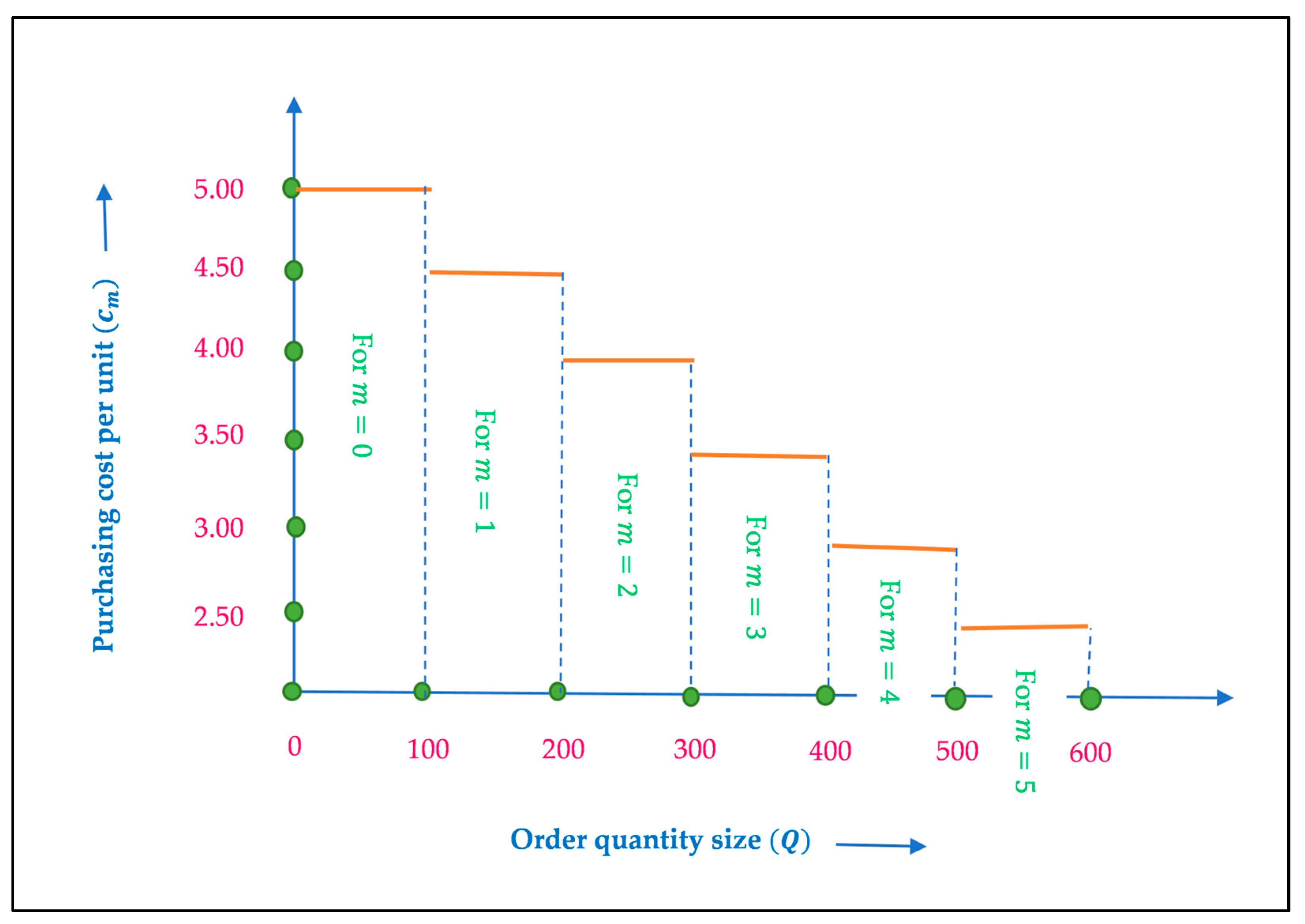
- We consider that the discount facility is available while the retailer is purchasing from a supplier. The discount is availing on the order quantity of the purchasing commodities, and the interacting situation contains impreciseness. The purchasing cost per unit decreases as the order size increases. To trace the uncertainty, we assume a fuzzy unit purchase cost as a discrete step function for the fuzzy ordering quantities as follows: , for and . In above equations, represents the number of repetitions required to lessen the fuzzy uncertainty regarding the purchasing cost per unit through repetitive tasks. In addition, represents the number of repetitions required to adjust perfect combinations of the purchasing cost and order size, since discretely related combinations of them are available in the purchasing scenario.
- (c)
- The carrying cost per unit increases as time increases, as the maintenance ability of the carrying machineries deteriorate over time. In addition, carrying costs depend on order size and thus on the purchasing cost per unit. Therefore, the holding cost is proportional the unit purchasing cost and it is also linear function of time. Thus, the unit holding cost is .
- (d)
- The lead time is zero.
- (e)
- Shortages are not allowed.
- (f)
- Replenishment is instantaneous.
5. Mathematical Modeling of the Fuzzy EOQ Model
5.1. Crisp Model
- (i)
- The replenishment cost is constant and is taken to be .
- (ii)
- Suppose the purchase cost per unit is a crisp number fitted for the ordering size (). Then, the total purchase cost for lot size is obtained as:
- (iii)
- The holding cost per unit is a function of the purchase cost per unit and time. Therefore, the total holding cost during all the retail activities is obtained as:
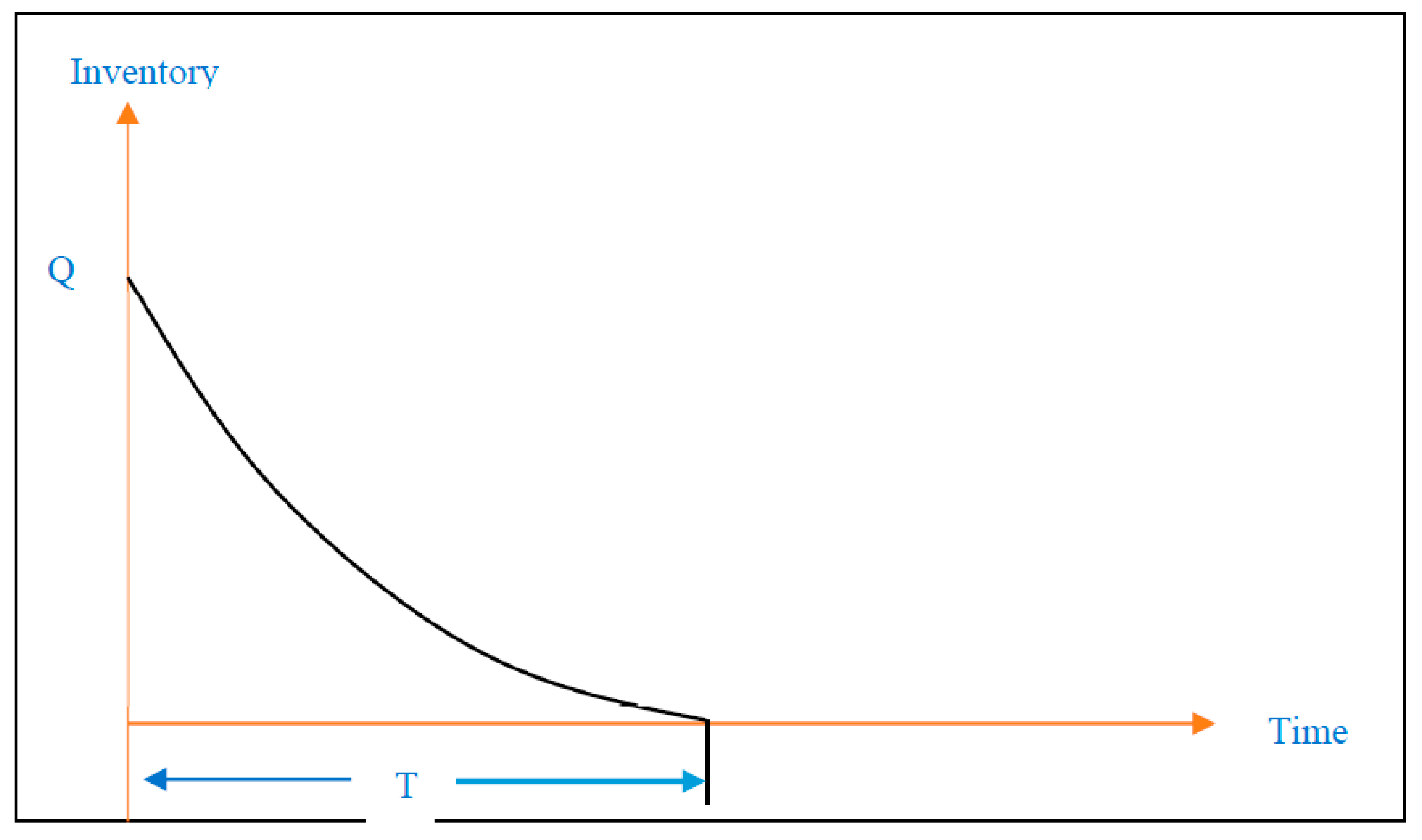
- (iv)
- Suppose the selling price per unit is also a crisp number. Then, the total earned revenue can be calculated multiplying the consumed amount of product by the selling price per unit. Therefore, the earned revenue from the retail activities is obtained as:
- (v)
- The total profit is the difference between the earned revenue and the sum of all possible costs. The total average profit is obtained dividing the total profit by the cycle time as follows:
5.2. Fuzzification of the Crisp Objective Function Implementing TDFS in Decision-Making
5.2.1. Using the Direct Index Value of Each Fuzzy Parameter (Method 1)
- (i)
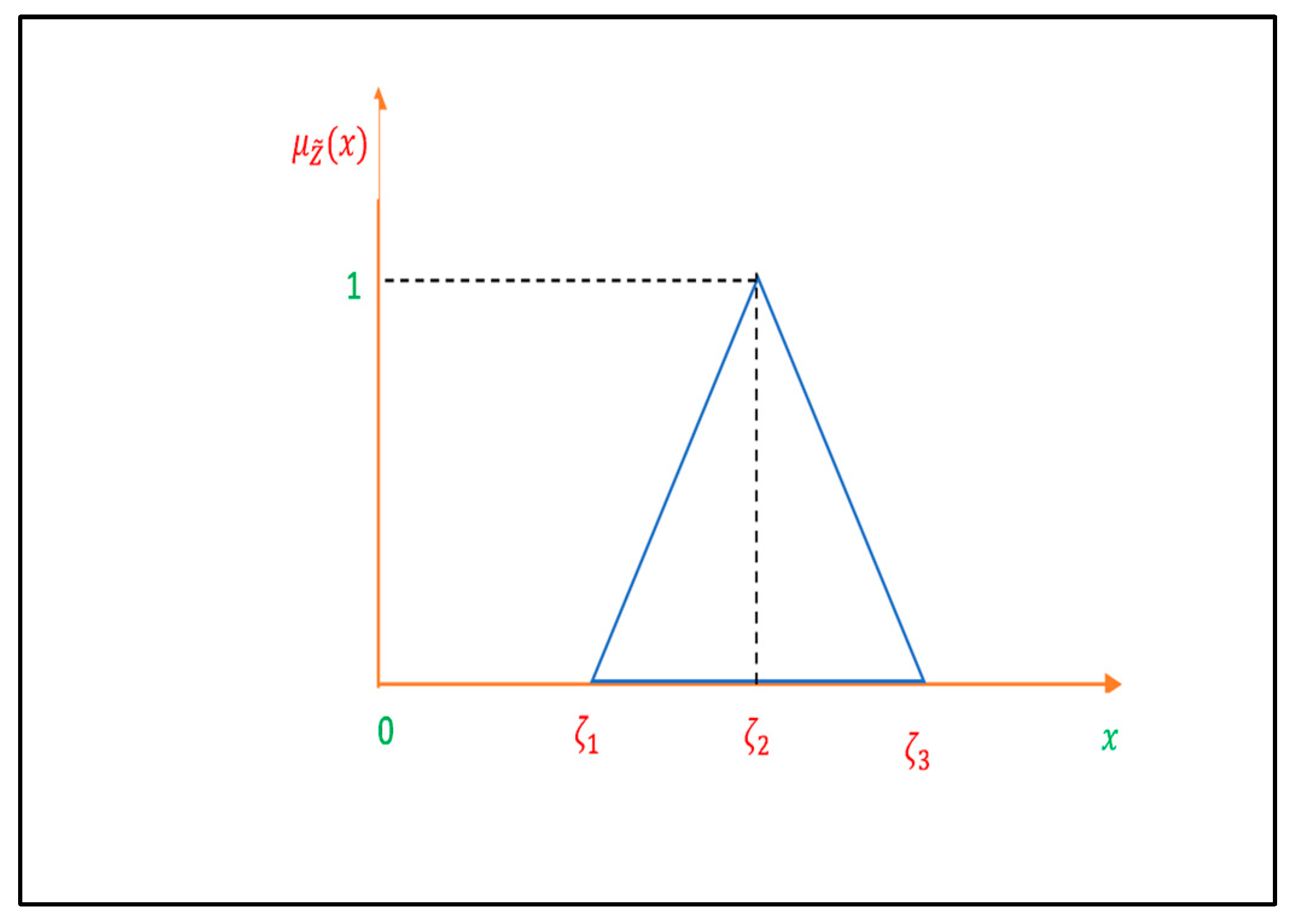
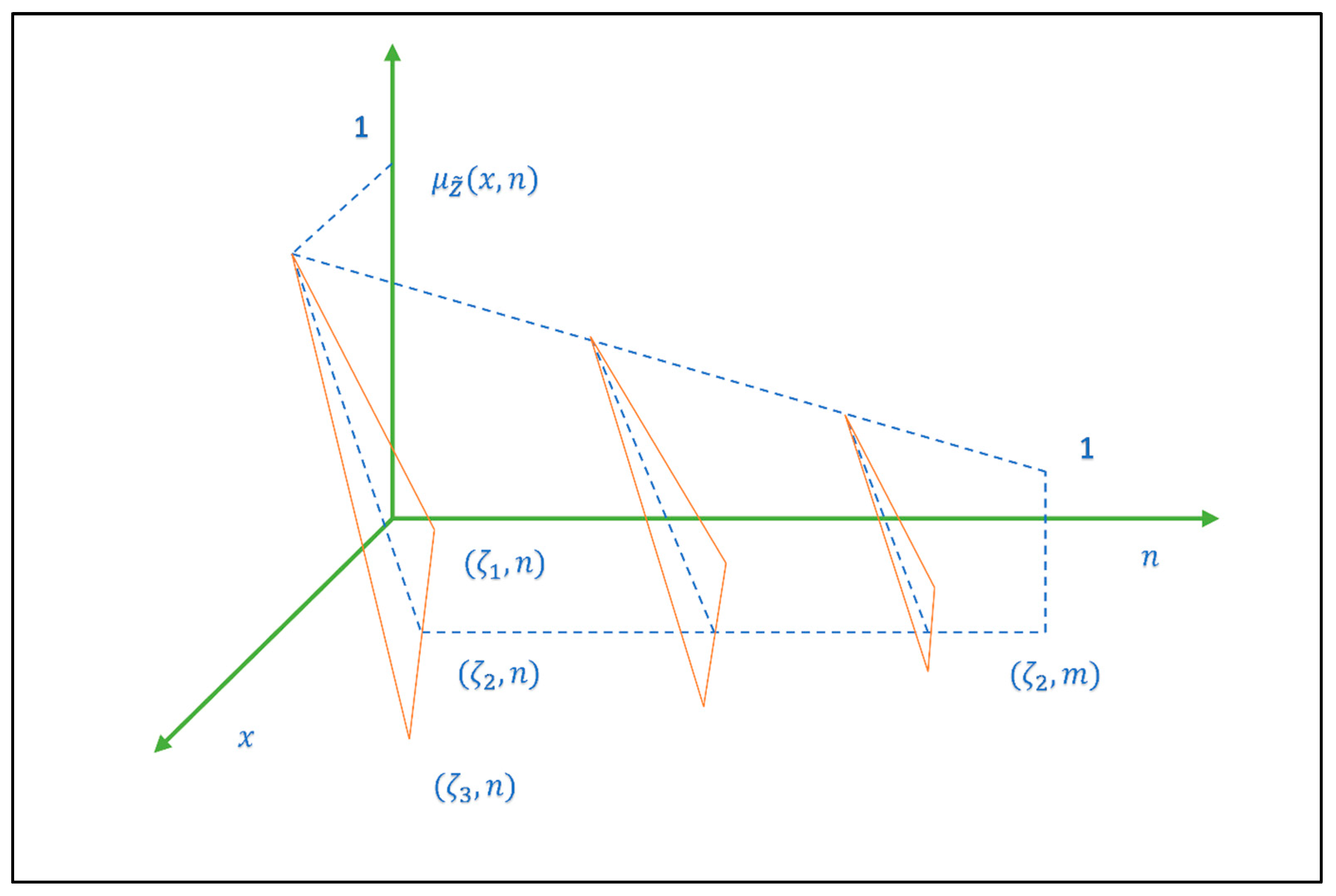
- The -cut of a TDFS is given by
- (ii)
- The -cut of a TDFS is given by
- (iii)
- The -cut of a TDFS is given by and the index value of is obtained as follows:
5.2.2. Using Fuzzy Arithmetic Operation and the Index Value Concept (Method 2)
5.3. Fuzzy Differential Equation Approach
- Case I: when is (1)-gH differentiable.
- Case II: when is (2)-gH differentiable.
6. Numerical Exploration
6.1. Solution Algorithm
| Algorithm 1. Algorithm for optimal feasible solution in different scenarios. | |
| 1: | Inputs: the value of the parameters . |
| 2: | Outputs: total average profit (TAP), optimal order size (Q), and total cycle length (T). |
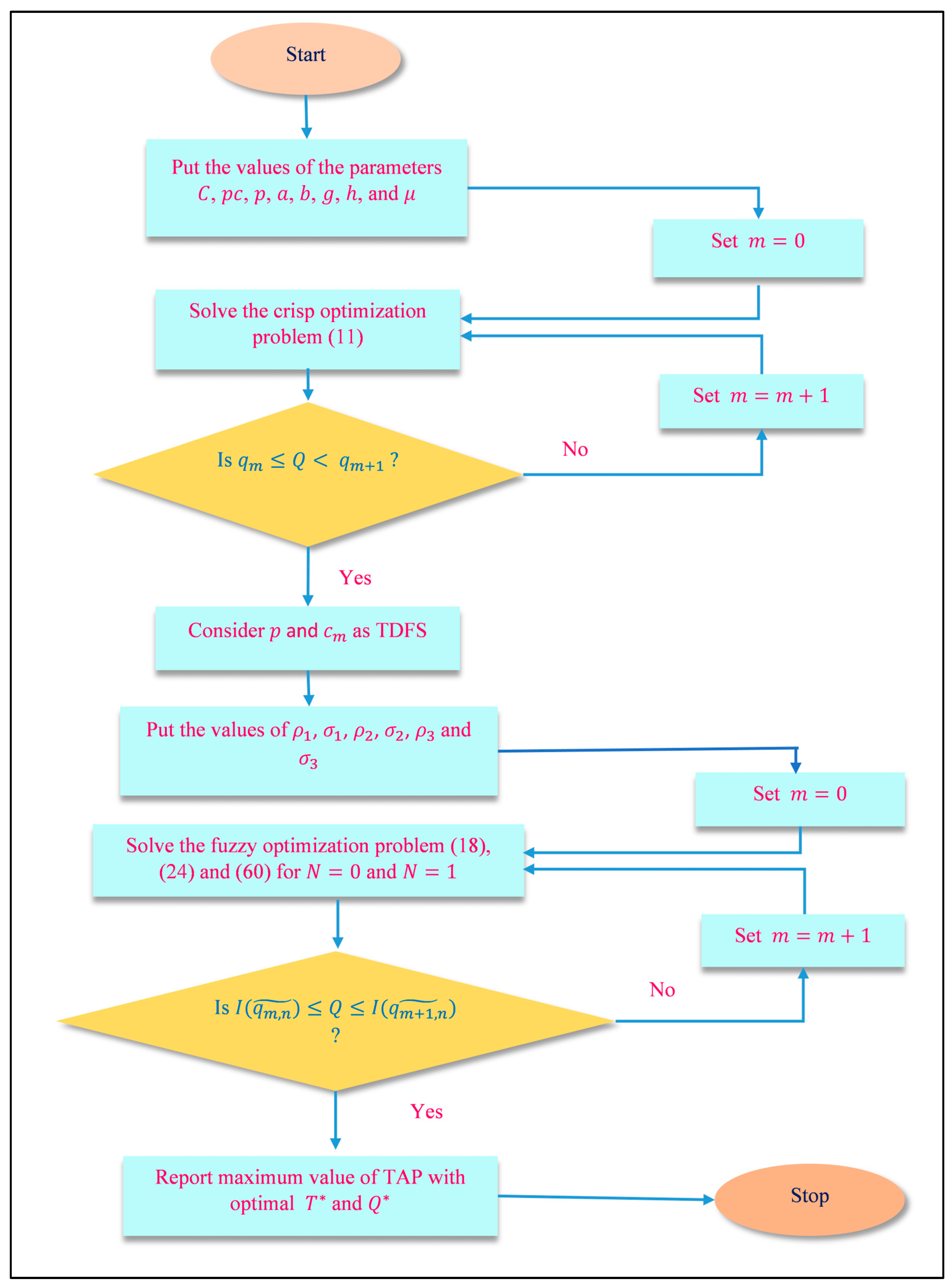
| 3: | Step 1. Set . |
| 4: | Step 2. Solve the crisp optimization problem (11). |
| 5: | Step 3. If , this solution is infeasible. Set and go to step 2. Otherwise, go to step 4. |
| 6: | Step 4. If , this solution is feasible. Set , and for a crisp problem and go to step 5. |
| 7: | Step 5. Consider the unit selling price and unit purchase cos as a triangular dense fuzzy number. |
| 8: | Step 6. Input . |
| 9: | Step 7. Set . |
| 10: | Step 8. Solve the fuzzy optimization problem (18), (24), and (60) for N = 0 and N = 1. |
| 11: | Step 9. If , then the solution is feasible. Go to step 11. Otherwise, go to step 10. |
| 12: | Step 10. Set , and go to step 7. |
| 13: | Step 11. Obtain the maximum TAP among the optimization problem (18), (24), and (60), and corresponding to this TAP, set TAP = TAP*, Q = Q*, and T = T*. |
| 14: | Step 12. End |
6.2. Numerical Simulation of the Crisp Model
6.3. Numerical Simulation of the Fuzzy Model
- The feasible solution cannot be obtained before the trial for . For , we obtain feasible as well as non-feasible solutions using different methods. The crisp solution and the solution for method 1 of the fuzzy model is not feasible for . Method 2 shows different results on feasibility for the general and dense fuzzy case. After that, all the results in Table 6 are feasible.
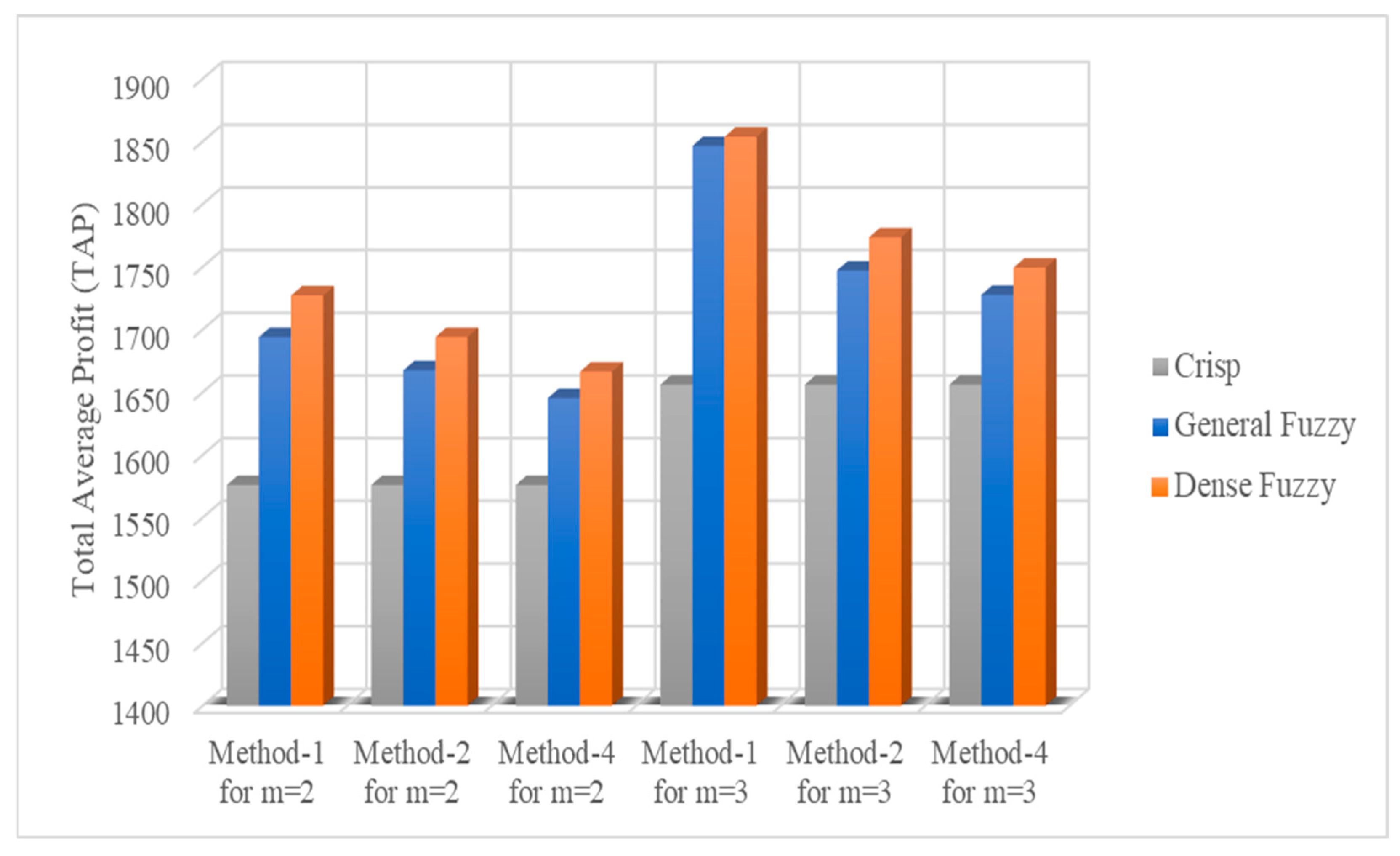
- As the repetition of the trial to fix the purchase cost–order quantity combination advances, the total average profit in the respective methods and fuzzy environments increase initially and again decrease for trials after . The best results for profit maximization goal are obtained for .
- The ordering of the best phenomena for maximizing average profit for every choice of is as follows:
- The dense fuzzy is perceived to be superior to the general fuzzy as decision-making phenomena to maximize the average profit irrespective of the methods and choices of .
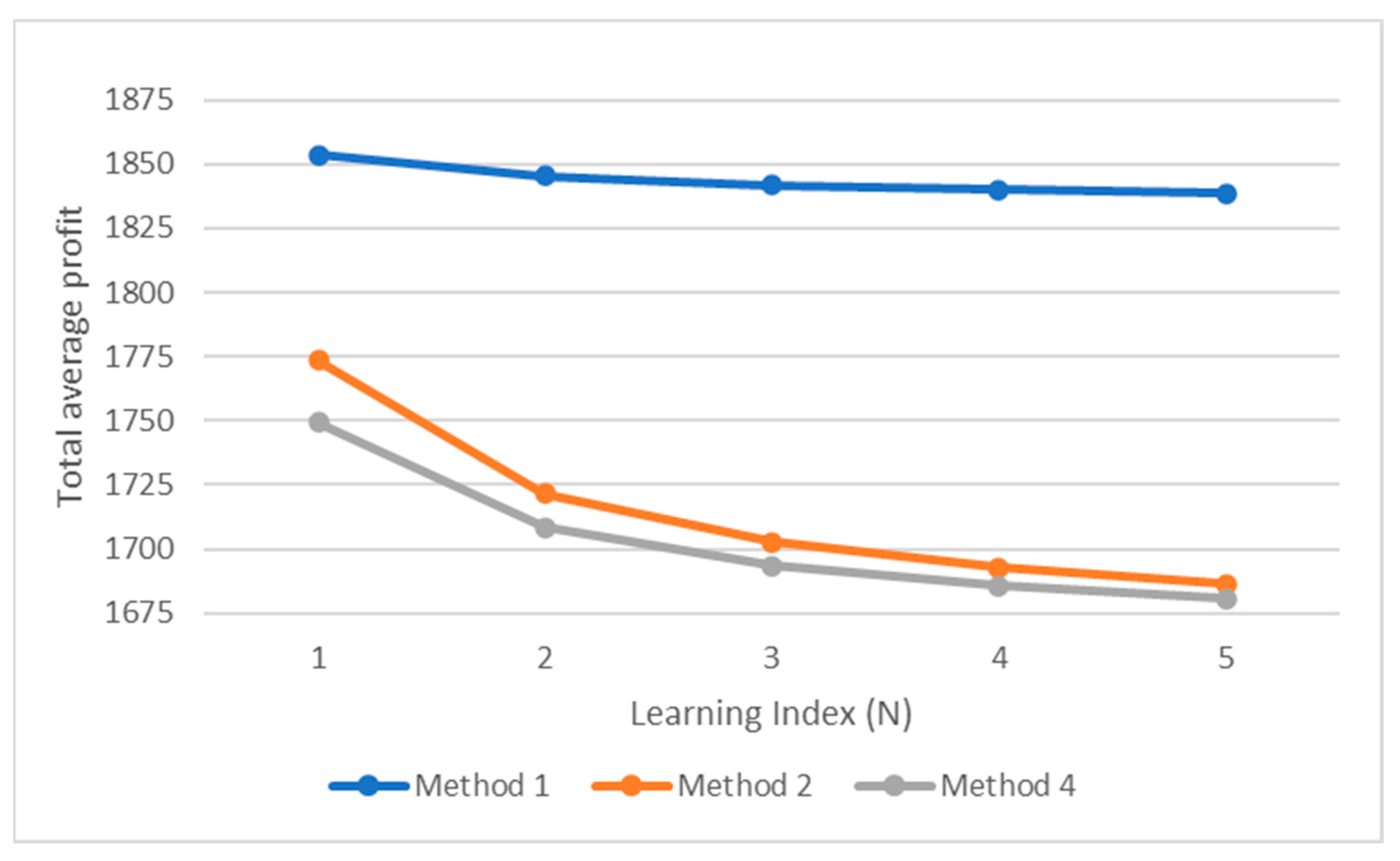
6.4. Learning Sensitivity in the Dense Fuzzy Environment
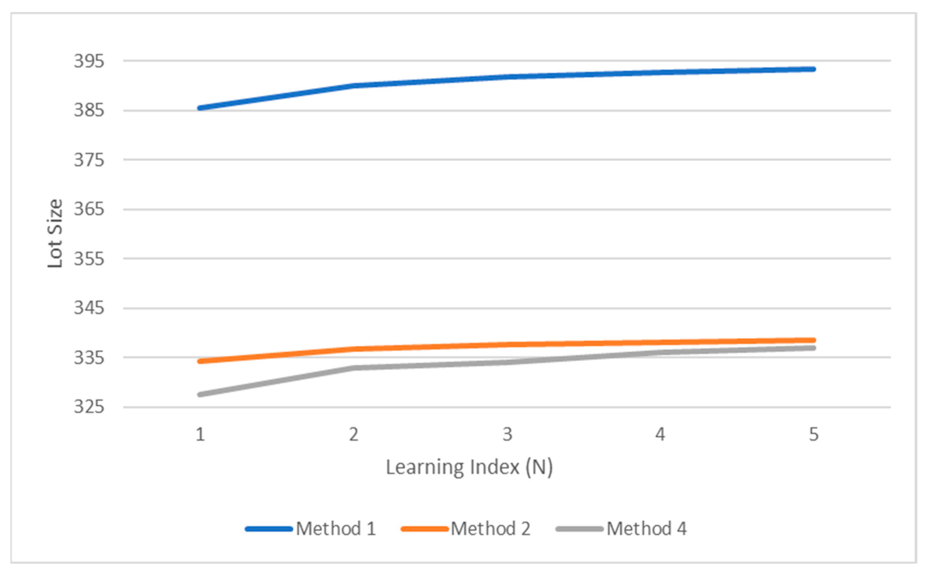
- The lot increases with the learning index when using each method. The largest lot size is obtained using method 1, while the smallest corresponds to method 4.
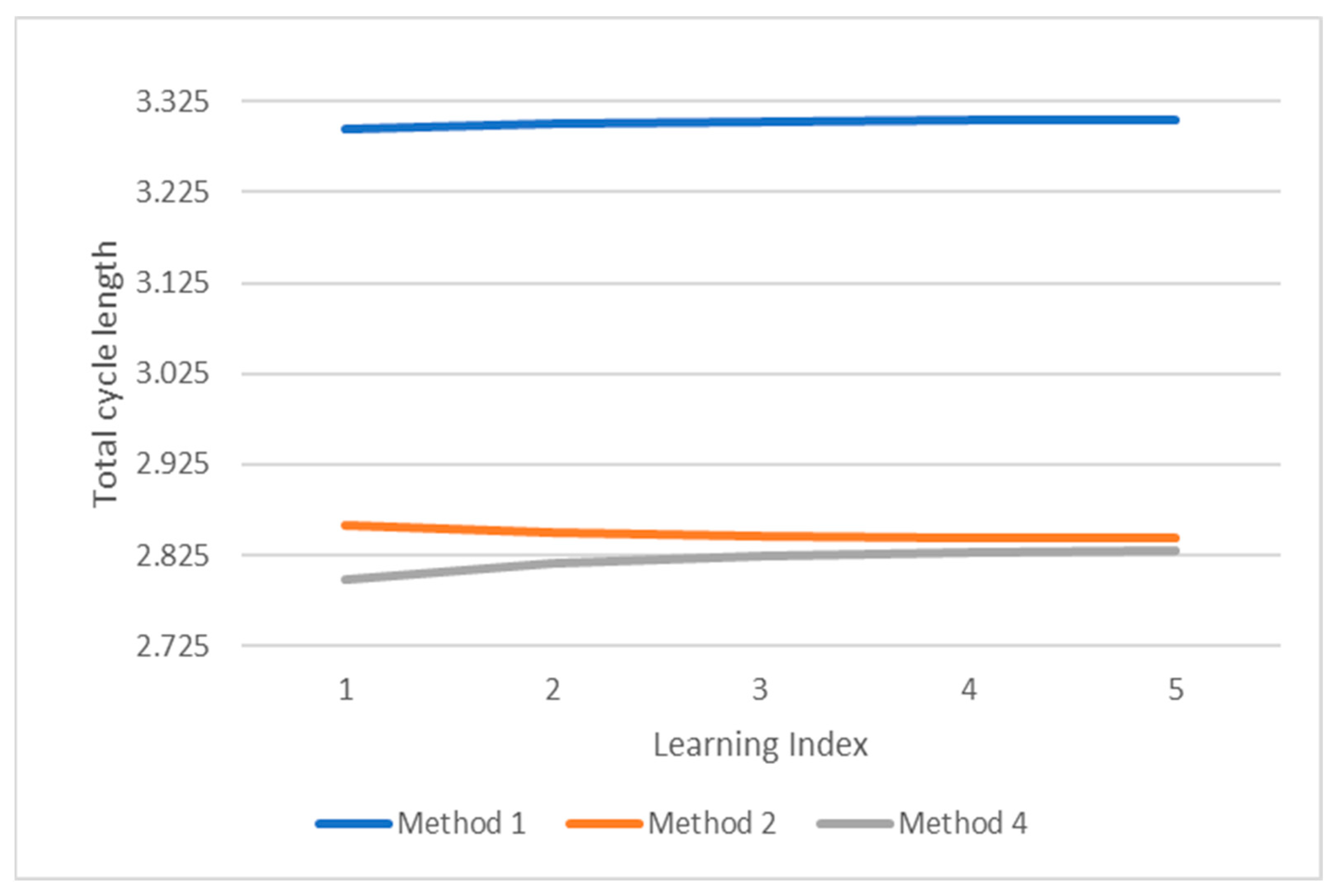
- The total cycle length increases with the learning index when using method 1 and method 4. The graph of the total cycle length shows the reverse pattern for method 2. The largest lot size is obtained using method 1, while the smallest corresponds to method 4.
- The total average profit decreases with the learning index when using each method. The best result corresponds to method 1.
7. Discussion on Numerical Results and Their Managerial Insights
- To design a strategy that should be used in an EOQ-driven marketing situation where consumers’ unpredictable demands rely on the unit selling price.
- To measure the impact of the unpredictable demand pattern on the decision-making process.
- To trace the sensitivity of the profit-maximizing policy on the all-unit price discount facility during purchasing.
- To address the question: how much can the decision-maker learn by doing repetitive tasks to implement a more effective plan and accomplish his/her goal?
- The purchase cost per unit is connected to lot size. It is observed that the lot size increases as the purchase cost per unit decrease. The decision-maker can be successfully persuaded to place larger orders using the planned all-unit discount policy on the purchase price per unit. As a result, the decision-maker should select the supplier that permits a plan for all-unit discounts on the purchase price. A trial to fix the purchase cost–order quantity combination using repetition is necessary for the feasible optimal solution. Feasibility does not occur before a specific trial. The decision-maker must first complete trial-and-error tasks to obtain a viable solution.
- After obtaining feasible solutions, the decision-makers will find the best one favoring their goal. As the number of trials increases, the average profit increases initially and, after reaching a peak, it then decreases. So, there will be an optimal choice for the trial number for profit maximization.
- The demand pattern of an item is not at all predictable, and uncertainties are involved with it. Fuzzy decision-making techniques are preferable to predict the demand pattern as well. The decision-makers must self-learn by performing repetitive tasks in a specific retailing cycle to pursue precision in the optimal retailing policy. Because the tasks are repeated frequently, the decision-maker can more precisely understand the demand rate. Thus, the dense fuzzy phenomenon is superior to the general fuzzy phenomenon for the profit maximization objective.
- However, the total cycle length and lot size increase with the learning index. That is, too much repetition causes the decision cycle to be unnecessarily large, which results in a deduction in the average profit. So, learning through repetition is necessary, but uncontrolled exercises may cause a backlash.
8. Conclusions and Future Research Scopes
Author Contributions
Funding
Data Availability Statement
Acknowledgments
Conflicts of Interest
Appendix A
References
- Harris, F.W. How many parts to make at once. Fact.-Mag. Manag. 1913, 10, 135–136. [Google Scholar] [CrossRef]
- Hadley, G.; Whitin, T.M. Analysis of Inventory Systems; Prentice-Hall: Englewood Cliffs, NJ, USA, 1963. [Google Scholar]
- Naddor, E. Inventory Systems; John Wiley: New York, NY, USA, 1966. [Google Scholar]
- Silver, E.A.; Meal, H.C. A heuristic for selecting lot size quantities for the case of a deterministic time varying demand rate and discrete opportunities for replenishment. Prod. Inventory Manag. 1973, 14, 64–74. [Google Scholar]
- Giri, B.C.; Pal, S.; Goswami, A.; Chaudhuri, K.S. An inventory model for deteriorating items with stock-dependent demand rate. Eur. J. Oper. Res. 1996, 95, 604–610. [Google Scholar] [CrossRef]
- Kim, J.; Hwang, H.; Shinn, S. An optimal credit policy to increase supplier’s profits with price-dependent demand functions. Prod. Plan. Control 1995, 6, 45–50. [Google Scholar] [CrossRef]
- Roy, A. An inventory model for deteriorating items with price dependent demand and time varying holding cost. Adv. Model. Optim. 2008, 10, 25–37. [Google Scholar]
- Tripathy, C.K.; Mishra, U. An inventory model for Weibull deteriorating items with price dependent demand and time-varying holding cost. Appl. Math. Sci. 2010, 4, 2171–2179. [Google Scholar]
- Alfares, H.K.; Ghaithan, A.M. EOQ and EPQ production inventory models with variable holding cost: State-of-the-art review. Arab. J. Sci. Eng. 2019, 44, 1737–1755. [Google Scholar] [CrossRef]
- Bhunia, A.; Shaikh, A. A deterministic inventory model for deteriorating items with selling price dependent demand and three-parameter Weibull distributed deterioration. Int. J. Ind. Eng. Comput. 2014, 5, 497–510. [Google Scholar] [CrossRef]
- Pal, S.; Mahapatra, G.S.; Samanta, G.P. An inventory model of price and stock dependent demand rate with deterioration under inflation and delay in payment. Int. J. Syst. Assur. Eng. Manag. 2014, 5, 591–601. [Google Scholar] [CrossRef]
- Ghoreishi, M.; Weber, G.W.; Mirzazadeh, A. An inventory model for non-instantaneous deteriorating items with partial backlogging, permissible delay in payments, inflation- and selling price-dependent demand and customer returns. Ann. Oper. Res. 2015, 226, 221–238. [Google Scholar] [CrossRef]
- Taleizadeh, A.A.; Noori-Daryan, M.; Govindan, K. Pricing and ordering decisions of two competing supply chains with different composite policies: A Stackelberg game-theoretic approach. Int. J. Prod. Res. 2016, 54, 2807–2836. [Google Scholar] [CrossRef]
- Mishra, U.; Barron, L.E.C.; Tiwari, S.; Shaikh, A.A.; Graza, G.T. An inventory model under price and stock dependent demand for controllable deterioration rate with shortages and preservation technology investment. Ann. Oper. Res. 2017, 254, 165–190. [Google Scholar] [CrossRef]
- Panda, G.C.; Khan, M.A.A.; Shaikh, A.A. A credit policy approach in a two-warehouse inventory model for deteriorating items with price- and stock-dependent demand under partial backlogging. J. Ind. Eng. Int. 2019, 15, 147–170. [Google Scholar] [CrossRef]
- Barron, L.E.C.; Shaikh, A.A.; Tiwari, S.; Garza, G.T. An EOQ inventory model with nonlinear stock dependent holding cost, nonlinear stock dependent demand and trade credit. Comput. Ind. Eng. 2020, 139, 105557. [Google Scholar] [CrossRef]
- Alfares, H.K.; Ghaithan, A.M. A Generalized Production-Inventory Model with Variable Production, Demand, and Cost Rates. Arab. J. Sci. Eng. 2022, 47, 3963–3978. [Google Scholar] [CrossRef]
- Akhtar, M.; Duary, A.; Manna, A.K.; Shaikh, A.A.; Bhunia, A.K. An application of tournament differential evolution algorithm in production inventory model with green level and expiry time dependent demand. Artif. Intell. Rev. 2022, 56, 4137–4170. [Google Scholar] [CrossRef]
- Hakim, M.A.; Hezam, I.M.; Alrasheedi, A.F.; Gwak, J. Pricing Policy in an Inventory Model with Green Level Dependent Demand for a Deteriorating Item. Sustainability 2022, 14, 4646. [Google Scholar] [CrossRef]
- Shi, J.; Zhang, G.; Lai, K.K. Optimal ordering and pricing policy with supplier quantity discounts and price-dependent stochastic demand. Optimization 2012, 61, 151–162. [Google Scholar] [CrossRef]
- Chen, S.P.; Ho, Y.H. Optimal inventory policy for the fuzzy newsboy problem with quantity discounts. Inf. Sci. 2013, 228, 75–89. [Google Scholar] [CrossRef]
- Taleizadeh, A.A.; Pentico, D.W. An economic order quantity model with partial backordering and all-units discount. Int. J. Prod. Econ. 2014, 155, 172–184. [Google Scholar] [CrossRef]
- Taleizadeh, A.A.; Stojkovska, I.; Pentico, D.W. An economic order quantity model with partial backordering and incremental discount. Comput. Ind. Eng. 2015, 82, 21–32. [Google Scholar] [CrossRef]
- Alfares, H.K. Maximum-profit inventory model with stock-dependent demand, time dependent holding cost, and all-units quantity discounts. Math. Model. Anal. 2015, 20, 715–736. [Google Scholar] [CrossRef]
- Alfares, H.K.; Ghaithan, A.M. Inventory and pricing model with price-dependent demand, time-varying holding cost, and quantity discounts. Comput. Ind. Eng. 2016, 94, 170–177. [Google Scholar] [CrossRef]
- Huang, T.S.; Yang, M.F.; Chao, Y.S.; Kei, E.S.Y.; Chung, W.H. Fuzzy Supply Chain Integrated Inventory Model with Quantity Discounts and Unreliable Process in Uncertain Environments. In Proceedings of the International MultiConference of Engineers and Computer Scientists, Hong Kong, China, 14–16 March 2018; Volume 2, pp. 14–16. [Google Scholar]
- Sebatjane, M.; Adetunji, O. Economic order quantity model for growing items with incremental quantity discounts. J. Ind. Eng. Int. 2019, 15, 545–556. [Google Scholar] [CrossRef]
- Shaikh, A.A.; Khan, M.A.A.; Panda, G.C.; Konstantaras, I. Price discount facility in an EOQ model for deteriorating items with stock-dependent demand and partial backlogging. Int. Trans. Oper. Res. 2019, 26, 1365–1395. [Google Scholar] [CrossRef]
- Khan, M.A.A.; Ahmed, S.; Babu, M.S.; Sultana, N. Optimal lot-size decision for deteriorating items with price-sensitive demand, linearly time-dependent holding cost under all-units discount environment. Int. J. Syst. Sci. Oper. Logist. 2020, 9, 61–74. [Google Scholar] [CrossRef]
- Mashud, A.H.M.; Roy, D.; Daryanto, Y.; Wee, H.M. Joint pricing deteriorating inventory model considering product life cycle and advance payment with a discount facility. RAIRO-Oper. Res. 2021, 55, S1069–S1088. [Google Scholar] [CrossRef]
- Rahman, M.S.; Duary, A.; Khan, M.A.A.; Shaikh, A.A.; Bhunia, A.K. Interval valued demand related inventory model under all-units discount facility and deterioration via parametric approach. Artif. Intell. Rev. 2022, 55, 2455–2494. [Google Scholar] [CrossRef]
- Kuppulakshmi, V.; Sugapriya, C.; Kavikumar, J.; Nagarajan, D. Fuzzy Inventory Model for Imperfect Items with Price Discount and Penalty Maintenance Cost. Math. Probl. Eng. 2023, 2023, 1246257. [Google Scholar] [CrossRef]
- Zadeh, L.A. Fuzzy sets. Inf. Control 1965, 8, 338–353. [Google Scholar] [CrossRef]
- Kaleva, O. Fuzzy differential equations. Fuzzy Sets Syst. 1987, 24, 301–317. [Google Scholar] [CrossRef]
- Park, K.S. Fuzzy-set theoretic interpretation of economic order quantity. IEEE Trans. Syst. Man Cybern. 1987, 17, 1082–1084. [Google Scholar] [CrossRef]
- Debnath, B.K.; Majumder, P.; Bera, U.K.; Maiti, M. Inventory model with demand as type-2 fuzzy number: A fuzzy differential equation approach. Iran. J. Fuzzy Syst. 2018, 15, 1–24. [Google Scholar]
- Guchhait, P.; Maiti, M.K.; Maiti, M. A production inventory model with fuzzy production and demand using fuzzy differential equation: An interval compared genetic algorithm approach. Eng. Appl. Artif. Intell. 2013, 26, 766–778. [Google Scholar] [CrossRef]
- Mahata, G.C.; De, S.K.; Bhattacharya, K.; Maity, S. Three-echelon supply chain model in an imperfect production system with inspection error, learning effect, and return policy under fuzzy environment. Int. J. Syst. Sci. Oper. Logist. 2021, 10, 1962427. [Google Scholar] [CrossRef]
- Manna, A.K.; Barron, L.E.C.; Dey, J.K.; Mondal, S.K.; Shaikh, A.A.; Mota, A.C.; Garza, G.T. A fuzzy imperfect production inventory model based on fuzzy differential and fuzzy integral method. J. Risk Financ. Manag. 2022, 15, 239. [Google Scholar] [CrossRef]
- Wright, T.P. Factors affecting the cost of airplanes. J. Aeronaut. Sci. 1936, 3, 122–128. [Google Scholar] [CrossRef]
- Glock, C.H.; Schwindl, K.; Jaber, M.Y. An EOQ model with fuzzy demand and learning in fuzziness. Int. J. Serv. Oper. Manag. 2012, 12, 90–100. [Google Scholar] [CrossRef]
- Mahata, G.C. A production-inventory model with imperfect production process and partial backlogging under learning considerations in fuzzy random environments. J. Intell. Manuf. 2014, 28, 883–897. [Google Scholar] [CrossRef]
- Kumar, R.S.; Goswami, A. EPQ model with learning consideration, imperfect production and partial backlogging in fuzzy random environment. Int. J. Syst. Sci. 2015, 46, 1486–1497. [Google Scholar] [CrossRef]
- Kazemi, N.; Shekarian, E.; Barron, L.E.C. Incorporating human learning into a fuzzy EOQ inventory model with backorders. Comput. Ind. Eng. 2015, 87, 540–542. [Google Scholar] [CrossRef]
- Shekarian, E.; Olugu, E.U.; Rashid, S.H.A.; Kazemi, N. An economic order quantity model considering different holding costs for imperfect quality items subject to fuzziness and learning. J. Intell. Fuzzy Syst. 2016, 30, 2985–2997. [Google Scholar] [CrossRef]
- Kazemi, N.; Rashid, S.H.A.; Shekarian, E.; Bottani, E.; Montanari, R. A fuzzy lot-sizing problem with two stage composite human learning. Int. J. Prod. Res. 2016, 54, 5010–5025. [Google Scholar] [CrossRef]
- Soni, H.N.; Sarkar, B.; Joshi, M. Demand uncertainty and learning in fuzziness in a continuous review inventory model. J. Intell. Fuzzy Syst. 2017, 33, 2595–2608. [Google Scholar] [CrossRef]
- De, S.K.; Beg, I. Triangular dense fuzzy sets and new defuzzification methods. J. Intell. Fuzzy Syst. 2016, 31, 469–477. [Google Scholar] [CrossRef]
- De, S.K. Triangular dense fuzzy lock sets. Soft Comput. 2018, 22, 7243–7254. [Google Scholar] [CrossRef]
- Maity, S.; De, S.K.; Mondal, S.P. A Study of an EOQ Model under Lock Fuzzy Environment. Mathematics 2019, 7, 75. [Google Scholar] [CrossRef]
- Rahaman, M.; Mondal, S.P.; Alam, S. An estimation of effects of memory and learning experience on the EOQ model with price dependent demand. RAIRO-Oper. Res. 2021, 55, 2991–3020. [Google Scholar] [CrossRef]
- Rahaman, M.; Mondal, S.P.; Alam, S.; Goswami, A. Synergetic study of inventory management problem in uncertain environment based on memory and learning effects. Sadhana 2021, 46, 39. [Google Scholar] [CrossRef]
- Yager, R.R. A procedure for ordering fuzzy subsets of the unit interval. Inf. Sci. 1981, 24, 143–161. [Google Scholar] [CrossRef]


| References | Year | Model Type | Model Features | Discount Type | Discount Environment |
|---|---|---|---|---|---|
| Shi et al. [20] | 2012 | NP | Price-dependent demand and supplier quantity discount | All-unit quantity discount | Crisp |
| Chen and Ho [21] | 2013 | NP | Fuzzy constant demand and quantity discount | All-unit quantity discount | Crisp |
| Taleizadeh and Pentico [22] | 2014 | EOQ | Constant demand, partial backordering, and supplier quantity discount | All-unit quantity discount | Crisp |
| Taleizadeh et al. [23] | 2015 | EOQ | Constant demand, discount facility, and partial backordering | Incremental discount | Crisp |
| Alfares [24] | 2015 | EPQ | Stock dependent demand, discount policy, and variable holding cost | All-unit quantity discount | Crisp |
| Alfares and Ghaithan [25] | 2016 | EOQ | Price-dependent demand, time varying holding cost, and quantity discount | All-unit quantity discount | Crisp |
| Huang et al. [26] | 2018 | EPQ | Fuzzy constant demand, unreliable process, and quantity discount | Fixed discount rate | Fuzzy |
| Sebatjane and Adetunji [27] | 2019 | EOQ | Constant demand and growing items | Incremental quantity discount | Crisp |
| Shaikh et al. [28] | 2019 | EOQ | Stock dependent demand, constant deterioration, partially backlogging shortage, and holding cost proportional to purchase cost and time varying | All-unit quantity discount | Crisp |
| Khan et al. [29] | 2020 | EOQ | Price dependent demand, constant deterioration, and holding cost proportional to purchase cost and time varying | All-unit quantity discount | Crisp |
| Mashud et al. [30] | 2021 | EOQ | Price dependent demand, advance payment, time varying deterioration, and time varying holding cost | All-unit quantity discount | Crisp |
| Rahman et al. [31] | 2022 | EOQ | Stock dependent demand, deteriorating items, and with and without shortage | All-unit quantity discount | Interval |
| Kuppulakshmi et al. [32] | 2023 | EPQ | Fuzzy demand and imperfect product | Price discount | Fuzzy |
| References | Year | Model Description | Applied Learning Concept on | Learning Method | Application Area |
|---|---|---|---|---|---|
| Glock et al. [41] | 2012 | EOQ model with fuzzy demand | Customer demand | Wright’s power function formula | Firm practitioners |
| Mahata [42] | 2014 | Inventory model for an imperfect product considering partial backlogging in a fuzzy environment based on the credibility measure of a fuzzy event | Production time | Wright’s power function formula | General application in production inventory |
| Kumar et al. [43] | 2015 | EPQ model with partial backlogging and process shifting | Production time | Wright’s power function formula | Decorative manufactures company |
| Kazemi et al. [44] | 2015 | Backorder EOQ model with learning rate under a fuzzy environment | Order quantity | Wright’s power function formula | Paper distribution problem |
| Shekarian et al. [45] | 2016 | EOQ model of imperfect product with constant demand under fuzziness | Defective items | S-shaped logistic curve model | General manufacturing problem |
| Kazemi et al. [46] | 2016 | Backorder fuzzy EOQ model with two-level combined human learning | Demand, maximum inventory level | Jaber–Glock learning curve model | Paper distribution problem |
| Soni et al. [47] | 2017 | Continuous review inventory system with shortage and triangular fuzzy demand | Demand function, ordering quantity | Wright’s power function formula | General ordering application |
| Maity et al. [50] | 2019 | EOQ model under daytime with uncertain demand | Holding cost, demand rate, set up cost, idle time cost | Triangular dense fuzzy lock set | Newly open shop/industry |
| Rahaman et al. [51] | 2021 | EOQ model with price-sensitive demand considering the effect of memory and experience-based learning | Unit selling price, demand rate | Triangular dense fuzzy lock set | General ordering problem |
| Rahaman et al. [52] | 2021 | Memory and learning effecting inventory management problem | Demand rate | Triangular dense fuzzy set | General ordering problem |
| Notations | Description |
|---|---|
| Fixed part of the demand function | |
| Coefficient of the price in the demand function | |
| Unit selling price (decision variable) ($/unit) | |
| Triangular dense fuzzy valued unit selling price (decision variable) ($/unit) | |
| Fixed part of the per unit holding cost ( | |
| Coefficient of time in the per unit holding cost ( | |
| Number of repetitions that dilute fuzzy impreciseness in the dense fuzzy variable (non-negative integer) | |
| Function of the per unit purchasing cost (decision variable) ($/unit) | |
| Per unit crisp purchasing cost (decision variable) ($/unit) | |
| Number of repetitions for adjusting and scaling (non-negative integer) for a given lot size | |
| Scaling parameter in ( | |
| Triangular dense fuzzy valued unit purchasing cost (decision variable) ($/unit) | |
| Quantities that determine the price breaks in the discount environment | |
| Triangular dense fuzzy valued quantities that determine the price breaks in the discount environment | |
| Deviation indicator of the triangular dense fuzzy-valued unit price | |
| Deviation indicator of triangular dense fuzzy-valued unit purchasing cost | |
| Deviation indicator of triangular dense fuzzy-valued quantities that determines the price breaks | |
| Demand function (unit/cycle) | |
| Per cycle ordering cost ($/cycle) | |
| Level of stock at any time | |
| Ordering size (decision variable) (unit/cycle) | |
| Total cycle length (decision variable) (months) | |
| Total average profit (objective function) ($/cycle) | |
| Index value, i.e., the defuzzified value of the |
| Repeat () | 0 | 1 | 2 | 3 | 4 | 5 |
|---|---|---|---|---|---|---|
| Order quantity size | [0, 100] | [100, 200] | [200, 300] | [300, 400] | [400, 500] | [500, 600] |
| Purchasing cost per unit | 5.00 | 4.50 | 4.00 | 3.50 | 3.00 | 2.50 |
| Repeat (m) | Observation | |||||
|---|---|---|---|---|---|---|
| 0 | 5.00 | 20 | 292.17 | 2.435 | 1418.91 | Q is not matched |
| 1 | 4.50 | 20 | 305.90 | 2.549 | 1496.96 | Q is not matched |
| 2 | 4.00 | 20 | 321.95 | 2.683 | 1576.06 | Q is not matched |
| 3 | 3.50 | 20 | 341.06 | 2.842 | 1656.43 | Q is matched |
| 4 | 3.00 | 20 | 364.41 | 3.037 | 1738.36 | Q is not matched |
| 5 | 2.50 | 20 | 393.87 | 3.282 | 1822.26 | Q is not matched |
| Repeat (m) | Method | Repeat () | Observation | ||||||
|---|---|---|---|---|---|---|---|---|---|
| 0 | Crisp | [0, 100] | 5.00 | 20 | 292.17 | 2.435 | 1418.92 | is not matched | |
| Method 1 | General Fuzzy | [0, 105] | 5.125 | 20.5 | 286.31 | 2.426 | 1431.78 | is not matched | |
| Dense fuzzy (n = 1) | [0, 107.5] | 5.188 | 20.25 | 283.44 | 2.422 | 1437.71 | is not matched | ||
| Method 2 | General Fuzzy | [0, 105] | 5.125 | 20.5 | 288.77 | 2.447 | 1511.97 | is not matched | |
| Dense fuzzy (n = 1) | [0, 107.5] | 5.188 | 20.25 | 286.43 | 2.448 | 1538.62 | is not matched | ||
| Method 4 | General Fuzzy | [0, 105] | 5.125 | 20.5 | 283.94 | 2.406 | 1484.50 | is not matched | |
| Dense fuzzy (n = 1) | [0, 107.5] | 5.188 | 20.25 | 280.48 | 2.397 | 1504.30 | is not matched | ||
| 1 | Crisp | [100, 200] | 4.500 | 20 | 305.90 | 2.549 | 1496.96 | is not matched | |
| Method 1 | General Fuzzy | [105, 210] | 4.613 | 20.5 | 313.81 | 2.659 | 1582.00 | is not matched | |
| Dense fuzzy (n = 1) | [107.5, 215] | 4.669 | 20.25 | 310.66 | 2.655 | 1588.40 | is not matched | ||
| Method 2 | General Fuzzy | [105, 210] | 4.613 | 20.5 | 302.34 | 2.562 | 1589.21 | is not matched | |
| Dense fuzzy (n = 1) | [107.5, 215] | 4.669 | 20.25 | 299.89 | 2.563 | 1615.80 | is not matched | ||
| Method 4 | General Fuzzy | [105, 210] | 4.613 | 20.5 | 297.31 | 2.519 | 1564.42 | is not matched | |
| Dense fuzzy (n = 1) | [107.5, 215] | 4.669 | 20.25 | 293.68 | 2.510 | 1584.82 | is not matched | ||
| 2 | Crisp | [200, 300] | 4.000 | 20 | 321.95 | 2.683 | 1576.06 | is not matched | |
| Method 1 | General Fuzzy | [210, 315] | 4.100 | 20.5 | 347.38 | 2.944 | 1720.22 | is not matched | |
| Dense fuzzy (n = 1) | [215, 322.5] | 4.150 | 20.25 | 343.90 | 2.939 | 1727.06 | is not matched | ||
| Method 2 | General Fuzzy | [210, 315] | 4.100 | 20.5 | 318.20 | 2.696 | 1667.51 | is not matched | |
| Dense fuzzy (n = 1) | [215, 322.5] | 4.150 | 20.25 | 315.62 | 2.698 | 1694.04 | is matched | ||
| Method 4 | General Fuzzy | [210, 315] | 4.100 | 20.5 | 312.92 | 2.652 | 1645.40 | is matched | |
| Dense fuzzy (n = 1) | [215, 322.5] | 4.150 | 20.25 | 309.11 | 2.642 | 1666.42 | is matched | ||
| 3 | Crisp | [300, 400] | 3.500 | 20 | 341.06 | 2.842 | 1656.04 | is matched | |
| Method 1 | General Fuzzy | [315, 420] | 3.588 | 20.5 | 389.34 | 3.299 | 1846.48 | is matched | |
| Dense fuzzy (n = 1) | [322.5, 430] | 3.631 | 20.25 | 385.45 | 3.294 | 1853.71 | is matched | ||
| Method 2 | General Fuzzy | [315, 420] | 3.588 | 20.5 | 337.08 | 2.856 | 1747.06 | is matched | |
| Dense fuzzy (n = 1) | [322.5, 430] | 3.631 | 20.25 | 334.34 | 2.858 | 1773.54 | is matched | ||
| Method 4 | General Fuzzy | [315, 420] | 3.588 | 20.5 | 331.52 | 2.810 | 1727.68 | is matched | |
| Dense fuzzy (n = 1) | [322.5, 430] | 3.631 | 20.25 | 327.50 | 2.799 | 1749.32 | is matched |
| Method 1 | 1 | [322.50, 430.00] | 3.631 | 20.25 | 385.45 | 3.294 | 1853.70 |
| 2 | [313.75, 418.33] | 3.580 | 20.21 | 389.99 | 3.301 | 1845.23 | |
| 3 | [310.42, 413.89] | 3.561 | 20.18 | 391.74 | 3.303 | 1841.86 | |
| 4 | [308.56, 411.42] | 3.550 | 20.16 | 392.72 | 3.304 | 1839.94 | |
| 5 | [307.35, 409.80] | 3.543 | 20.14 | 393.36 | 3.305 | 1838.68 | |
| Method 2 | 1 | [322.50, 430.00] | 3.631 | 20.25 | 334.34 | 2.858 | 1773.54 |
| 2 | [313.75, 418.33] | 3.580 | 20.21 | 336.72 | 2.850 | 1721.72 | |
| 3 | [310.42, 413.89] | 3.561 | 20.18 | 337.66 | 2.847 | 1702.80 | |
| 4 | [308.56, 411.42] | 3.550 | 20.16 | 338.19 | 2.845 | 1692.72 | |
| 5 | [307.35, 409.80] | 3.543 | 20.14 | 338.55 | 2.844 | 1686.39 | |
| Method 4 | 1 | [322.50, 430.00] | 3.631 | 20.25 | 327.49 | 2.799 | 1749.32 |
| 2 | [313.75, 418.33] | 3.580 | 20.21 | 332.93 | 2.817 | 1708.52 | |
| 3 | [310.42, 413.89] | 3.561 | 20.18 | 334.10 | 2.824 | 1693.59 | |
| 4 | [308.56, 411.42] | 3.550 | 20.16 | 336.14 | 2.828 | 1685.62 | |
| 5 | [307.35, 409.80] | 3.543 | 20.14 | 336.87 | 2.830 | 1680.61 |
Disclaimer/Publisher’s Note: The statements, opinions and data contained in all publications are solely those of the individual author(s) and contributor(s) and not of MDPI and/or the editor(s). MDPI and/or the editor(s) disclaim responsibility for any injury to people or property resulting from any ideas, methods, instructions or products referred to in the content. |
© 2023 by the authors. Licensee MDPI, Basel, Switzerland. This article is an open access article distributed under the terms and conditions of the Creative Commons Attribution (CC BY) license (https://creativecommons.org/licenses/by/4.0/).
Share and Cite
Momena, A.F.; Rahaman, M.; Haque, R.; Alam, S.; Mondal, S.P. A Learning-Based Optimal Decision Scenario for an Inventory Problem under a Price Discount Policy. Systems 2023, 11, 235. https://doi.org/10.3390/systems11050235
Momena AF, Rahaman M, Haque R, Alam S, Mondal SP. A Learning-Based Optimal Decision Scenario for an Inventory Problem under a Price Discount Policy. Systems. 2023; 11(5):235. https://doi.org/10.3390/systems11050235
Chicago/Turabian StyleMomena, Alaa Fouad, Mostafijur Rahaman, Rakibul Haque, Shariful Alam, and Sankar Prasad Mondal. 2023. "A Learning-Based Optimal Decision Scenario for an Inventory Problem under a Price Discount Policy" Systems 11, no. 5: 235. https://doi.org/10.3390/systems11050235