
Optimizing Ultra-High Vacuum Control in Electron Storage Rings Using Fuzzy Control and Estimation of Pumping Speed by Neural Networks with Molflow+

Abstract
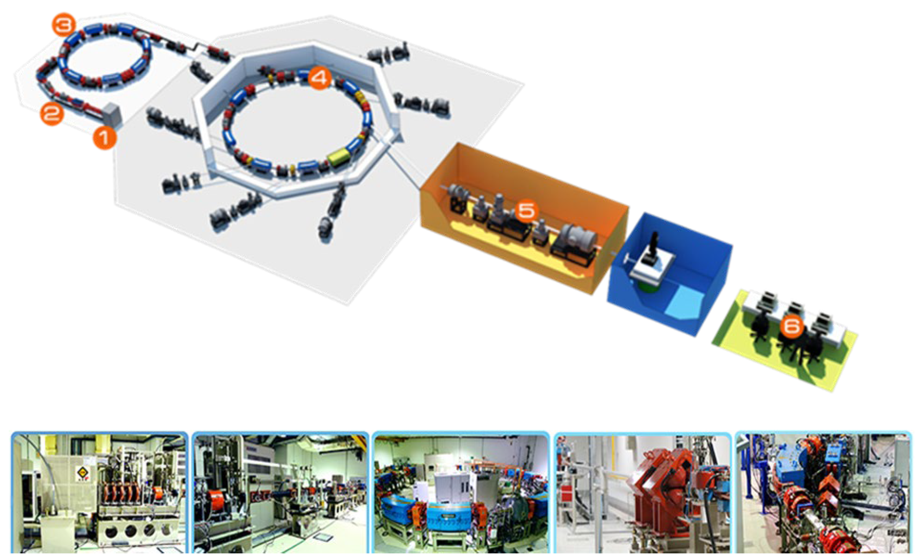
:1. Introduction
2. Materials and Methods
2.1. Research Methodology
2.2. Equipment
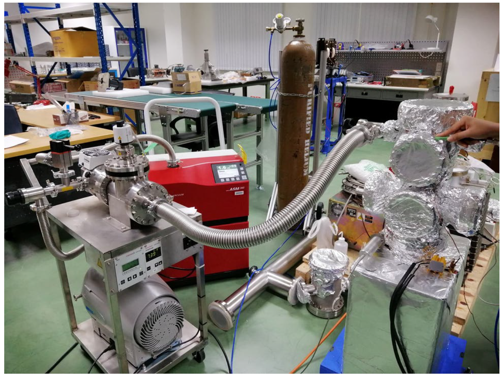
2.3. Experimental System
3. Ultra-High Vacuum by Fuzzy Control
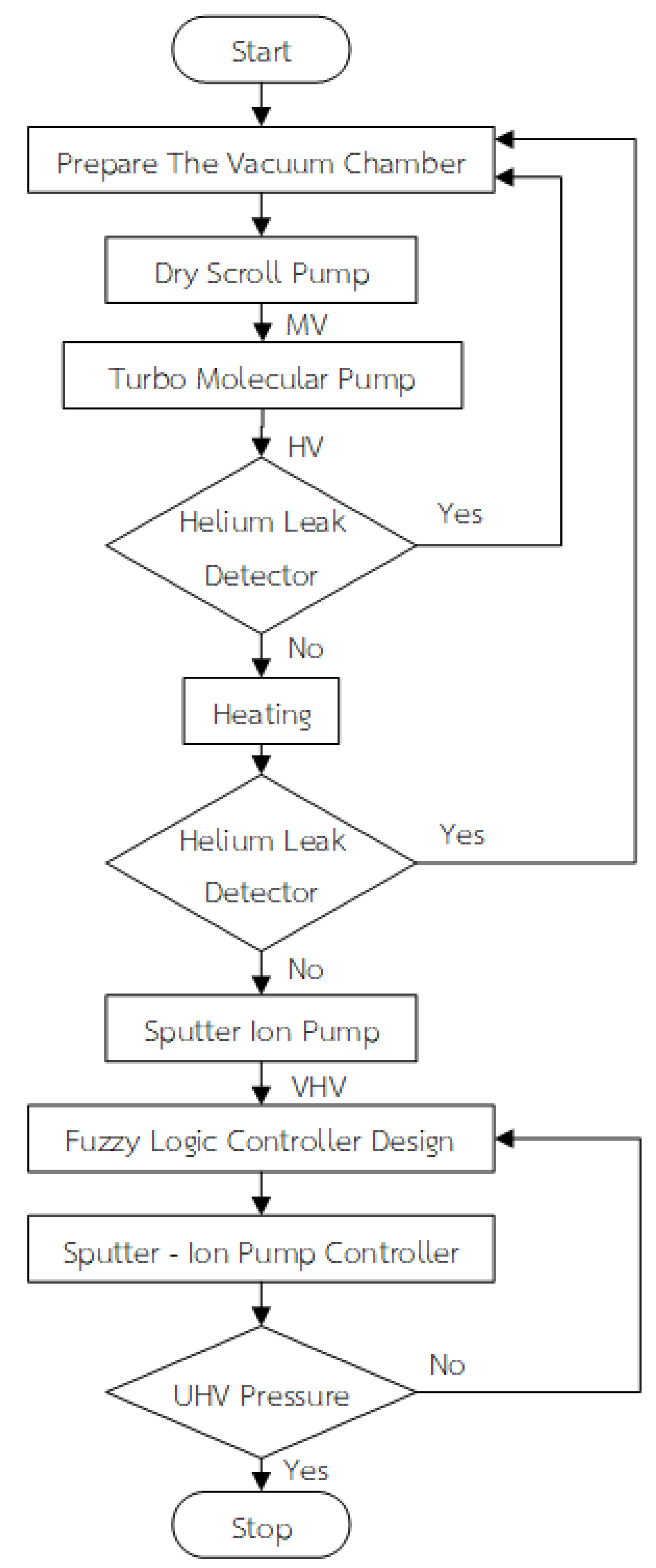
3.1. Procedure for Ultra-High Vacuum Pressure System
3.2. Procedure for Checking for Leaks in the Vacuum System
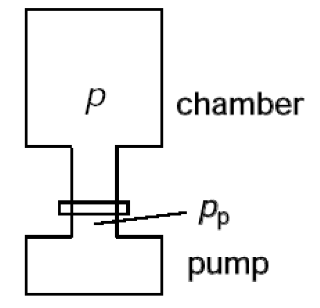
3.3. Sputter-Ion Pump
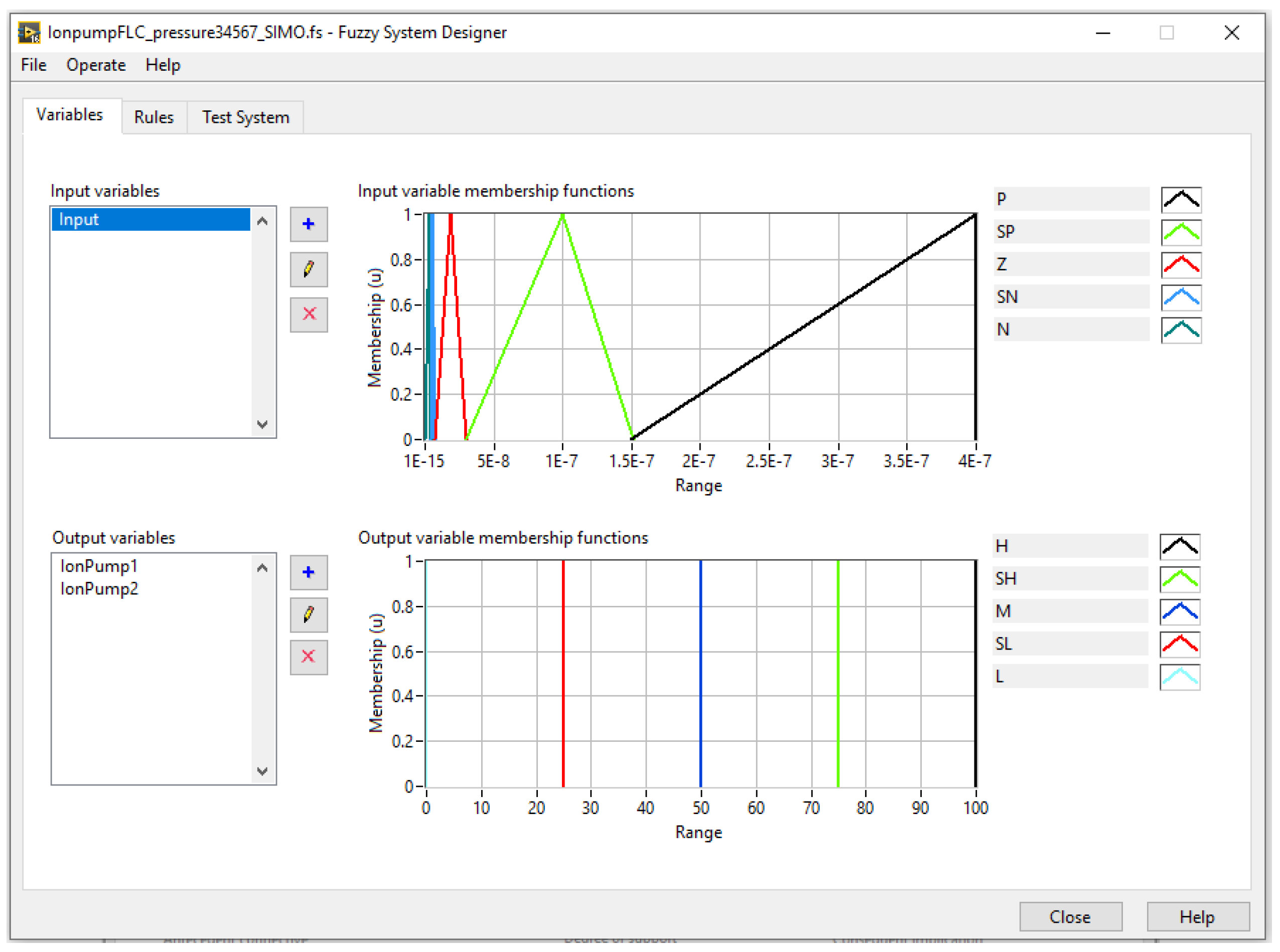
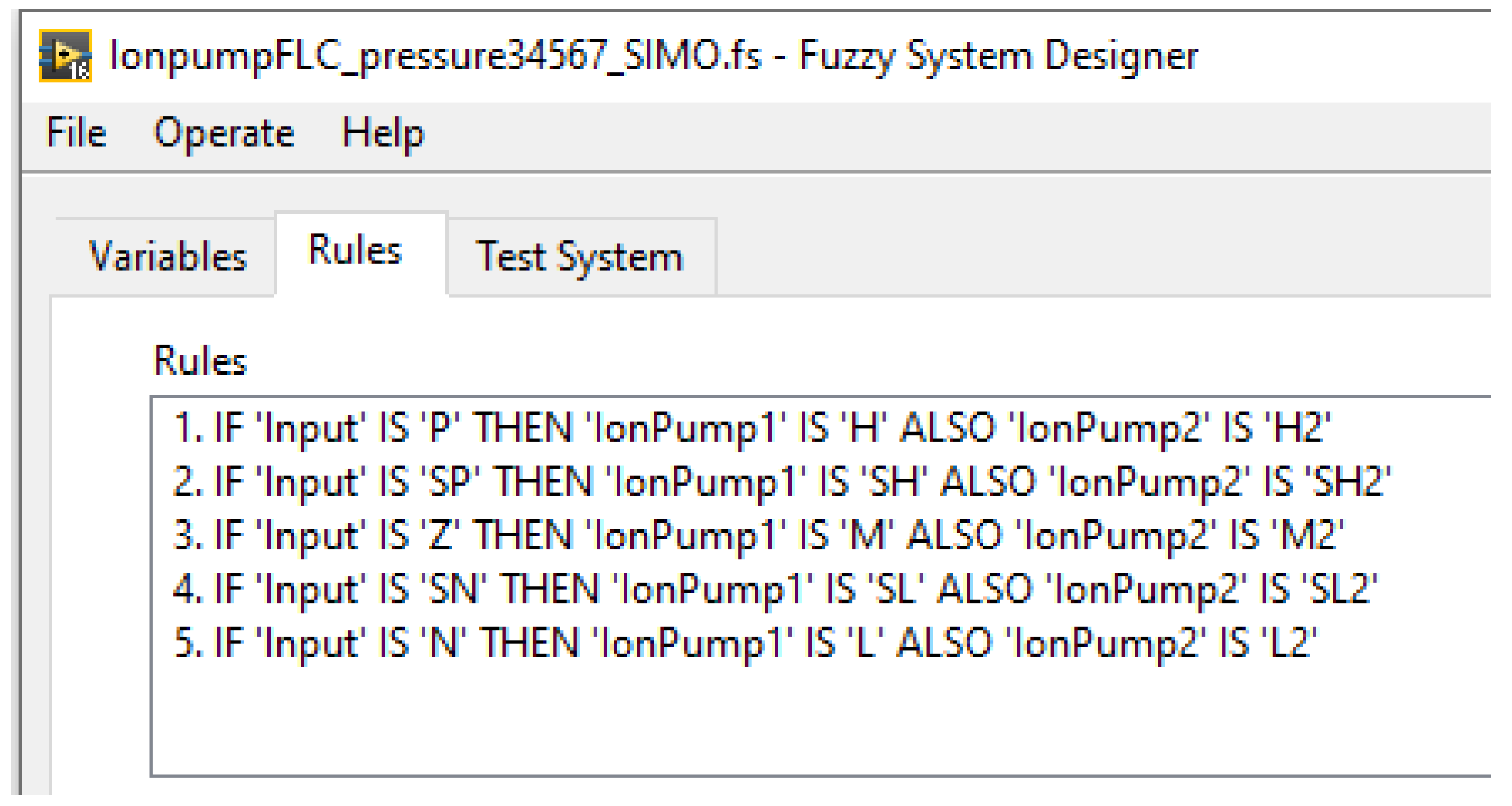
3.4. Fuzzy Design
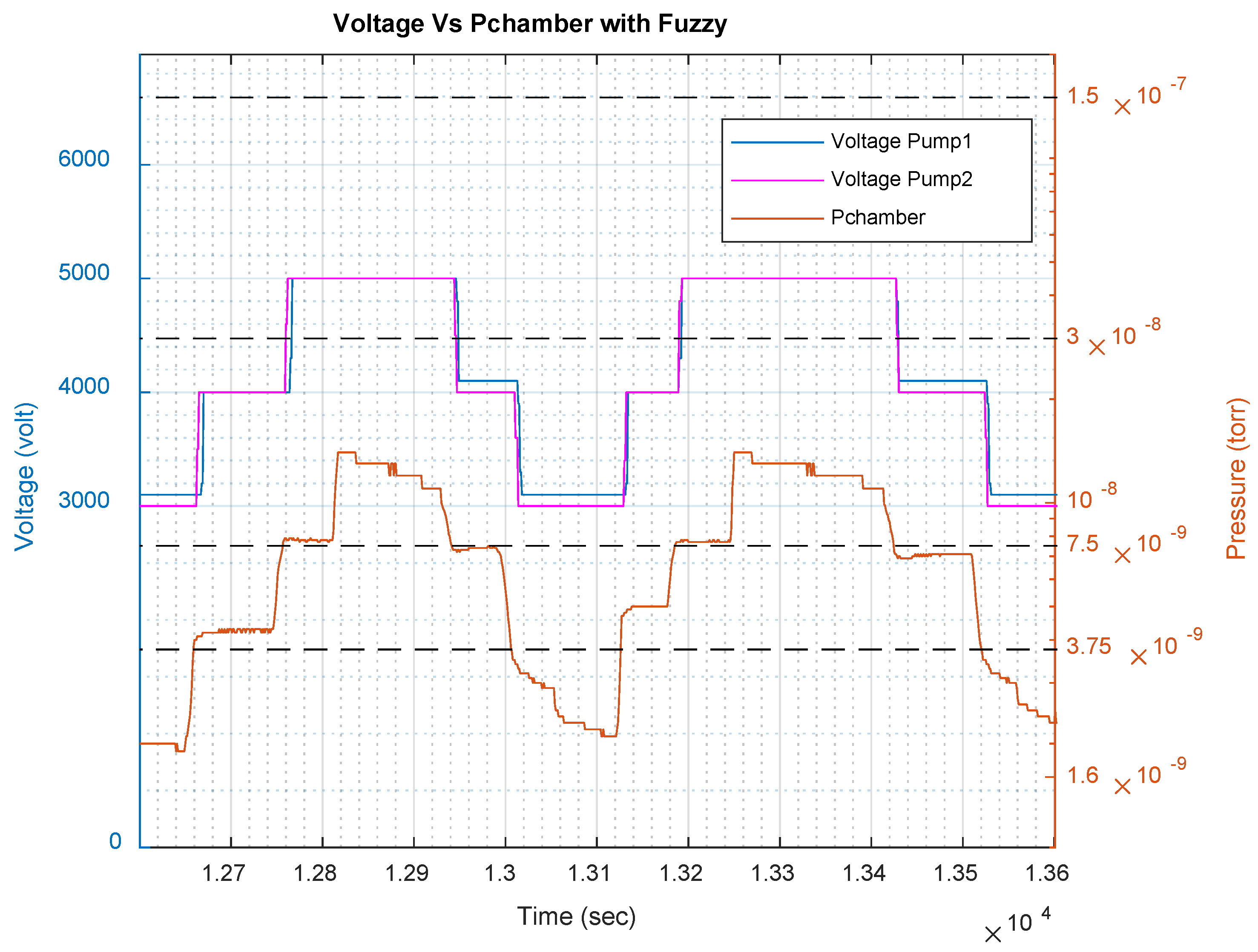
Fuzzy Pressure Control Improves Test System Performance
4. Pumping Speed Efficiency Estimation
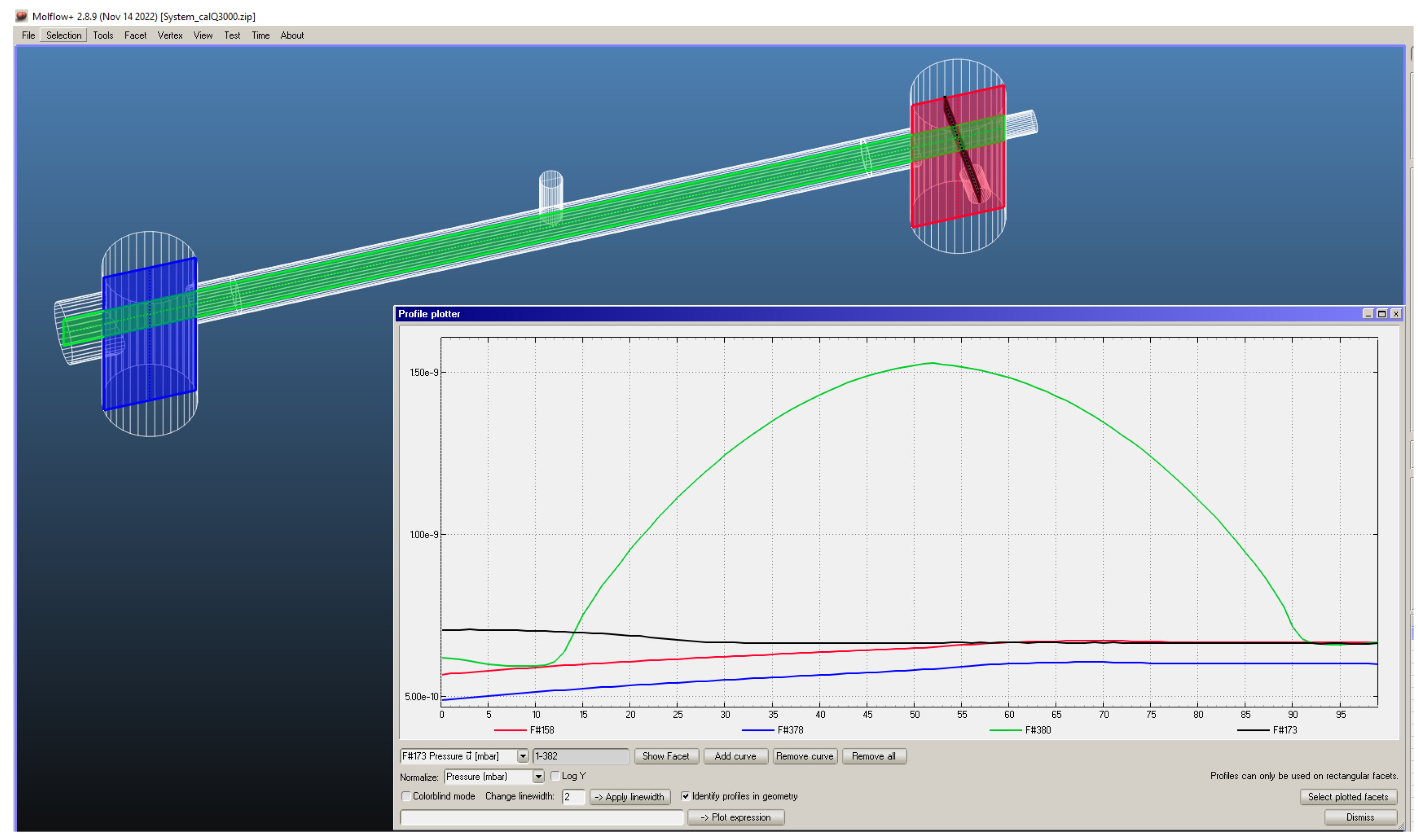
4.1. MolFlow+
4.2. Artificial Neural Network (ANN)
4.2.1. Data Collection and Preprocessing
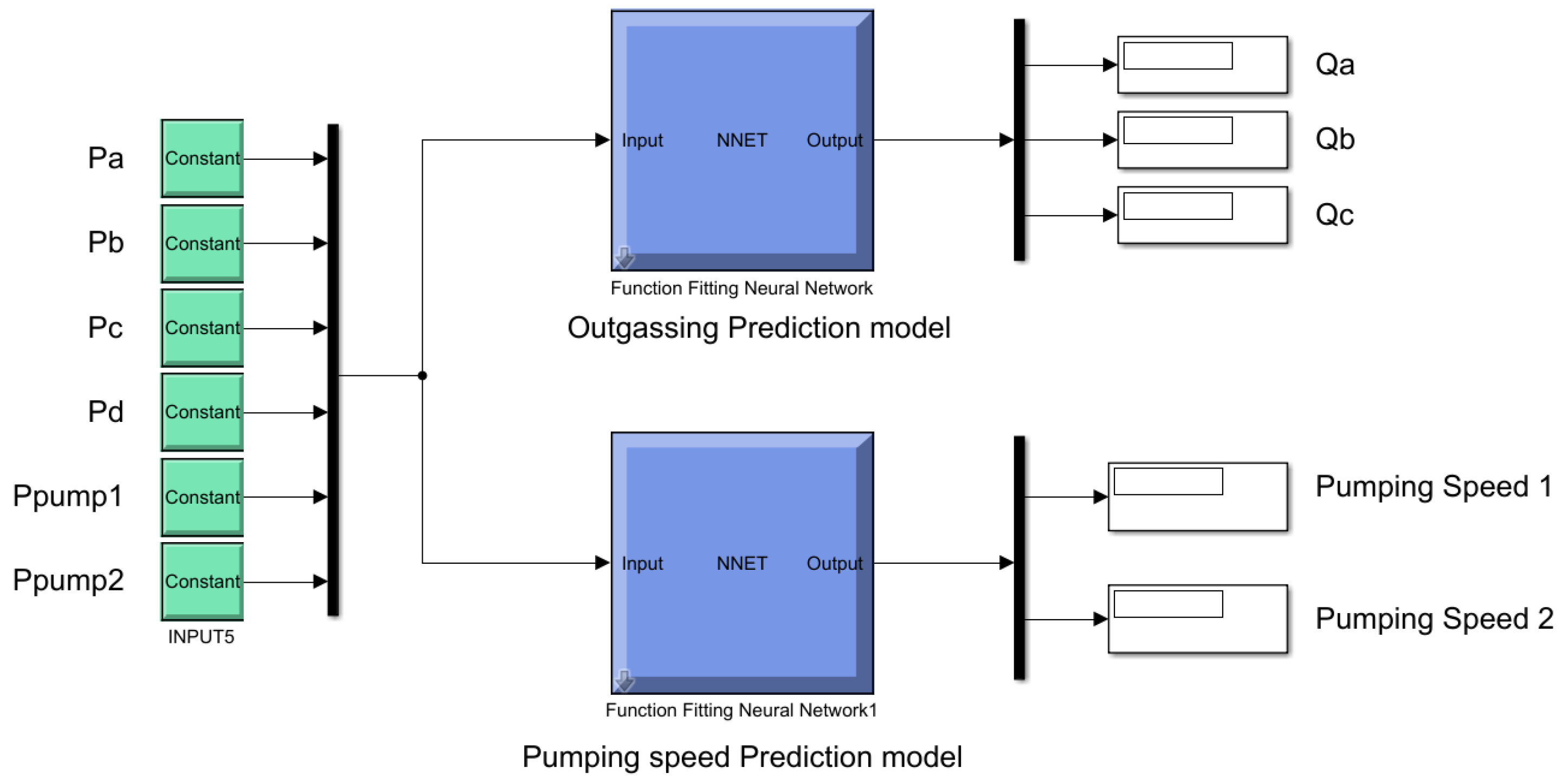
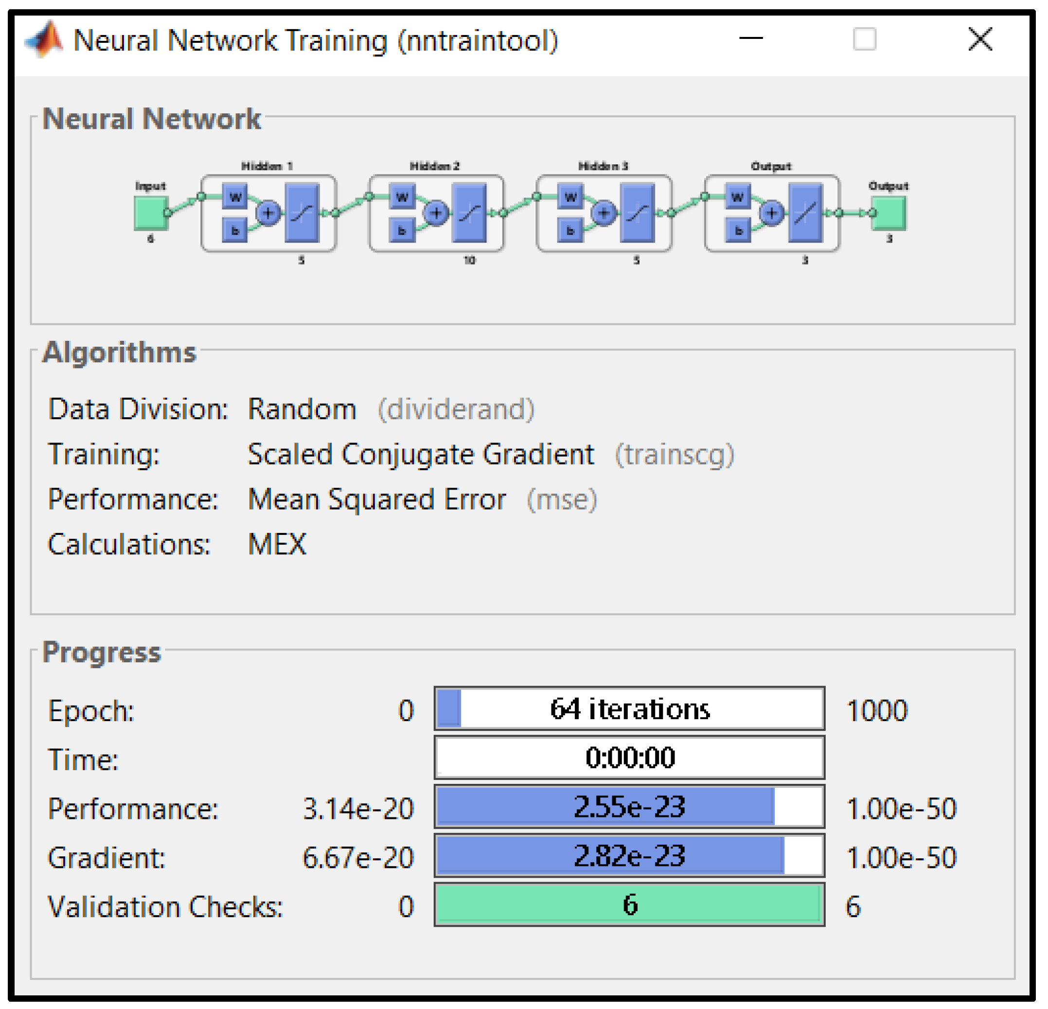
4.2.2. Select Architecture and Training the Network
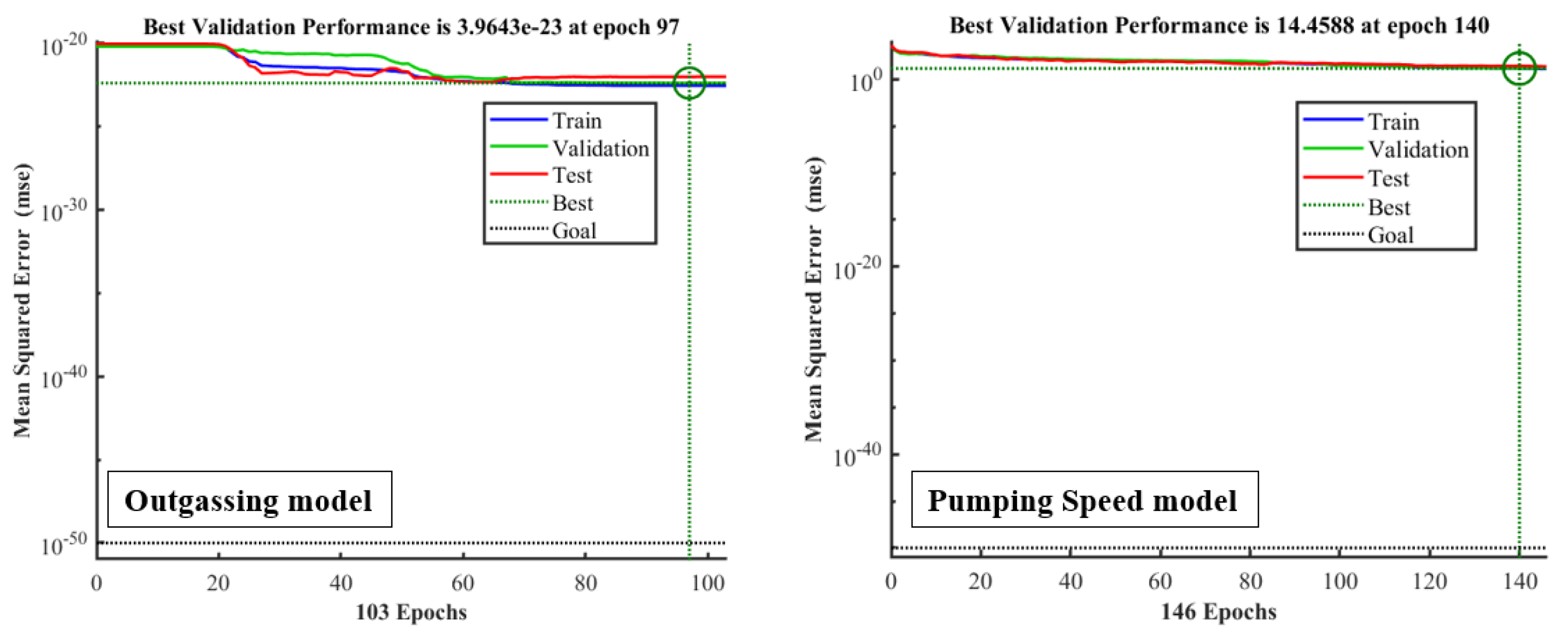
4.2.3. Analysis of Estimation Model Performance
5. Conclusions
Author Contributions
Funding
Data Availability Statement
Acknowledgments
Conflicts of Interest
References
- Sujitjorn, S. Thai Synchrotron Facility: It’s Past and Present. Suranaree J. Sci. Technol. 2015, 22, 227–230. [Google Scholar]
- Grabski, M. Vacuum Technology for Particle Accelerators; Introduction to Accelerator Physics; CERN Accelerator School: Budapest, Hungary, 2016. [Google Scholar]
- Li, Y.; Liu, X. Vacuum Systems Engineering; Vacuum Science and Technology for Accelerator Vacuum Systems; Cornell University: Ithaca, NY, USA, 2015. [Google Scholar]
- Akram, H.M. Selection of Precise Vacuum Pumps for Systems with Diverse Vacuum Ranges. Glob. J. Res. Eng. 2014, 14, 645–651. [Google Scholar]
- Bertolini, L. Ion Pumps. Presented at The U.S. Particle Accelerator School, Lawrence Livermore National Laboratory, 10–14 June 2002. Available online: https://uspas.fnal.gov/materials/02Yale/05_IonPumps.pdf (accessed on 1 January 2023).
- Polozov, S.; Dyubkov, V.; Panishev, A.; Shatokhin, V. Vacuum Condition Simulations for Vacuum Chambers of Synchrotron Radiation Source. In Proceedings of the 27th Russian Particle Accelerator Conference, Alushta, Russia, 27 September–1 October 2021. [Google Scholar] [CrossRef]
- Dong, C.; Mehrotrat, P.; Myneni, G.R. Several Technical Measures to Improve Ultra-High and Extreme-High Vacuum; UNT Libraries Government Documents Department: Denton, TX, USA, 2002; pp. 1–6. [Google Scholar]
- Suetsugu, Y. Numerical Calculation of an Ion Pump’s Pumping Speed; Elsevier Ltd.: Amsterdam, The Netherlands, 1995; Volume 46, pp. 105–111. [Google Scholar]
- Geng, J.; Wang, X.; Guo, M.; Zhang, S.; Cheng, Y.; Li, Y.; Li, H.; Ren, Z. Research on Measuring Method of Pumping Speed for Miniature Sputter Ion Pump. Measurement 2022, 190, 110736. [Google Scholar] [CrossRef]
- Dolcino, L.; Mura, M.; Paolini, C. 50 Years of Varian Sputter Ion Pumps and New Technologies; Elsevier Ltd.: Amsterdam, The Netherlands, 2010; Volume 84, pp. 677–684. [Google Scholar]
- Tsipenyuk, D.Y. Vacuum Technology. Physical Methods, Instruments, and Measurements; Russian Academy of Sciences: Moscow, Russia, 2009; Volume 3, pp. 305–326. ISBN 978-1-905839-56-8. [Google Scholar]
- Calcatelli, A.; Bergoglio, M.; Mohan, P.; Spagnol, M.; Simon, M.D. Study of Outgassing of Sputter-Ion Pump Materials Treated with Three Different Cleaning Procedures; Elsevier Ltd.: Amsterdam, The Netherlands, 1996; Volume 47, pp. 723–726. [Google Scholar]
- Ady, M. Monte Carlo Simulations of Ultra High Vacuum and Synchrotron Radiation for Particle Accelerators. Ph.D. Thesis, École Polytechnique Fédérale de Lausanne, Lausanne, Switzerland, 2016. [Google Scholar]
- Wang, G.; Zhang, S.; Chen, C.; Tang, N.; Lang, J.; Xie, Y. Vacuum System Optimization for EAST Neutral Beam Injector. Energies 2022, 15, 264. [Google Scholar] [CrossRef]
- Shen, S.; Tung, L.; Kishiyama, K.; Nederbragt, W. Design and Analysis of Vacuum Pumping Systems for Spallation Neutron Source Drift-Tube Linac and Coupled-Cavity Linac. In Proceedings of the 2001 Particle Accelerator Conference, Chicago, IL, USA, 18–22 June 2001. [Google Scholar]
- Odngam, S.; Preecha, C.; Sanwong, P.; Thongtan, W.; Srisertpol, J. Precision Analysis and Design of Rotating Coil Magnetic Measurements System. Appl. Sci. 2020, 10, 8454. [Google Scholar] [CrossRef]
- Prawanta, S.; Srisertpol, J. Plane Stabilization of the Electron Storage Ring Using Automatic 3-DOF Girder System. Int. J. Mech. Mechatron. Eng. 2018, 18, 35–44. [Google Scholar]
- Yachum, N.; Chunjarean, S.; Russamee, N.; Srisertpol, J. Parameter Optimization of Hole-Slot-Type Magnetron for Controlling Resonant Frequency of Linear Accelerator 6 MeV by Reverse Engineering Technique. Appl. Sci. 2021, 11, 2384. [Google Scholar] [CrossRef]
- Nguyen, H.T.; Prasad, N.R.; Walker, C.L.; Walker, E.A. A First Course in Fuzzy and Neural Control, 1st ed.; Chapman and Hall/CRC: Boca Raton, FL, USA, 2002. [Google Scholar] [CrossRef]
- Ibrahim, A.M. Fuzzy Logic for Embedded Systems Applications. In Fuzzy Logic for Embedded Systems Applications, 1st ed.; Elsevier: Amsterdam, The Netherlands, 2003; ISBN 9780080469904. [Google Scholar]
- Wu, H.N.; Reliable, L.Q. Fuzzy Control for Continuous-Time Nonlinear Systems with Actuator Faults. IEEE Trans. Syst. Man Cybern. Part B Cybern. 2004, 34, 1743–1752. [Google Scholar] [CrossRef] [PubMed]
- Somwanshi, D.; Bundele, M.; Kumar, G.; Parashar, G. Comparison of Fuzzy-PID and PID Controller for Speed Control of DC Motor Using LabVIEW. Procedia Comput. Sci. 2019, 152, 252–260. [Google Scholar] [CrossRef]
- Ma, F. An Improved Fuzzy PID Control Algorithm Applied in Liquid Mixing System. In Proceedings of the 2014 IEEE International Conference on Information and Automation (ICIA), IEEE, Hailar, China, 28–30 July 2014; pp. 587–591. [Google Scholar] [CrossRef]
- Srisertpol, J.; Numanoy, N.; Pewmaikam, C. PI Controller plus Adaptive Fuzzy Logic Compensator for Torque Controlled System of DC Motor. In Proceedings of the 3rd International Conference on Engineering and Applied Science (2013 ICEAS), Osaka, Japan, 7–9 November 2013. [Google Scholar]
- Patel, H.R.; Shah, V.A. Fuzzy Logic Based Metaheuristic Algorithm for Optimization of Type-1 Fuzzy Controller: Fault-Tolerant Control for Nonlinear System with Actuator Fault. IFAC-PapersOnLine 2022, 55, 715–721. [Google Scholar] [CrossRef]
- Tan, J.H.; Tan, T.S.; Chia Hiik, K.L.; Mat Saad, A.Z.; Malik, S.A. Two-N Input Output Mapping Relationship Fuzziness Adaptation Approach for Fuzzy Based Negative Pressure Wound Therapy System. Expert Syst. Appl. 2022, 208, 118206. [Google Scholar]
- Bähr, P.R.; Lang, B.; Ueberholz, P.; Ady, M.; Kersevan, R. Development of a Hardware-Accelerated Simulation Kernel for Ultra-High Vacuum with Nvidia RTX GPUs. Int. J. High Perform. Comput. Appl. 2022, 36, 141–152. [Google Scholar] [CrossRef]
- Ahmed, S.; Sunil, S.; Mukherjee, S. A Study on Benchmarking of Molflow for Ultra High Vacuum (UHV) System; Institute for Plasma Research: Gandhinagar, India, 2020. [Google Scholar]
- Carter, J. Design and Analysis of Accelerator Vacuum Systems with SynRad and MolFlow+. Mechanical Engineer, AES-MED Group, Argonne National Laboratory, 2015. Available online: https://www.aps.anl.gov/files/APS-Uploads/ASDSeminars/2015/2015-09-02-Carter.pdf (accessed on 1 January 2023).
- Ady, M.; Kersevan, R. Introduction to the Latest Version of the Test-Particle Monte Carlo Code Molflow. In Proceedings of the IPAC2014: 5th International Particle Accelerator Conference, Beijing, China, 15–20 June 2014; pp. 2348–2350. [Google Scholar]
- Rachmatullah, M.I.C.; Santoso, J.; Surendro, K. Determining the number of hidden layer and hidden neuron of neural network for wind speed prediction. PeerJ Comput. Sci. 2021, 7, e724. [Google Scholar] [CrossRef] [PubMed]
- Koutsoukas, A.; Monaghan, K.J.; Li, X.; Huan, J. Deep-learning: Investigating deep neural networks hyper-parameters and comparison of performance to shallow methods for modeling bioactivity data. J. Cheminform. 2017, 9, 42. [Google Scholar] [CrossRef] [PubMed] [Green Version]
- Yan, Z.; Klochkov, Y.; Xi, L. Improving the Accuracy of a Robot by Using Neural Networks (Neural Compensators and Nonlinear Dynamics). Robotics 2022, 11, 83. [Google Scholar] [CrossRef]
- Macaulay, M.O.; Shafiee, M. Machine learning techniques for robotic and autonomous inspection of mechanical systems and civil infrastructure. Auton. Intell. Syst. 2022, 2, 8. [Google Scholar] [CrossRef]
- Lishner, I.; Shtub, A. Using an Artificial Neural Network for Improving the Prediction of Project Duration. Mathematics 2022, 10, 4189. [Google Scholar] [CrossRef]
- Abdulla, M.B.; Herzallah, R.O.; Hammad, M.A. Pipeline Leak Detection Using Artificial Neural Network: Experimental Study. In Proceedings of the 2013 International Conference on Modelling, Identification and Control, ICMIC, Cairo, Egypt, 31 August–2 September 2013; pp. 328–332.
- Shen, S.; Lu, H.; Sadoughi, M.; Hu, C.; Nemani, V.; Thelen, A.; Webster, K.; Darr, M.; Sidon, J.; Kenny, S. A physics-informed deep learning approach for bearing fault detection. Eng. Appl. Artif. Intell. 2021, 103, 104295. [Google Scholar] [CrossRef]
- Castro, O.; Castejón, C.; Garcia-Prada, J.C. Bearing Fault Diagnosis Based on Neural Network Classification and Wavelet Transform. In Proceedings of the 6th WSEAS International Conference on Wavelet Analysis & Multirate Systems, Bucharest, Romania, 16–18 October 2006; Volume 2, pp. 16–18. [Google Scholar]
- Zhao, W.; Egusquiza Estévez, E.; Valero Ferrando, M.d.C.; Egusquiza Montagut, M.; Valentín Ruiz, D.; Presas Batlló, A. A Novel Condition Monitoring Methodology Based on Neural Network of Pump-Turbines with Extended Operating Range. In Proceedings of the 16th IMEKO TC10 Conference on Testing, Diagnostics & Inspection as a Comprehensive Value Chain for Quality & Safety, Berlin, Germany, 3–4 September 2019; IMEKO: Barcelona, Spain, 2019; pp. 154–159. ISBN 9299008418. [Google Scholar]
- Berman, A. Vacuum Engineering Calculations, Formulas, and Solved Exercises; Academic Press, Inc.: Cambridge, MA, USA, 1992; ISBN 0120924552. [Google Scholar]
- Kersevan, R.; Ady, M. TE-VSC-SCC Training Using Molflow for Sputtering Simulations. CERN, 2020. Available online: https://molflow.web.cern.ch/sites/default/files/scc_training_2020/molflow_for_sputtering.pdf (accessed on 1 January 2023).
- Ady, M.; Kersevan, R. MolFlow+ User Guide for Version 2.4. CERN. (2014). Available online: https://molflow.web.cern.ch/sites/default/files/molflow_user_guide.pdf (accessed on 1 January 2023).


| No. | Name | Specification | Quantity |
|---|---|---|---|
| 1 | Scroll Vacuum Pump | - 0.4 kW, 50 Hz - 250 L/min (4.2 L/s), 1.2−2 torr | 1 |
| 2 | Helium Leak Detector | - 2.5 L/s helium pumping speed - Minimum detectable leakage rate for helium 10−13 Pa m3/s | 1 |
| 3 | Thermocouple | - Type K | 5 |
| 4 | Turbo-Molecular Pump | - 1000 RPM, 0.4 A, 220 V | 1 |
| 5 | NI USB-TC01 | - Type J, K, R, S, T, N, E and B thermocouple | 5 |
| 6 | Vacuum Chamber 1 | - D = 146 mm, H = 310 mm | 1 |
| 7 | Sputter-Ion Pump | - Star cell, 500 L/s, typically 3–7 kV - pressures as low as 10−11 mbar | 2 |
| 8 | Vacuum Pipe | - L = 1000 mm, D = 65 mm | 1 |
| 9 | Pfeiffer Vacuum TPG 300 Pressure Gauge | - Measures Pressure from Atmospheric Range, down to 10−11 mbar - Pirani gauges/ Cold cathode gauges | 2 |
| 10 | Vacuum Chamber 2 | - D = 146 mm, H = 285 mm | 1 |
| 11 | Sputter-Ion Pump Controller | - 2 Channels - Output 3000 V–7000 V | 1 |
| 12 | Baking Controller | - Max 10 A, 220 V | 2 |
| 13 | All Metal Angle Valves | - 304 stainless steel - Leak rate < 5–10 mbar.L/s - Temperature operating range from 450° C to −250° C | 4 |
| 14 | Heater | - V = 240 V, p = 170 W, L = 1.5 m | 5 |
| 15 | Ionization Gauge | - Bakeout temp ≤ 250 °C - Measuring range 5 × 10⁻³ to 1 × 10⁻¹¹ mbar | 4 |
| 16 | MOXA | - UPort 1110 V1.4.1, 5 VDC | 3 |
| 17 | RS-232 | 3 | |
| 18 | Computer | - Intel® Core™ i9-9900 CPU @3.1 GHz - RAM 32 GB, 64 bit | 1 |
| 19 | Helium Gas | 1 |
| Range of Vacuum Pressure | Minimum Pressure (Torr) | Maximum Pressure (Torr) |
|---|---|---|
| Low Vacuum (LV) | ||
| Medium Vacuum (MV) | ||
| High Vacuum (HV) | ||
| Very High Vacuum (VHV) | ||
| Ultra-High Vacuum (UHV) | ||
| Extreme-High Vacuum (XHV) | ||
| V | Equation (Mbar) | R2 | Pumping Speed | Pchamber | ||
|---|---|---|---|---|---|---|
| (%) | L/s | P (Mbar) | P (Torr) | |||
| 3000 | y = 5.525ln(x) + 179.91 | 0.9733 | 48–72 | 240–360 | 6 × 10⁻¹¹–5 × 10⁻⁹ | 4.5 × 10⁻¹¹–3.75 × 10⁻⁹ |
| 5000 | y = 4 ×1022x3 − 9 ×1015x2 + 5×10⁸x + 71.053 | 0.9044 | 72–76 | 360–380 | 5 × 10⁻⁹–1 × 10⁻⁷ | 3.75 × 10⁻⁹–7.5 × 10⁻⁸ |
| 7000 | y = 10.52ln(x) + 246.07 | 0.9816 | 76–99 | 380–495 | 1 × 10⁻⁷–1 × 10⁻⁶ | 7.5 × 10⁻⁸–7.5 × 10⁻⁷ |
| V | Equation (Mbar) | R2 | Pumping Speed (%) | Controller | |
|---|---|---|---|---|---|
| P (Mbar) | P (Torr) | ||||
| 3000 | y = 4.3486ln(x) + 156.73 | 0.9732 | 64–72 | 6.2 × 10⁻¹⁰–5 × 10⁻⁹ | 4.65 × 10⁻¹⁰–3.75 × 10⁻⁹ |
| 4000 | y = 8 × 10⁸x + 68.048 | 0.9973 | 72–76 | 5 × 10⁻⁹–1 × 10⁻⁸ | 3.75 × 10⁻⁹–7.5 × 10⁻⁹ |
| 5000 | y = 2.1615ln(x) + 115.97 | 0.9709 | 76–79 | 1 × 10⁻⁸–4 × 10⁻⁸ | 7.5 × 10⁻⁹–3× 10⁻⁸ |
| 6000 | y = 4.5108ln(x) + 155.92 | 0.9784 | 79–83.5 | 4 × 10⁻⁸–2 × 10⁻⁷ | 3 × 10⁻⁸–1.5 × 10⁻⁷ |
| 7000 | y = 10.52ln(x) + 246.07 | 0.9816 | 83.5–99 | 2 × 10⁻⁷–1 × 10⁻⁶ | 1.5 × 10⁻⁷–7.5 × 10⁻⁷ |
| No. | Pressure Input (Torr) | Input Variable | Output Variable 1 | Output Variable 2 | Percent Variable | Voltage Supply 1 | Voltage Supply 2 |
|---|---|---|---|---|---|---|---|
| 1 | ≤3.75 × 10⁻⁹ | N | L | L2 | 0 | 3000 | 3000 |
| 2 | 3.751 × 10⁻⁹–7.5 × 10⁻⁹ | SN | SL | SL2 | 25 | 4000 | 4000 |
| 3 | 7.51 × 10⁻⁹–3 × 10⁻⁸ | Z | M | M2 | 50 | 5000 | 5000 |
| 4 | 3.01 × 10⁻⁸–1.506 × 10⁻⁷ | SP | SH | SH2 | 75 | 6000 | 6000 |
| 5 | ≥1.507 × 10⁻⁷ | P | H | H2 | 100 | 7000 | 7000 |
| %Outgassing Rate | Q (mbar. L/s) | Pc (mbar) | Pi (mbar) |
|---|---|---|---|
| −15% | 2.975 × 10⁻¹¹ | 2.55 × 10⁻¹⁰ | 1.97 × 10⁻¹⁰ |
| −10% | 3.15 × 10⁻¹¹ | 2.70 × 10⁻¹⁰ | 2.09 × 10⁻¹⁰ |
| −5% | 3.325 × 10⁻¹¹ | 2.86 × 10⁻¹⁰ | 2.21 × 10⁻¹⁰ |
| normal | 3.5 × 10⁻¹¹ | 3 × 10⁻¹⁰ | 2.32 × 10⁻¹⁰ |
| 5% | 3.675 × 10⁻¹¹ | 3.15 × 10⁻¹⁰ | 2.44 × 10⁻¹⁰ |
| 10% | 3.85 × 10⁻¹¹ | 3.31 × 10⁻¹⁰ | 2.56 × 10⁻¹⁰ |
| 15% | 4.025 × 10⁻¹¹ | 3.45 × 10⁻¹⁰ | 2.67 × 10⁻¹⁰ |
| %x | Red Line Axial Pressure | Green Line Axial Pressure | Blue Line Axial Pressure | |||
|---|---|---|---|---|---|---|
| x (mm) | P (10−10 Mbar) | x (mm) | P (10−10 Mbar) | x (mm) | P (10−10 Mbar) | |
| 0 | 0 | 2.32 | 0.00 | 3 | 0.00 | 3.03 |
| 0.05 | 14.25 | 2.38 | 9.70 | 3 | 13.65 | 3.01 |
| 0.10 | 28.50 | 2.43 | 19.40 | 2.98 | 27.30 | 2.96 |
| 0.15 | 42.75 | 2.47 | 29.10 | 2.95 | 40.95 | 2.89 |
| 0.20 | 57.00 | 2.51 | 38.80 | 2.9 | 54.60 | 2.79 |
| 0.25 | 71.25 | 2.55 | 48.50 | 2.82 | 68.25 | 2.76 |
| 0.30 | 85.50 | 2.58 | 58.20 | 2.77 | 81.90 | 2.75 |
| 0.35 | 99.75 | 2.61 | 67.90 | 2.76 | 95.55 | 2.75 |
| 0.40 | 114.00 | 2.64 | 77.60 | 2.76 | 109.20 | 2.75 |
| 0.45 | 128.25 | 2.67 | 87.30 | 2.76 | 122.85 | 2.75 |
| 0.50 | 142.50 | 2.69 | 97.00 | 2.76 | 136.50 | 2.75 |
| 0.55 | 156.75 | 2.73 | 106.70 | 2.76 | 150.15 | 2.75 |
| 0.60 | 171.00 | 2.76 | 116.40 | 2.76 | 163.80 | 2.77 |
| 0.65 | 185.25 | 2.78 | 126.10 | 2.76 | 177.45 | 2.81 |
| 0.70 | 199.50 | 2.78 | 135.80 | 2.76 | 191.10 | 2.91 |
| 0.75 | 213.75 | 2.78 | 145.50 | 2.76 | 204.75 | 3.07 |
| 0.80 | 228.00 | 2.78 | 155.20 | 2.76 | 218.40 | 3.21 |
| 0.85 | 242.25 | 2.78 | 164.90 | 2.76 | 232.05 | 3.33 |
| 0.90 | 256.50 | 2.78 | 174.60 | 2.76 | 245.70 | 3.45 |
| 0.95 | 270.75 | 2.78 | 184.30 | 2.76 | 259.35 | 3.56 |
| 1.00 | 285.00 | 2.78 | 194.00 | 2.76 | 273.00 | 3.63 |
| Data Measuring from an Instrument of the Experimental | Outgassing Prediction from ANN | |||||||
|---|---|---|---|---|---|---|---|---|
| Pa | Pb | Pc | Pd | Ppump1 | Ppump2 | Qa | Qb | Qc |
| 9.0659 × 10⁻¹⁰ | 1.8665 × 10⁻⁹ | 2.2665 × 10⁻⁹ | 2.5331 × 10⁻⁹ | 5.8662 × 10⁻¹⁰ | 1.7332 × 10⁻⁹ | 5.89 × 10⁻¹¹ | 2.63 × 10⁻¹¹ | 3.13 × 10⁻¹⁰ |
| 8.3993 × 10⁻¹⁰ | 1.7332 × 10⁻⁹ | 2.2665 × 10⁻⁹ | 2.3998 × 10⁻⁹ | 6.1328 × 10⁻¹⁰ | 1.7332 × 10⁻⁹ | 5.83 × 10⁻¹¹ | 2.24 × 10⁻¹¹ | 3.11 × 10⁻¹⁰ |
| 1.0399 × 10⁻⁹ | 1.8665 × 10⁻⁹ | 2.3998 × 10⁻⁹ | 2.5331 × 10⁻⁹ | 5.0662 × 10⁻¹⁰ | 1.8665 × 10⁻⁹ | 5.88 × 10⁻¹¹ | 2.43 × 10⁻¹¹ | 3.05 × 10⁻¹⁰ |
| 9.1992 × 10⁻¹⁰ | 1.8665 × 10⁻⁹ | 2.2665 × 10⁻⁹ | 2.5331 × 10⁻⁹ | 6.5328 × 10⁻¹⁰ | 1.7332 × 10⁻⁹ | 5.97 × 10⁻¹¹ | 2.84 × 10⁻¹¹ | 3.11 × 10⁻¹⁰ |
| Experimental Results for Determining the Pumping Speed and Root Mean Square Error | |||||
|---|---|---|---|---|---|
| Calculation | ANN | RMSE | |||
| Spump1 | Spump2 | Spump1 | Spump2 | Ppump1 | Ppump2 |
| 312.34 | 342.26 | 253.33 | 266.00 | 9.84804 × 10⁻²² | 7.53585 × 10⁻²¹ |
| 313.56 | 342.26 | 242.81 | 272.79 | 5.95539 × 10⁻²³ | 2.82551 × 10⁻²² |
| 308.29 | 344.31 | 249.88 | 268.52 | 1.15294 × 10⁻²⁰ | 1.35753 × 10⁻²⁰ |
| 315.31 | 342.26 | 239.84 | 273.63 | 5.96047 × 10⁻²³ | 1.35492 × 10⁻²¹ |
Disclaimer/Publisher’s Note: The statements, opinions and data contained in all publications are solely those of the individual author(s) and contributor(s) and not of MDPI and/or the editor(s). MDPI and/or the editor(s) disclaim responsibility for any injury to people or property resulting from any ideas, methods, instructions or products referred to in the content. |
© 2023 by the authors. Licensee MDPI, Basel, Switzerland. This article is an open access article distributed under the terms and conditions of the Creative Commons Attribution (CC BY) license (https://creativecommons.org/licenses/by/4.0/).
Share and Cite
Seangsri, S.; Wanglomklang, T.; Khaewnak, N.; Yachum, N.; Srisertpol, J. Optimizing Ultra-High Vacuum Control in Electron Storage Rings Using Fuzzy Control and Estimation of Pumping Speed by Neural Networks with Molflow+. Systems 2023, 11, 116. https://doi.org/10.3390/systems11030116
Seangsri S, Wanglomklang T, Khaewnak N, Yachum N, Srisertpol J. Optimizing Ultra-High Vacuum Control in Electron Storage Rings Using Fuzzy Control and Estimation of Pumping Speed by Neural Networks with Molflow+. Systems. 2023; 11(3):116. https://doi.org/10.3390/systems11030116
Chicago/Turabian StyleSeangsri, Soontaree, Thanasak Wanglomklang, Nopparut Khaewnak, Nattawat Yachum, and Jiraphon Srisertpol. 2023. "Optimizing Ultra-High Vacuum Control in Electron Storage Rings Using Fuzzy Control and Estimation of Pumping Speed by Neural Networks with Molflow+" Systems 11, no. 3: 116. https://doi.org/10.3390/systems11030116