1. Introduction
Traffic sensors represent a critical component in the ongoing evolution of Intelligent Transportation Systems (ITS) and provide essential data sources that can be leveraged by modern and emerging AI systems to revolutionize traffic management and the strategic planning of our vast highway networks. The significance of these sensors cannot be overstated as they offer crucial insights into traffic patterns, congestion levels, and dynamic road conditions, all of which are instrumental in optimizing traffic flow and enhancing overall road safety. However, as the role of traffic sensors in modern transportation infrastructure becomes increasingly important, so do the substantial challenges that come with their widespread deployment. These obstacles can range from the pragmatic constraints of limited budgets to the intricacies of selecting appropriate sensor types and dealing with the inherent possibility of sensor failures [
1]. The quest to enhance the observability of traffic flow, a crucial objective within the realm of ITS, necessitates the creation of extensive sensor networks that can span vast geographical areas. This expansive network, while undeniably powerful in its capacity to capture comprehensive traffic data, brings with it the need for substantial initial investments for deployment and continuous, labor-intensive maintenance. These formidable financial and operational burdens pose a significant obstacle to the practical implementation of large traffic sensor networks.
It is in addressing these challenges that the Traffic Sensor Location Problem (TSLP) emerges as a critical focal point for transportation researchers and planners. This problem encapsulates the intricate process of strategically placing traffic sensors to maximize their utility while minimizing the financial and operational burdens associated with their maintenance and upkeep. Over the past few decades, extensive research has been devoted to tackling the TSLP, resulting in a diverse range of proposed methods. These approaches can be broadly classified into six categories [
2]: O/D estimation [
3,
4], flow observability [
5], link flow inference [
6,
7,
8], path reconstruction [
9], traffic surveillance [
10], and travel time estimation [
11]. Our proposed framework in this paper is related to flow observability and link low inference, while emphasizing the overall network coverage. Given the nature of the problem, which involves binary-choice decision for each candidate location, the most popular approaches center on constructing and solving mixed-integer linear or nonlinear programs. However, their practical utility in dealing with intricate, extensive real-world highway networks is frequently constrained by distinct challenges [
12], such as the exceedingly high computational complexity associated with a large number of edges and nodes. For instance, with a network of n links, the TSLP search space is 2n for a single sensor. In large metropolitan regions, the highway network can rapidly expand to encompass tens of thousands of links, rendering the traditional approach unviable. In the context of this study, our objective is to harness data directly from regional transportation planning models and address the TSLP through a novel data-driven approach by leveraging information theory and maximizing information gain in a low-dimensional embedding (vector) space that jointly captures complex network topology and pertinent segment-level features. As such, the proposed framework is well suited for parallel, scalable computation with modern graphics processing units (GPUs) or tensor processing units (TPUs) for large-scale, real-world highway networks.
2. Methods
Our proposed framework is depicted in
Figure 1. Firstly, we abstract the study highway network as a directional graph, where each segment is treated as a node. Then, we obtain the topological embedding of the graph in a vector space, where each node (segment) is represented by a dense vector in R
n while preserving the network topology. To enhance the topological embedding, we introduce additional dimensions (
Rm) to account for segment-specific features such as AADT, functional class, and the number of lanes. This dimensional augmentation results in a joint vector space (
R(n+m)), highlighted by the shaded blue box in
Figure 1. As a result, the inherent distance metric between two nodes (or segments) in this joint vector space incorporates both their topological relationship and segment attributes.
Subsequently, we model the node (segment) distribution of the network in this joint vector space using kernel density estimation (KDE), which is referred to as model distribution, denoted by Q(x). On the other hand, the choice set of the proposed sensor locations (segments), together with existing sensor locations, represents the data distribution of the segments with a sensor, denoted by P(x). By such construct, the TSLP is formulated as an optimization problem that minimizes the discrepancy between P(x) and Q(x), such as Kullback–Leibler (KL) divergence, with respect to the proposed sensor locations. Notably, this formulation presents a distinctive perspective compared to the common machine learning scenario, wherein the data distribution (P(x)) is known and the objective is to train the model (Q(x)) to align with the data. To effectively address this problem, we developed a customized genetic algorithm integrated with physics-guided random walks (PGRW) that operate from the existing sensor locations. This combination serves to effectively reduce the search space for determining the optimal locations for new sensors.
To set up the stage for coherent presentation, we delineate the process into six key components: (1) Graph Representation of Highway Network, (2) Topological Embedding of Graph, (3) Construction of Joint Vector Space, (4) Kernel Density Estimation, (5) Optimization Problem Formulation, and (6) Solution Algorithm. Throughout our discussion, we utilize the Savannah highway network as an illustrative example to facilitate a comprehensive understanding of the process.
Each of the six components is discussed in detail subsequently with a dedicated subsection.
2.1. Graph Representation of Highway Network
This initial step involves the representation of a highway network as a graph to capture its topology. For demonstration, the Savannah highway network is used, which consists of 1616 segments with different functional classes, such as interstate highways, arterials, collectors, and local roads. The GIS visualization of the network is shown in
Figure 2. The green dots indicate the locations of the 26 existing Continuous Count Stations (CCSs). In this paper, sensor locations refer to CCSs.
Both the undirected graph and the directed graph are constructed and shown in
Figure 3. Each node in the graph represents a road segment in the original highway network. To capture the directional traffic flows, the directed graph is adopted in this study.
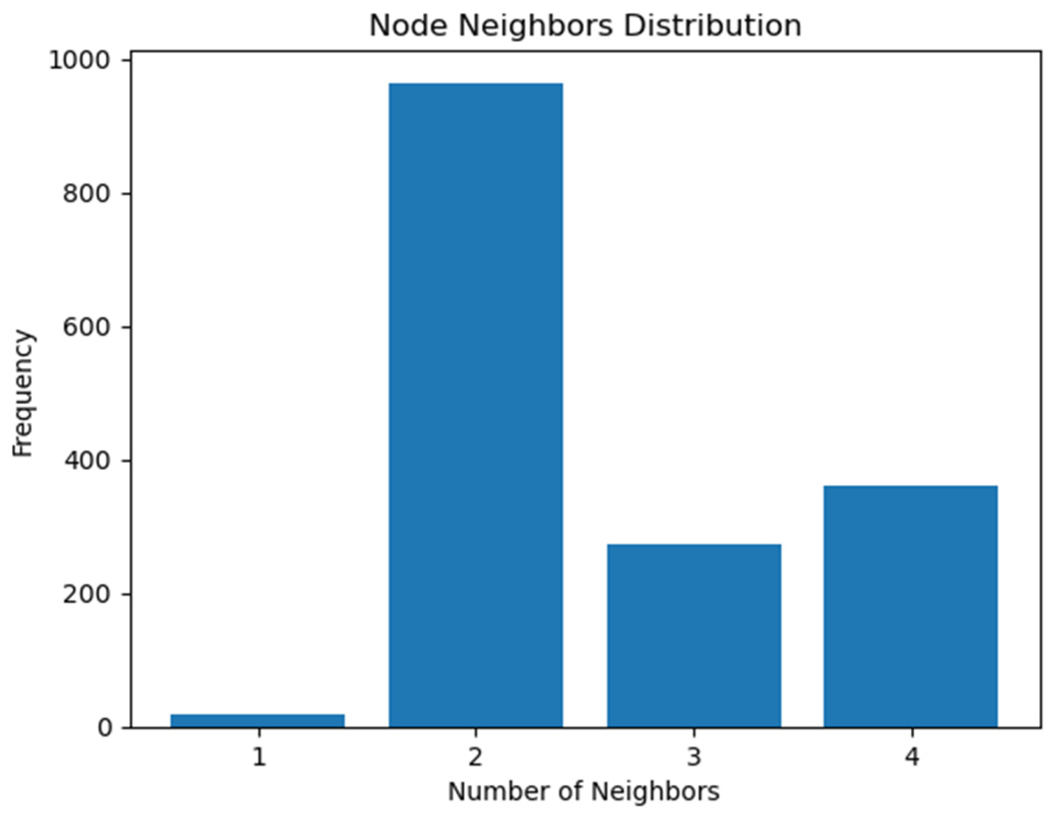
A straightforward way of assessing the overall topology of a highway network is to examine the distribution of the number of neighboring segments. As depicted in
Figure 4, most segments demonstrate connections with two neighbors, followed by segments with four and three neighbors. The few segments with only one neighbor represent endpoints or
cul-de-sac segments.
2.2. Topological Embedding of Graphs
To effectively capture meaningful representations of the directed graph mentioned above, while simultaneously preserving its graph structure properties, we use the Node2Vec embedding method proposed by Grover and Leskovec [
13], which is a scalable learning-based approach for embedding network topology. It harnesses the power of machine learning and embedding techniques to learn vector representations that intricately capture the nuanced relationships between nodes, rendering them highly useful for various downstream tasks in graph analysis. For our implementation, the adopted Node2Vec parameters are shown in
Table 1.
Generally, the parameters
p and
q control the exploration and exploitation behavior when the Node2Vec algorithm starts sampling the graph. Node2Vec uses a 2nd-order random walk and guides the walking process by introducing a search bias α. Refer to Equation (1),
where
denotes the unnormalized transition probability between nodes
and
and
is the static edge weight.
is computed by Equation (2),
where
denotes the shortest path distance between nodes
and
[
13].
When considering the current node v in the context of Node2Vec, two important parameters, p and q, play a significant role in shaping the walker’s behavior. Setting 0 < p < 1 and q > 1 makes the walker more likely to exploit the visited nodes, favoring local exploration, while reducing the likelihood of exploring nodes further away. Conversely, when setting p > 1 and 0 < q < 1, the walker becomes more inclined to visit nodes further away, promoting global exploration behavior. In our case, we intentionally set p = q = 1. The reason behind this choice is that our implementation of the Node2Vec model aims to encode the topology while maximally preserving the graph’s structure without bias towards either local or global aspects.
For visualizing the embeddings produced by Node2Vec, we employ a 3D visualization technique using Uniform Manifold Approximation and Projection (UMAP). The UMAP has proven to be highly effective, offering competitive low-dimensional manifold representation while also preserving more of the global structure of the embeddings [
14]. As depicted in
Figure 5, the UMAP visualization demonstrates a balanced trade-off between local and global connectivity. The current CCS locations are shown as red dots, indicating a representative sampling of network segments in the embedding space.
2.3. Construction of Joint Vector Space
In addition to topology embeddings, explicitly considering segment (node) features becomes important when determining the optimal sensor placement. In practical scenarios, state Departments of Transportation (DOTs) often prioritize achieving a well-balanced network coverage by strategically distributing sensors across various types of facilities and areas. To meet this requirement, we incorporate three important segment features, namely Total Volume, Lanes, and Functional Class, and combine them with the 8-dimensional Node2Vec embeddings, resulting in an expanded 11-dimensional joint feature space. This allows us to create a comprehensive representation that takes into account both the topological characteristics and the specific attributes of individual segments. Furthermore, we apply Min-Max scaling to all feature dimensions of the joint embedding space to ensure they share a consistent scale and contribute equally to the subsequent analysis and decision-making process.
2.4. Kernel Density Estimation
Kernel density estimation (KDE) is a non-parametric method to estimate underlying distribution directly from data samples. Unlike the histogram, the KDE produces smooth estimate of the probability density function by using all sample data points and convincingly reveals multimodality [
15]. Particularly, KDE imposes a kernel, a smooth and symmetric function, at each data point. The density estimation is derived by summing the contributions from these kernels. The choice of kernel and other parameters (e.g., bandwidth) can affect the smoothness of the estimated density. With a dataset of {
, the kernel density estimator can be computed by Equation (3),
where
for all real
x, and
.
K(.) is the kernel and
h > 0 is a smoothing parameter, referred to as bandwidth. h controls the smoothness of the kernel. Improper selection of h can lead to one of two issues: over-smoothing or under-smoothing. Over-smoothing fails to capture the underlying structure of data, and eventually leads to an oversimplified representation of the true distribution, while under-smoothing captures noises in the data and leads to inaccurate representation of the data [
16].
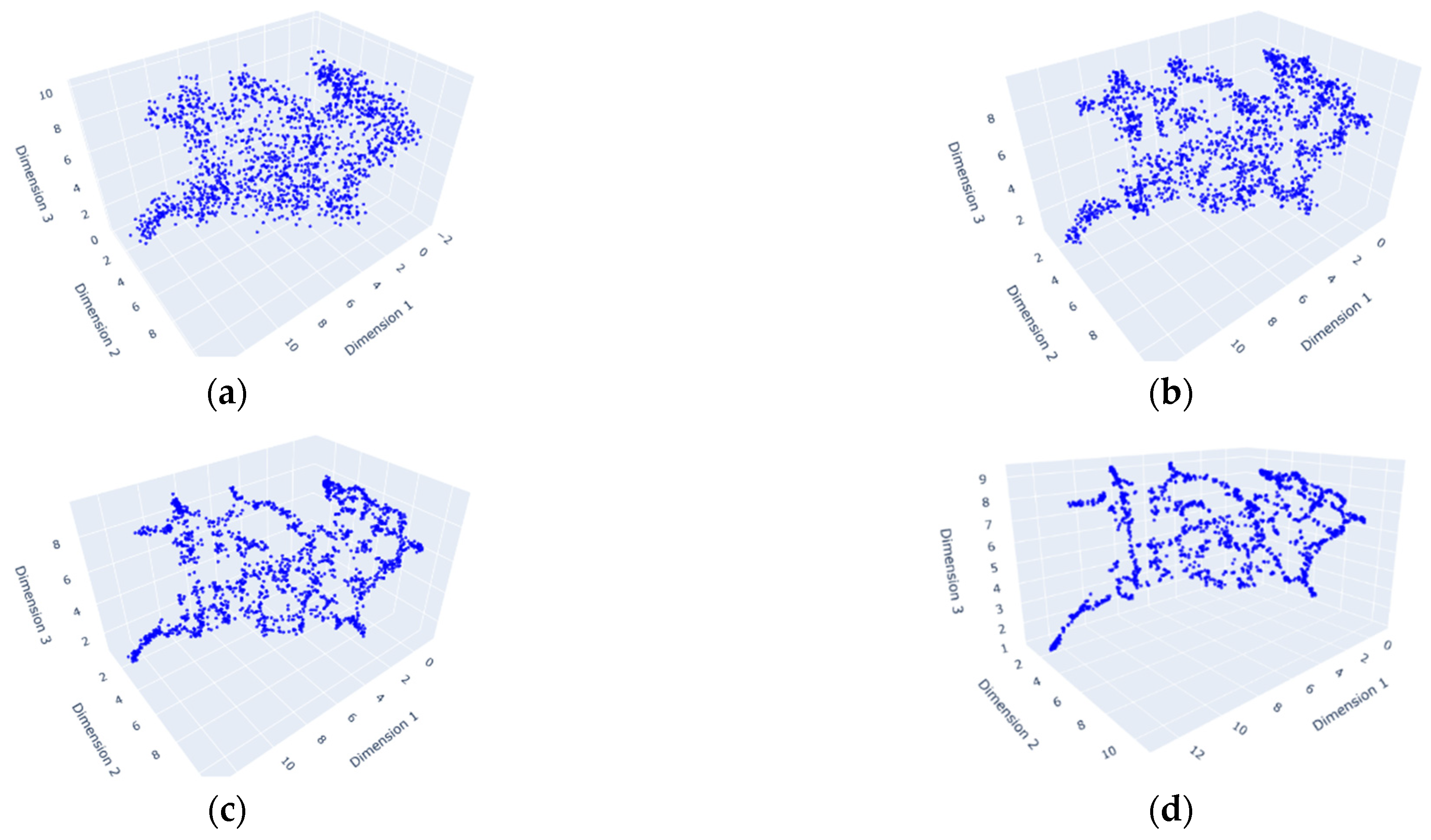
Figure 6 shows the 3D visualization of varying bandwidth values. The bandwidth of 0.4 (
Figure 6a) indicates over-smoothing, while the bandwidth of 0.05 (
Figure 6d) shows under-smoothing. The bandwidth of 0.2 (
Figure 6b) is chosen to capture both local and global structures. Eventually, this KDE serves as the model distribution,
Q(
x), for formulating our optimization problem in the following section.
2.5. Optimization Problem Formulation
Drawing inspiration from information theory, we formulate an optimization problem in the joint embedding space, guided by fundamental principles of information theory. Specifically, we would like our choice set of new sensor locations to maximize the information gain. This is equivalent to minimizing the Kullback–Leibler (
KL) divergence between the data distribution, denoted as
P(
x), and the model distribution, represented as
Q(
x), through KDE. The KL divergence is also known as information divergence and relative entropy, measuring the dissimilarity between two distributions. The KL divergence is computed by Equation (4) for discrete probability distributions
P(
x) and
Q(
x), defined on the same sample space χ [
17].
The model distribution
Q(
x) is estimated based on the outputs (e.g., the loaded network) of a travel demand model. The data distribution
P(
x) represents the choice set of locations (segments) for the existing sensors (
) and the planned sensors (
). The objective is to select the planned sensor sites
to minimize the
KL divergence between
P(
x) and
Q(
x), in the joint embedding space as previously described. Thus, the optimization problem is written in Equation (5),
where
denotes the reduced search space by the PGRW algorithm, which is discussed in the next section.
2.6. Solution Algorithm
In this subsection, we introduce a solution algorithm, which consists of two components: (1) physics-guided random walk and (2) genetic algorithm. The former effectively reduces the search space, while the latter conducts search with penalty handling.
2.6.1. Physics-Guided Random Walk
Given the potentially large solution space for real-world highway networks, it is essential to reasonably narrow down the solution space first. For this purpose, we adopt a random walk-based approach. The idea is to design walkers to start from existing sensor locations, where traffic flows are known. Each walk is guided by traffic flows on the neighboring segments (nodes) subject to the network topology. Through a finite number of walk steps, each walker can cover a part of the network in the vicinity of existing sensors. By viewing traffic flow as a “diffusion process” across a highway network, the visited parts of network by the walkers are considered to be “inferable”, which leave the remaining unvisited parts of the network to be explored for optimal sensor locations. In our implementation, we let multiple walkers start walking at the same time from the current sensor locations, which are 26 for the Savannah highway network.
To align with our intention on flow estimation, we guide all walkers with network traffic flow information, referred to as physics-guided random walk (PGRW) in this paper. The probability of walking to each direct neighbor is computed by the softmax function of Annual Average Daily Traffic (AADT) over all neighboring nodes by Equation (6),
where
k is the number of direct neighbors and
is AADT on segment
i.
In the context of the PGRW algorithm, users have the ability to specify their preferred size for the reduced solution space when seeking optimal sensor locations. As an illustrative example, we opted for a target search space size of 100. The outcomes of the PGRW algorithm are visually presented in
Figure 7, where distinct trajectories, distinguished by triangle markers in varying colors, depict the diverse paths taken by different walkers who started from the existing sensor locations. The presence of blue bubbles on the graph signifies the unexplored segments, which collectively compose the reduced space designated for the exploration of optimal sensor locations. It is important to underscore that the selection of the search space size confers a degree of flexibility, allowing users to strike a balance between computational resource usage and the confidence in achieving global optimality.
2.6.2. Genetic Algorithm
In recent years, a multitude of researchers have proposed various metaheuristic algorithms to tackle real-world problems in engineering, economics, and management, among other fields [
18]. Generally, these algorithms draw inspiration from three primary sources: biological evolution processes, physical laws, and swarm behavior [
19,
20]. Among population-based metaheuristics, a dominant and widely adopted subset, these algorithms iteratively search for optimal solutions by exploring a set of candidate solutions and leveraging population characteristics to guide the search [
21]. An exemplary evolutionary algorithm within this family is the genetic algorithm (GA). In the GA, a population of candidate solutions (individuals) undergoes evolution through biological operators, including selection, crossover, and mutation. The process commences with a randomly generated population of individuals, and in each generation, every individual is evaluated by a fitness function. The individuals with higher fitness scores are retained from the current population and subsequently subjected to crossover and mutation to form a new generation. This iterative process continues until either the maximum fitness score is achieved or the maximum number of generations is reached.
In our setting, a gene is defined as a binary digit, taking the value of either 0 or 1. Each gene represents the selection status of a specific node or segment within the network, determining whether it is chosen for sensor placement. When a gene holds a value of 1, it signifies that the corresponding node or segment is selected for sensor placement, whereas a value of 0 indicates that it is not chosen. By this gene definition, an individual is represented as a binary string comprising candidate nodes or segments eligible for sensor placement. This binary string encapsulates the selection configuration of nodes or segments, with each gene in the string denoting the inclusion or exclusion of the corresponding node or segment for sensor deployment.
We define the fitness function as the reciprocal of KL divergence between model distribution Q(x) and data distribution P(x) as previously introduced.
It should be noted that the standard GA does not impose any restrictions on the number of “1” genes, which represent the segments selected for sensor placement in our setting. In real-world applications, the number of sensors to be installed is typically constrained by a limited budget or other practical considerations. Therefore, achieving a definitive number of sensors is often practically preferable. To ensure that the GA conforms to such a constraint, we employ a penalty trick, which involves pre-filtering candidate solutions that fail to meet the required number of “1” genes prior to fitness evaluation. Non-compliant solutions are assigned a substantial penalty with a low fitness score, effectively discouraging their continued participation in the evolutionary process. The penalty trick preserves the integrity of the GA’s evolution process while respecting the desired constraint on the number of planned sensors. Algorithm 1 shows the implementation of our customized GA.
| Algorithm 1. Pseudocode of GA with penalty trick. |
| 1: Initialize population P with size |
| 2: For generation to : |
| 3: For to : |
| 4: If (the number of “1” gene in individual ) ! = (the desired number of sensors): |
| 5: assign a low fitness score (e.g., 0.00001) to individual . |
| 6: Else: compute the fitness score for individual . |
| 7: End for |
| 8: Select the best m individuals in the population P and save them as population, |
| 9: //crossover operation// |
| 10: For to : |
| 11: randomly select two individuals and from population P |
| 12: generate and by crossover. |
| 13: save and to population |
| 14: End for |
| 15: //mutation operation// |
| 16: For to : |
| 17: select an individual from |
| 18: apply mutation to obtain individual |
| 19: replace with in |
| 20: End for |
| 21: update population |
| 22: End for |
| 23: Return the best individual, in population P |
3. Results
The optimal parameters for the GA were determined through a grid search and are summarized in
Table 2. Notably, for the parent selection process, we employed the roulette wheel method.
The GA is subsequently implemented using the optimal parameters in
Table 2 with the reduced solution space previously generated by the PGRW (
Figure 7). As depicted in
Figure 8, the evolution process demonstrates convergence, with the fitness score approaching stability after approximately 130 evolutions.
For illustrative purposes, consider adding five new sensor sites to the Savanna highway network.
Figure 9 shows the GA identified optimal locations, depicted by blue circles, for installing these new sensors. For comparison, the results derived from the exhaustive search (ES) method are also displayed in
Figure 9, denoted by the red solid dots. Notably, four out of the five locations selected by the GA method align with those of the ES method. Upon closer inspection within the overlapping area in
Figure 9, it becomes evident that the two divergent locations in the zoomed-in view correspond to the same direction of the same extended roadway section, while the matched location is for the other direction. Regarding computational efficiency, the GA method achieved convergence in 8 s, while the ES method took up to 20 h. These experiments were conducted on a laptop equipped with an Intel(R) Core(TM) i7-10870H CPU @ 2.20 GHz, 32 GB RAM, and NVIDIA GeForce RTX3070.
4. Discussion and Conclusions
In this study, we introduce a novel framework designed to tackle the TSLP. Inspired by information theory, our approach harnesses a distinctive fusion of network topology and segment-level features within a unified embedding space to identify optimal sensor locations, maximizing information gain. Unlike previous works, our proposed framework operates in a low-dimensional vector space, facilitating parallel and scalable computation using modern GPUs or TPUs, particularly for large-scale networks.
Employing a GA with penalty handling addresses the optimization challenge with desirable constraints, while the integration of the PGRW algorithm expedites the solution process. This dual approach not only significantly reduces the search space but also strikes a balance between computational load and the confidence of achieving global optimality. For illustration purposes, our framework has been applied to the Savannah highway network. The outcomes align well with those of exhaustive search, but with much faster convergence, demonstrating its potential for application in expansive real-world metropolitan or statewide highway networks.
Nonetheless, it is crucial to emphasize that while the GA serves as our primary solution method, our framework is inherently versatile and not bound to any specific solution algorithms. The pursuit of an optimal solution, as evidenced by the objective of minimizing KL divergence, is fundamentally shaped by the underlying network topology and the construction of the joint embedding space.
However, we acknowledge specific limitations and suggest avenues for future research. Our current investigation focused on three segment features, treating them equally in the joint embedding space. An essential direction for further exploration involves incorporating stakeholder preferences and policy guidance into the optimization framework, enabling a more nuanced consideration of diverse features and their varying contributions. Additionally, a promising research approach entails formulating separate or interconnected optimization problems, especially for different sensor types with distinct purposes. This approach can facilitate a comprehensive planning and deployment strategy for large, hybrid sensor networks, tailored to meet specific objectives and stakeholder requirements.
Author Contributions
Conception and design: J.J.Y.; data processing: Y.Y.; analysis and interpretation of results: Y.Y. and J.J.Y.; draft manuscript preparation: Y.Y.; review and editing: J.J.Y.; visualization, Y.Y.; supervision, J.J.Y.; project administration, J.J.Y.; funding acquisition, J.J.Y. All authors have read and agreed to the published version of the manuscript.
Funding
This research was funded by Georgia Department of Transportation, grant number RP 20-28.
Data Availability Statement
Some or all of the data that support the findings of this study are available from the corresponding author upon reasonable request.
Acknowledgments
The work presented in this project is part of a research project (RP 20-28) sponsored by the Georgia Department of Transportation, United States. The contents of this paper reflect the views of the authors, who are solely responsible for the facts and accuracy of the data, opinions, and conclusions presented herein. The contents may not reflect the views of the funding agency or other individuals. The authors would like to acknowledge the financial support from the Georgia Department of Transportation in the United States.
Conflicts of Interest
The authors declare no conflict of interest.
References
- Salari, M.; Kattan, L.; Lam, W.H.K.; Esfeh, M.A.; Fu, H. Modeling the effect of sensor failure on the location of counting sensors for origin-destination (OD) estimation. Transp. Res. Part C Emerg. Technol. 2021, 132, 103367. [Google Scholar] [CrossRef]
- Owais, M. Traffic sensor location problem: Three decades of research. Expert Syst. Appl. 2022, 208, 118134. [Google Scholar] [CrossRef]
- Mínguez, R.; Sánchez-Cambronero, S.; Castillo, E.; Jiménez, P. Optimal traffic plate scanning location for OD trip matrix and route estimation in road networks. Transp. Res. Part B Methodol. 2010, 44, 282–298. [Google Scholar] [CrossRef]
- Fu, H.; Lam, W.H.; Shao, H.; Kattan, L.; Salari, M. Optimization of multi-type traffic sensor locations for estimation of multi-period origin-destination demands with covariance effects. Transp. Res. Part E Logist. Transp. Rev. 2022, 157, 102555. [Google Scholar] [CrossRef]
- Castillo, E.; Conejo, A.J.; Menéndez, J.M.; Jiménez, P. The observability problem in traffic network models. Comput. Aided Civ. Infrastruct. Eng. 2008, 23, 208–222. [Google Scholar] [CrossRef]
- Liu, Y.; Zhu, N.; Ma, S.; Jia, N. Traffic sensor location approach for flow inference. IET Intell. Transp. Syst. 2015, 9, 184–192. [Google Scholar] [CrossRef]
- Morrison, D.R.; Martonosi, S.E. Characteristics of optimal solutions to the sensor location problem. Ann. Oper. Res. 2015, 226, 463–478. [Google Scholar] [CrossRef]
- Ng, M. Synergistic sensor location for link flow inference without path enumeration: A node-based approach. Transp. Res. Part B Methodol. 2012, 46, 781–788. [Google Scholar] [CrossRef]
- Gentili, M.; Mirchandani, P.B. Locating active sensors on traffic networks. Ann. Oper. Res. 2005, 136, 229–257. [Google Scholar] [CrossRef]
- Owais, M. Location strategy for traffic emission remote sensing monitors to capture the violated emissions. J. Adv. Transp. 2019, 2019, 6520818. [Google Scholar] [CrossRef]
- Edara, P.; Smith, B.; Guo, J.; Babiceanu, S.; McGhee, C. Methodology to identify optimal placement of point detectors for travel time estimation. J. Transp. Eng. 2011, 137, 155–173. [Google Scholar] [CrossRef]
- Li, R.; Mehr, N.; Horowitz, R. Submodularity of optimal sensor placement for traffic networks. Transp. Res. Part B Methodol. 2023, 171, 29–43. [Google Scholar] [CrossRef]
- Grover, A.; Leskovec, J. node2vec: Scalable Feature Learning for Networks. In Proceedings of the KDD’16: The 22nd ACM SIGKDD International Conference on Knowledge Discovery and Data Mining, ACM, San Francisco, CA, USA, 13–17 August 2016; pp. 855–864. [Google Scholar] [CrossRef]
- McInnes, L.; Healy, J.; Melville, J. UMAP: Uniform Manifold Approximation and Projection for Dimension Reduction. arXiv 2020, arXiv:1802.03426. [Google Scholar]
- Węglarczyk, S. Kernel density estimation and its application. ITM Web Conf. 2018, 23, 00037. [Google Scholar] [CrossRef]
- Kumar, V.; Chhabra, J.K.; Kumar, D. Parameter adaptive harmony search algorithm for unimodal and multimodal optimization problems. J. Comput. Sci. 2014, 5, 144–155. [Google Scholar] [CrossRef]
- Van Erven, T.; Harremos, P. Rényi divergence and Kullback-Leibler divergence. IEEE Trans. Inf. Theory 2014, 60, 3797–3820. [Google Scholar] [CrossRef]
- Bonabeau, E.; Theraulaz, G.; Dorigo, M. Swarm Intelligence: From Natural to Artificial Systems; Oxford University Press: Oxford, UK, 1999. [Google Scholar]
- Katoch, S.; Chauhan, S.S.; Kumar, V. A review on genetic algorithm: Past, present, and future. Multimed. Tools Appl. 2021, 80, 8091–8126. [Google Scholar] [CrossRef]
- He, T.; Wang, H.; Yoon, S.W. Comparison of Four Population-Based Meta-Heuristic Algorithms on Pick-and-Place Optimization. Procedia Manuf. 2018, 17, 944–951. [Google Scholar] [CrossRef]
- Mirjalili, S. Evolutionary Algorithms and Neural Networks, Studies in Computational Intelligence; Springer: Berlin/Heidelberg, Germany, 2019. [Google Scholar] [CrossRef]
| Disclaimer/Publisher’s Note: The statements, opinions and data contained in all publications are solely those of the individual author(s) and contributor(s) and not of MDPI and/or the editor(s). MDPI and/or the editor(s) disclaim responsibility for any injury to people or property resulting from any ideas, methods, instructions or products referred to in the content. |
© 2023 by the authors. Licensee MDPI, Basel, Switzerland. This article is an open access article distributed under the terms and conditions of the Creative Commons Attribution (CC BY) license (https://creativecommons.org/licenses/by/4.0/).


