
Exploring Less Invasive Visual Surveys to Assess the Spatial Distribution of Endangered Mediterranean Trout Population in a Small Intermittent Stream

 , , ,
, , ,
Abstract
:Simple Summary
Abstract
1. Introduction
2. Materials and Methods
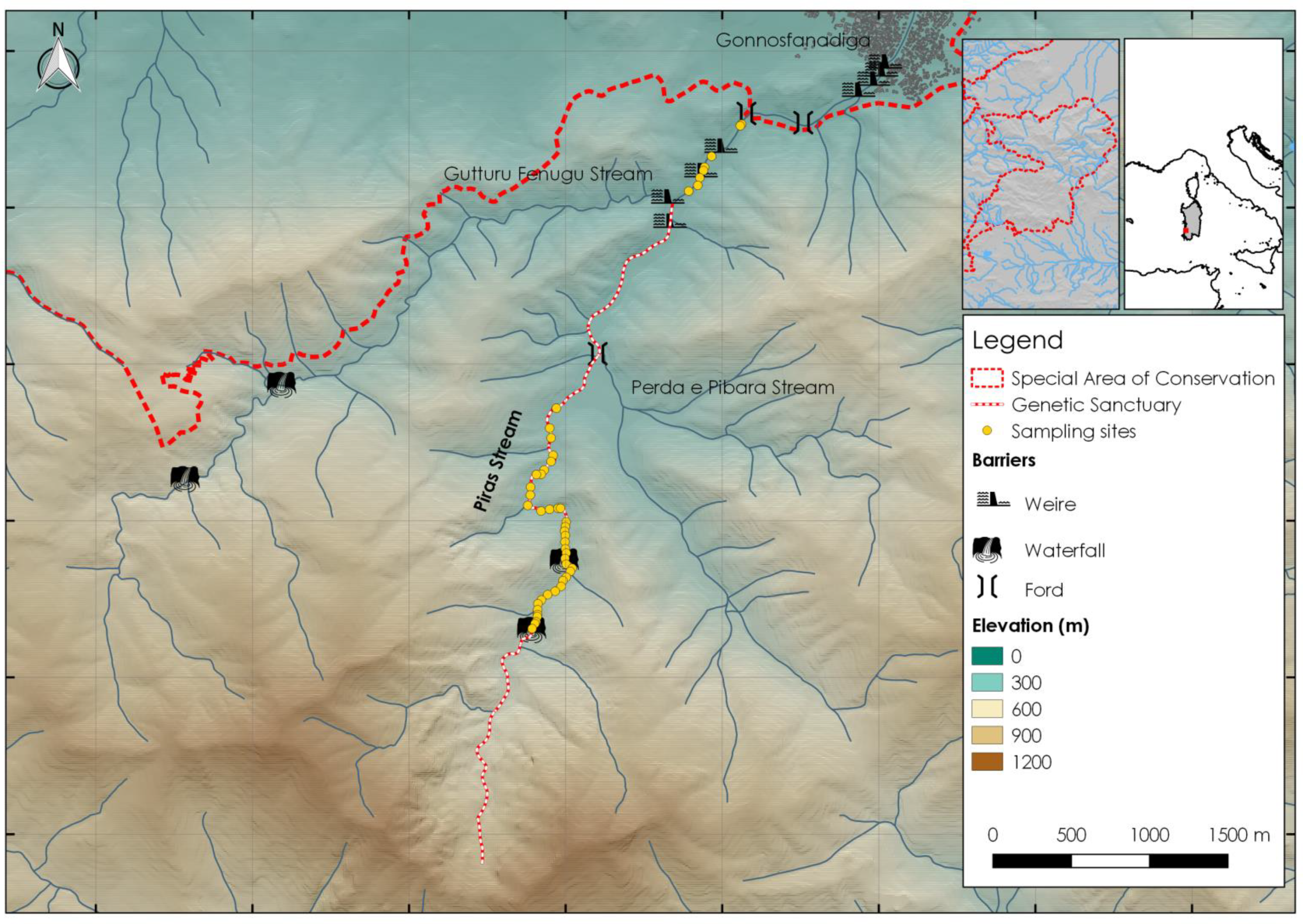
2.1. Study Area
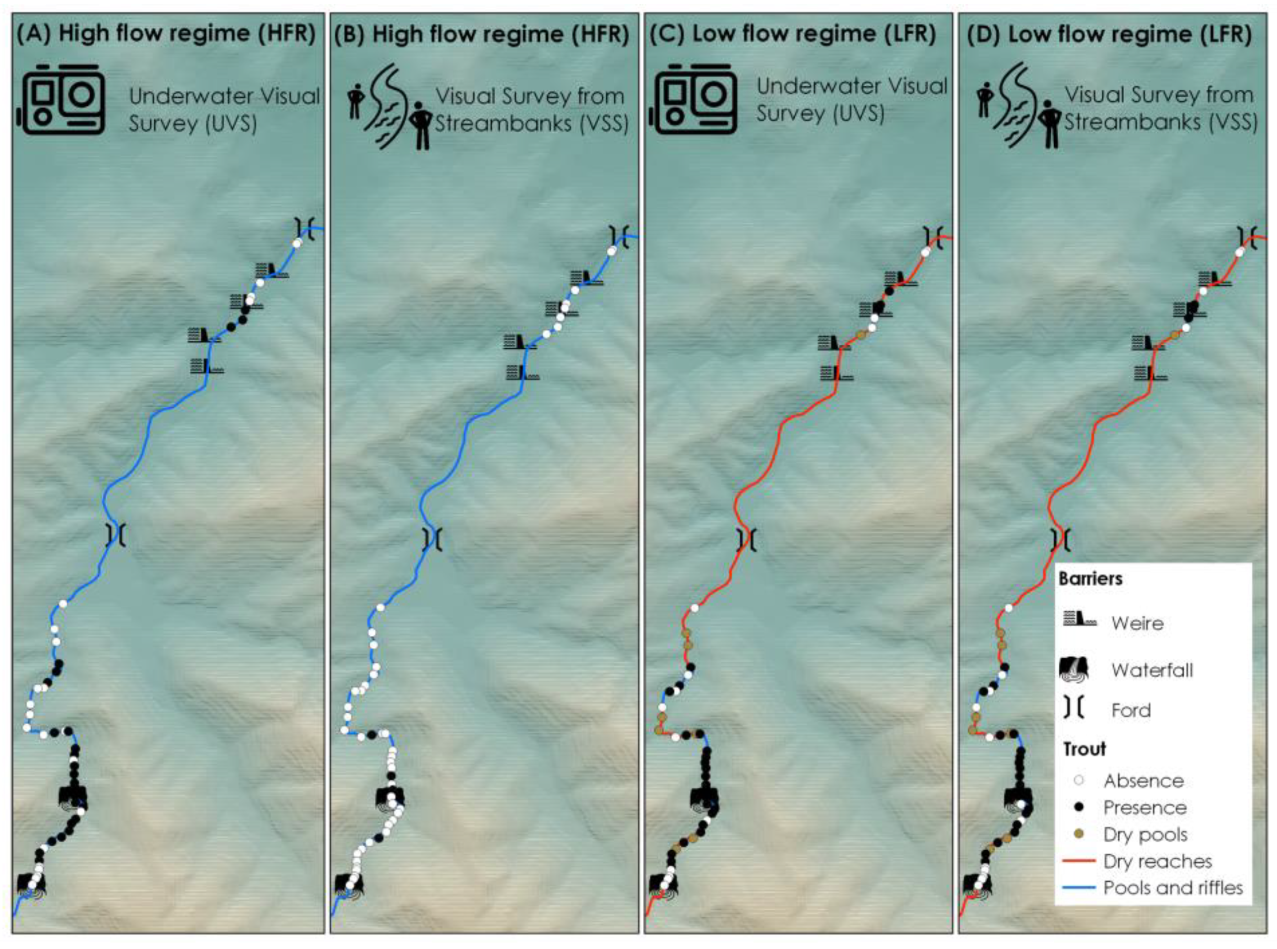
2.2. Data Collection
2.3. Environmental Variables
2.4. Data Analyses
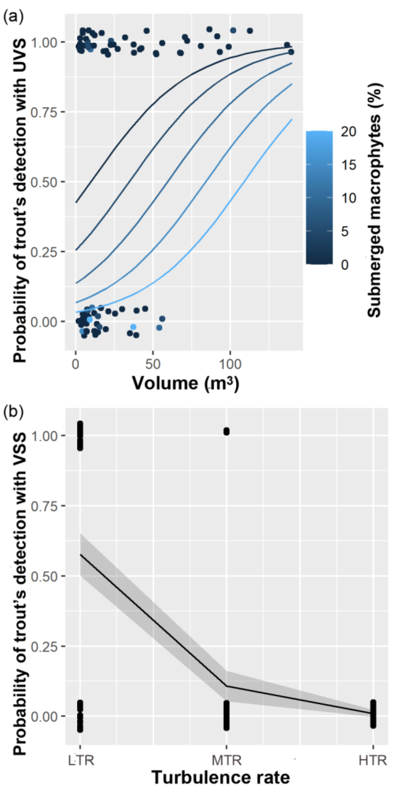
3. Results
4. Discussion
5. Conclusions
Supplementary Materials
Author Contributions
Funding
Institutional Review Board Statement
Informed Consent Statement
Data Availability Statement
Acknowledgments
Conflicts of Interest
References
- Maitland, P.S. The Conservation of Freshwater Fish: Past and Present Experience. Biol. Conserv. 1995, 72, 259–270. [Google Scholar] [CrossRef]
- Schmutz, S.; Cowx, I.G.; Haidvogl, G.; Pont, D. Fish-Based Methods for Assessing European Running Waters: A Synthesis. Fish. Manag. Ecol. 2007, 14, 369–380. [Google Scholar] [CrossRef]
- Aparicio, E.; Carmona-Catot, G.; Moyle, P.B.; García-Berthou, E. Development and Evaluation of a Fish-Based Index to Assess Biological Integrity of Mediterranean Streams. Aquat. Conserv. Mar. Freshw. Ecosyst. 2011, 21, 324–337. [Google Scholar] [CrossRef]
- Miranda, L.E.; Killgore, K.J. Abundance–Occupancy Patterns in a Riverine Fish Assemblage. Freshw. Biol. 2019, 64, 2221–2233. [Google Scholar] [CrossRef]
- Radinger, J.; Britton, J.R.; Carlson, S.M.; Magurran, A.E.; Alcaraz-Hernández, J.D.; Almodóvar, A.; Benejam, L.; Fernández-Delgado, C.; Nicola, G.G.; Oliva-Paterna, F.J.; et al. Effective Monitoring of Freshwater Fish. Fish Fish. 2019, 20, 729–747. [Google Scholar] [CrossRef] [Green Version]
- Lockwood, R.N.; Schneider, J.C. Stream Fish Population Estimates by Mark-and-Recapture and Depletion Methods. In Manual of Fisheries Survey Methods II: With Periodic Updates; University of Michigan: Ann Arbor, MI, USA, 2000; pp. 1–14. [Google Scholar]
- Zippin, C. An Evaluation of the Remevol Method of Estimating Animal Populations. Biometrics 1956, 12, 163–168. [Google Scholar] [CrossRef]
- Saunders, W.C.; Fausch, K.D.; White, G.C. Accurate Estimation of Salmonid Abundance in Small Streams Using Nighttime Removal Electrofishing: An Evaluation Using Marked Fish. N. Am. J. Fish. Manag. 2011, 31, 403–415. [Google Scholar] [CrossRef]
- Nielsen, J.L. Scientific Sampling Effects: Electrofishing California’s Endangered Fish Populations. Fisheries 1998, 23, 6–12. [Google Scholar] [CrossRef]
- Snyder, D.E. Invited Overview: Conclusions from a Review of Electrofishing and Its Harmful Effects on Fish. Rev. Fish Biol. Fish. 2004, 13, 445–453. [Google Scholar] [CrossRef]
- Dalbey, S.R.; McMahon, T.E.; Fredenberg, W. Effect of Electrofishing Pulse Shape and Electrofishing-Induced Spinal Injury on Long-Term Growth and Survival of Wild Rainbow Trout. N. Am. J. Fish. Manag. 1996, 16, 560–569. [Google Scholar] [CrossRef]
- Dolan, C.R.; Miranda, L.E. Injury and Mortality of Warmwater Fishes Immobilized by Electrofishing. N. Am. J. Fish. Manag. 2004, 24, 118–127. [Google Scholar] [CrossRef]
- Bennett, R.H.; Ellender, B.R.; Mäkinen, T.; Miya, T.; Pattrick, P.; Wasserman, R.J.; Woodford, D.J.; Weyl, O.L.F. Ethical Considerations for Field Research on Fishes. KOEDOE-African Prot. Area Conserv. Sci. 2016, 58, 77–90. [Google Scholar] [CrossRef] [Green Version]
- Costello, M.J.; Beard, K.H.; Corlett, R.T.; Cumming, G.S.; Devictor, V.; Loyola, R.; Maas, B.; Miller-Rushing, A.J.; Pakeman, R.; Primack, R.B. Field Work Ethics in Biological Research. Biol. Conserv. 2016, 203, 268–271. [Google Scholar] [CrossRef]
- Thurow, R.F.; Dolloff, C.A.; Marsden, J.E. Visual Observation of Fishes and Aquatic Habitat. In Fisheries Techniques; American Fisheries Society: Bethesda, MD, USA, 2013; p. 38. [Google Scholar]
- Ebner, B.C.; Starrs, D.; Morgan, D.L.; Fulton, C.J.; Donaldson, J.A.; Sean Doody, J.; Cousins, S.; Kennard, M.; Butler, G.; Tonkin, Z.; et al. Emergence of Field-Based Underwater Video for Understanding the Ecology of Freshwater Fishes and Crustaceans in Australia. J. R. Soc. West. Aust. 2014, 97, 287–296. [Google Scholar]
- Carim, K.J.; Wilcox, T.M.; Anderson, M.; Lawrence, D.J.; Young, M.K.; McKelvey, K.S.; Schwartz, M.K. An Environmental DNA Marker for Detecting Nonnative Brown Trout (Salmo trutta). Conserv. Genet. Resour. 2016, 8, 259–261. [Google Scholar] [CrossRef]
- Schumer, G.; Crowley, K.; Maltz, E.; Johnston, M.; Anders, P.; Blankenship, S. Utilizing Environmental DNA for Fish Eradication Effectiveness Monitoring in Streams. Biol. Invasions 2019, 21, 3415–3426. [Google Scholar] [CrossRef] [Green Version]
- Sepulveda, A.J.; Al-Chokhachy, R.; Laramie, M.B.; Crapster, K.; Knotek, L.; Miller, B.; Zale, A.V.; Pilliod, D.S. It’s Complicated. Environmental Dna as a Predictor of Trout and Char Abundance in Streams. Can. J. Fish. Aquat. Sci. 2021, 78, 422–432. [Google Scholar] [CrossRef]
- Wilson, K.; Allen, M.; Ahrens, R.; Netherland, M. Use of Underwater Video to Assess Freshwater Fish Populations in Dense Submersed Aquatic Vegetation. Mar. Freshw. Res. 2014, 66, 10–22. [Google Scholar] [CrossRef] [Green Version]
- Jordan, F.; Jelks, H.L.; Bortone, S.A.; Dorazio, R.M. Comparison of Visual Survey and Seining Methods for Estimating Abundance of an Endangered, Benthic Stream Fish. Environ. Biol. Fishes 2008, 81, 313–319. [Google Scholar] [CrossRef]
- Castañeda, R.A.; Van Nynatten, A.; Crookes, S.; Ellender, B.R.; Heath, D.D.; MacIsaac, H.J.; Mandrak, N.E.; Weyl, O.L.F. Detecting Native Freshwater Fishes Using Novel Non-Invasive Methods. Front. Environ. Sci. 2020, 8, 29. [Google Scholar] [CrossRef]
- Westhoff, J.T.; Berkman, L.K.; Klymus, K.E.; Thompson, N.L.; Richter, C.A. A Comparison of EDNA and Visual Survey Methods for Detection of Longnose Darter Percina Nasuta in Missouri. Fishes 2022, 7, 70. [Google Scholar] [CrossRef]
- Chamberland, J.M.; Lanthier, G.; Boisclair, D. Comparison between Electrofishing and Snorkeling Surveys to Describe Fish Assemblages in Laurentian Streams. Environ. Monit. Assess. 2014, 186, 1837–1846. [Google Scholar] [CrossRef] [PubMed]
- Joyce, M.P.; Hubert, W.A. Snorkeling as an Alternative to Deplation Eletrofishing for Assessing Cutthroat Trout and Brown Trout in Stream Pools. J. Freshw. Ecol. 2003, 18, 215–222. [Google Scholar] [CrossRef]
- Albanese, B.; Owers, K.A.; Weiler, D.A.; Pruitt, W. Estimating Occupancy of Rare Fishes Using Visual Surveys, with a Comparison to Backpack Electrofishing. Southeast. Nat. 2011, 10, 423–442. [Google Scholar] [CrossRef]
- Ellender, B.R.; Becker, A.; Weyl, O.L.F.; Swartz, E.R. Underwater Video Analysis as a Non-Destructive Alternative to Electrofishing for Sampling Imperilled Headwater Stream Fishes. Aquat. Conserv. Mar. Freshw. Ecosyst. 2012, 22, 58–65. [Google Scholar] [CrossRef]
- Castañeda, R.A.; Weyl, O.L.F.; Mandrak, N.E. Using Occupancy Models to Assess the Effectiveness of Underwater Cameras to Detect Rare Stream Fishes. Aquat. Conserv. Mar. Freshw. Ecosyst. 2020, 30, 565–576. [Google Scholar] [CrossRef]
- Hannweg, B.; Marr, S.M.; Bloy, L.E.; Weyl, O.L.F. Using Action Cameras to Estimate the Abundance and Habitat Use of Threatened Fish in Clear Headwater Streams. African J. Aquat. Sci. 2020, 45, 372–377. [Google Scholar] [CrossRef]
- Ebner, B.C.; Morgan, D.L. Using Remote Underwater Video to Estimate Freshwater Fish Species Richness. J. Fish Biol. 2013, 82, 1592–1612. [Google Scholar] [CrossRef]
- Bozek, M.A.; Rahel, F.J. Comparison of Streamside Visual Counts to Electrofishing Estimates of Colorado River Cutthroat Trout Fry and Adults. N. Am. J. Fish. Manag. 1991, 11, 38–42. [Google Scholar] [CrossRef]
- Lambert, T.R.; Hanson, D.F. Development of Habitat Suitability Criteria for Trout in Small Streams. Regul. Rivers Res. Manag. 1989, 3, 291–303. [Google Scholar] [CrossRef]
- Brewer, S.K.; Ellersieck, M.R. Evaluating Two Observational Sampling Techniques for Determining the Distribution and Detection Probability of Age-0 Smallmouth Bass in Clear, Warmwater Streams. N. Am. J. Fish. Manag. 2011, 31, 894–904. [Google Scholar] [CrossRef]
- King, A.J.; George, A.; Buckle, D.J.; Novak, P.A.; Fulton, C.J. Efficacy of Remote Underwater Video Cameras for Monitoring Tropical Wetland Fishes. Hydrobiologia 2018, 807, 145–164. [Google Scholar] [CrossRef]
- Castañeda, R.A.; Mandrak, N.E.; Barrow, S.; Weyl, O.L.F. Occupancy Dynamics of Rare Cyprinids after Invasive Fish Eradication. Aquat. Conserv. Mar. Freshw. Ecosyst. 2020, 30, 1424–1436. [Google Scholar] [CrossRef]
- Fernández, M.V.; Macchi, P.J.; Sosnovsky, A.; Zattara, E.E.; Lallement, M.E.; Milano, D. Spawning Aggregation Behaviour in the Creole Perch, Percichthys trucha (Percichthyidae): A Target Species for Conservation. Aquat. Conserv. Mar. Freshw. Ecosyst. 2021, 31, 3248–3260. [Google Scholar] [CrossRef]
- Kottelat, M.; Freyhof, J. Handbook of European Freshwater Fishes; Kottelat, M., Freyhof, J., Eds.; Springer: Berlin, Germany, 2007. [Google Scholar]
- Splendiani, A.; Palmas, F.; Sabatini, A.; Barucchi, V.C. The Name of the Trout: Considerations on the Taxonomic Status of the Salmo trutta L., 1758 Complex (Osteichthyes: Salmonidae) in Italy. Eur. Zool. J. 2019, 86, 432–442. [Google Scholar] [CrossRef] [Green Version]
- Tougard, C. Will the Genomics Revolution Finally Solve the Salmo Systematics? Hydrobiologia 2022, 849, 2209–2224. [Google Scholar] [CrossRef]
- Tougard, C.; Justy, F.; Guinand, B.; Douzery, E.J.P.; Berrebi, P. Salmo macrostigma (Teleostei, Salmonidae): Nothing More than a Brown Trout (S. trutta) Lineage? J. Fish Biol. 2018, 93, 302–310. [Google Scholar] [CrossRef] [Green Version]
- Polgar, G.; Iaia, M.; Righi, T.; Volta, P. The Italian Alpine and Subalpine Trouts: Taxonomy, Evolution, and Conservation. Biology 2022, 11, 576. [Google Scholar] [CrossRef]
- Hashemzadeh Segherloo, I.; Freyhof, J.; Berrebi, P.; Ferchaud, A.L.; Geiger, M.; Laroche, J.; Levin, B.A.; Normandeau, E.; Bernatchez, L. A Genomic Perspective on an Old Question: Salmo Trouts or Salmo trutta (Teleostei: Salmonidae)? Mol. Phylogenet. Evol. 2021, 162, 107204. [Google Scholar] [CrossRef]
- Rondinini, C.; Battistoni, A.; Teofili, C. Lista Rossa IUCN Dei Vertebrati Italiani 2022; Comitato Italiano IUCN e Ministero Dell’Ambiente e Della Sicurezza Energetica: Roma, Italy, 2022. [Google Scholar]
- Clavero, M.; Hermoso, V.; Levin, N.; Kark, S. Geographical Linkages between Threats and Imperilment in Freshwater Fish in the Mediterranean Basin. Divers. Distrib. 2010, 16, 744–754. [Google Scholar] [CrossRef]
- Ayllón, D.; Almodóvar, A.; Nicola, G.G.; Parra, I.; Elvira, B. A New Biological Indicator to Assess the Ecological Status of Mediterranean Trout Type Streams. Ecol. Indic. 2012, 20, 295–303. [Google Scholar] [CrossRef]
- Splendiani, A.; Giovannotti, M.; Righi, T.; Fioravanti, T.; Cerioni, P.N.; Lorenzoni, M.; Carosi, A.; La Porta, G.; Barucchi, V.C. Introgression despite Protection: The Case of Native Brown Trout in Natura 2000 Network in Italy. Conserv. Genet. 2019, 20, 343–356. [Google Scholar] [CrossRef]
- Gratton, P.; Allegrucci, G.; Sbordoni, V.; Gandolfi, A. The Evolutionary Jigsaw Puzzle of the Surviving Trout (Salmo trutta L. Complex) Diversity in the Italian Regionion a Multilocus Bayesian Approach. Mol. Phylogenet. Evol. 2014, 79, 292–304. [Google Scholar] [CrossRef] [PubMed]
- Rossi, A.; Talarico, L.; Petrosino, L.; Crescenzo, S.; Tancioni, L. Conservation Genetics of Mediterranean Brown Trout in Central Italy (Latium): A Multi-Marker Approach. Water 2022, 14, 937. [Google Scholar] [CrossRef]
- Berrebi, P.; Caputo Barucchi, V.; Splendiani, A.; Muracciole, S.; Sabatini, A.; Palmas, F.; Tougard, C.; Arculeo, M.; Marić, S. Brown Trout (Salmo trutta L.) High Genetic Diversity around the Tyrrhenian Sea as Revealed by Nuclear and Mitochondrial Markers. Hydrobiologia 2019, 826, 209–231. [Google Scholar] [CrossRef]
- Almodóvar, A.; Nicola, G.G.; Ayllón, D.; Elvira, B. Global Warming Threatens the Persistence of Mediterranean Brown Trout. Glob. Chang. Biol. 2012, 18, 1549–1560. [Google Scholar] [CrossRef] [Green Version]
- Ayllón, D.; Railsback, S.F.; Harvey, B.C.; García, I.; Nicola, G.G.; Elvira, B.; Almodóvar, A. Mechanistic Simulations Predict That Thermal and Hydrological Effects of Climate Change on Mediterranean Trout Cannot Be Offset by Adaptive Behaviour, Evolution, and Increased Food Production. Sci. Total Environ. 2019, 693, 133648. [Google Scholar] [CrossRef]
- Lorenzoni, M.; Carosi, A.; Giovannotti, M.; Porta, G.L.; Barucchi, V.C. Population Status of the Native Cottus gobio after Removal of the Alien Salmo trutta: A Case-Study in Two Mediterranean Streams. Knowl. Manag. Aquat. Ecosyst 2018, 419, 22. [Google Scholar] [CrossRef] [Green Version]
- Carosi, A.; Ghetti, L.; Padula, R.; Lorenzoni, M. Population Status and Ecology of the Salmo trutta Complex in an Italian River Basin under Multiple Anthropogenic Pressures. Ecol. Evol. 2020, 10, 7320–7333. [Google Scholar] [CrossRef]
- Zaccara, S.; Trasforini, S.; Antognazza, C.M.; Puzzi, C.; Britton, J.R.; Crosa, G. Morphological and Genetic Characterization of Sardinian Trout Salmo cettii Rafinesque, 1810 and Their Conservation Implications. Hydrobiologia 2015, 760, 205–223. [Google Scholar] [CrossRef]
- Sabatini, A.; Cannas, R.; Follesa, M.C.; Palmas, F.; Manunza, A.; Matta, G.; Pendugiu, A.A.; Serra, P.; Cau, A. Genetic Characterization and Artificial Reproduction Attempt of Endemic Sardinian Trout Salmo trutta L., 1758 (Osteichthyes, Salmonidae): Experiences in Captivity. Ital. J. Zool. 2011, 78, 20–26. [Google Scholar] [CrossRef]
- Sabatini, A.; Podda, C.; Frau, G.; Cani, M.V.; Musu, A.; Serra, M.; Palmas, F. Restoration of Native Mediterranean Brown Trout Salmo cettii Rafinesque, 1810 (Actinopterygii: Salmonidae) Populations Using an Electric Barrier as a Mitigation Tool. Eur. Zool. J. 2018, 85, 138–150. [Google Scholar] [CrossRef] [Green Version]
- Berrebi, P. Three Brown Trout Salmo trutta Lineages in Corsica Described through Allozyme Variation. J. Fish Biol. 2015, 86, 60–73. [Google Scholar] [CrossRef] [PubMed]
- Palmas, F.; Righi, T.; Musu, A.; Frongia, C.; Podda, C.; Serra, M.; Splendiani, A.; Caputo Barucchi, V.; Sabatini, A. Pug-Headedness Anomaly in a Wild and Isolated Population of Native Mediterranean Trout Salmo trutta L., 1758 Complex (Osteichthyes: Salmonidae ). Diversity 2020, 12, 353. [Google Scholar] [CrossRef]
- Berrebi, P.; Povz, M.; Jesensek, D.; Cattaneo-Berrebi, G.; Crivelli, A.J. The Genetic Diversity of Native, Stocked and Hybrid Populations of Marble Trout in the Soca River, Slovenia. Heredity 2000, 85, 277–287. [Google Scholar] [CrossRef]
- Sato, T.; Harada, Y. Loss of Genetic Variation and Effective Population Size of Kirikuchi Charr: Implications for the Management of Small, Isolated Salmonid Populations. Anim. Conserv. 2008, 11, 153–159. [Google Scholar] [CrossRef]
- Vincenzi, S.; Crivelli, A.J.; Jesenšek, D.; De Leo, G.A. The Management of Small, Isolated Salmonid Populations: Do We Have to Fix It If It Ain’t Broken? Anim. Conserv. 2010, 13, 21–23. [Google Scholar] [CrossRef]
- Stubbington, R.; Chadd, R.; Cid, N.; Csabai, Z.; Miliša, M.; Morais, M.; Munné, A.; Pařil, P.; Pešić, V.; Tziortzis, I.; et al. Biomonitoring of Intermittent Rivers and Ephemeral Streams in Europe: Current Practice and Priorities to Enhance Ecological Status Assessments. Sci. Total Environ. 2018, 618, 1096–1113. [Google Scholar] [CrossRef]
- Poteaux, C.; Berrebi, P. Intégrité Génomique et Repeuplements Chez La Truite Commune Du Versant Méditerranéen. Bull. Fr. Pêche Piscic. 1997, 344–345, 309–322. [Google Scholar] [CrossRef] [Green Version]
- Podda, C.; Palmas, F.; Pusceddu, A.; Sabatini, A. When the Eel Meets Dams: Larger Dams’ Long-Term Impacts on Anguilla anguilla (L., 1758). Front. Environ. Sci. 2022, 10, 876369. [Google Scholar] [CrossRef]
- Naselli-Flores, L.; Lugliè, A.; Naselli-flores, L.; Lugliè, A. Laghi Artificiali Dell’ Italia Meridionale e Delle Isole Maggiori. Biol. Ambient. 2014, 28, 41–48. [Google Scholar]
- Palmas, F.; Cau, A.; Podda, C.; Musu, A.; Serra, M.; Pusceddu, A.; Sabatini, A. Rivers of Waste: Anthropogenic Litter in Intermittent Sardinian Rivers, Italy (Central Mediterranean). Environ. Pollut. 2022, 302, 119073. [Google Scholar] [CrossRef] [PubMed]
- Ayllón, D.; Almodóvar, A.; Nicola, G.G.; Elvira, B. Ontogenetic and Spatial Variations in Brown Trout Habitat Selection. Ecol. Freshw. Fish 2010, 19, 420–432. [Google Scholar] [CrossRef]
- Armstrong, J.D.; Kemp, P.S.; Kennedy, C.J.; Ladle, M.; Milner, N.J. Habitat Requirements of Atlantic Salmon and Brown Trout in Rivers and Streams. Fish. Res. 2003, 62, 143–170. [Google Scholar] [CrossRef]
- Platts, W.S.; Megahan, W.F.; Minshall, W.G. Methods for Evaluating Stream, Riparian, and Biotic Conditions; US Department of Agriculture, Forest Service, Intirmountain Forest and Range Experiment Station: Ogden, UT, USA, 1983. [Google Scholar]
- Hering, D.; Moog, O.; Sandin, L.; Verdonschot, P.F.M. Overview and Application of the AQEM Assessment System. Hydrobiologia 2004, 516, 1–20. [Google Scholar] [CrossRef]
- Ayllón, D.; Almodovar, A.; Nicola, G.; Elvira, B. Modelling Brown Trout Spatial Requirements through Physical Habitat Simulations. River Res. Appl. 2010, 26, 1090–1102. [Google Scholar] [CrossRef]
- Zuur, A.F.; Ieno, E.N.; Elphick, C.S. A Protocol for Data Exploration to Avoid Common Statistical Problems. Methods Ecol. Evol. 2010, 1, 3–14. [Google Scholar] [CrossRef]
- Burnham, K.P.; Anderson, D.R. Model Selection and Inference: A Practical Information-Theoretic Approach, 2nd ed.; Springer: New York, NY, USA, 2002; ISBN 0387953647. [Google Scholar]
- Calcagno, V.; de Mazancourt, C. Glmulti: An R Package for Easy Automated Model Selection with (Generalized) Linear Models. J. Stat. Softw. 2010, 34, 29. [Google Scholar] [CrossRef] [Green Version]
- Crawley, M.J. The R Book; John Wiley & Sons, Inc.: Hoboken, NJ, USA, 2013; ISBN 9780470973929. [Google Scholar]
- Larios-López, J.E.; Tierno de Figueroa, J.M.; Alonso-González, C.; Nebot Sanz, B. Distribution of Brown Trout (Salmo trutta Linnaeus, 1758) (Teleostei: Salmonidae) in Its Southwesternmost European Limit: Possible Causes. Ital. J. Zool. 2015, 82, 404–415. [Google Scholar] [CrossRef] [Green Version]
- Clavero, M.; Calzada, J.; Esquivias, J.; Veríssimo, A.; Hermoso, V.; Qninba, A.; Delibes, M. Nowhere to Swim to: Climate Change and Conservation of the Relict Dades Trout Salmo Multipunctata in the High Atlas Mountains, Morocco. Oryx 2018, 52, 627–635. [Google Scholar] [CrossRef]
- Struthers, D.P.; Danylchuk, A.J.; Wilson, A.D.M.; Cooke, S.J. Action Cameras: Bringing Aquatic and Fisheries Research into View. Fisheries 2015, 40, 504–512. [Google Scholar] [CrossRef] [Green Version]
- Colton, M.A.; Swearer, S.E. A Comparison of Two Survey Methods: Differences between Underwater Visual Census and Baited Remote Underwater Video. Mar. Ecol. Prog. Ser. 2010, 400, 19–36. [Google Scholar] [CrossRef] [Green Version]
- Elliott, J.M. Pools as Refugia for Brown Trout during Two Summer Droughts: Trout Responses to Thermal and Oxygen Stress. J. Fish Biol. 2000, 56, 938–948. [Google Scholar] [CrossRef]
- McKenzie, D.; Nichols, J.; Royle, J.; Pollock, K.; Bailey, L.; Hines, J. Occupancy Estimation and Modelling. Inferring Patterns and Dynamics of Species Occurence; Elsevier: San Diego, CA, USA, 2006. [Google Scholar]
- Bailey, L.L.; Simons, T.R.; Pollock, K.H. Estimating Site Occupancy and Species Detection Probability Parameters for Terrestrial Salamanders. Ecol. Appl. 2004, 14, 692–702. [Google Scholar] [CrossRef] [Green Version]
- Ayllón, D.; Almodovar, A.; Nicola, G.; Elvira, B. Interactive Effects of Cover and Hydraulics on Brown Trout Habitat Selection Patterns. River Res. Appl. 2009, 25, 1051–1065. [Google Scholar] [CrossRef]
- Vismara, R.; Azzellino, A.; Bosi, R.; Crosa, G.; Gentili, G. Habitat Suitability Curves for Brown Trout (Salmo trutta fario L.) in the River Adda, Northern Italy: Comparing Univariate and Multivariate Approaches. River Res. Appl. 2001, 17, 37–50. [Google Scholar] [CrossRef]
- Binder, T.R.; Thompson, H.T.; Muir, A.M.; Riley, S.C.; Marsden, J.E.; Bronte, C.R.; Krueger, C.C. New Insight into the Spawning Behavior of Lake Trout, Salvelinus namaycush, from a Recovering Population in the Laurentian Great Lakes. Environ. Biol. Fishes 2015, 98, 173–181. [Google Scholar] [CrossRef]


| Underwater Visual Survey (UVS) | |||||||||
| Rank | Model effect | Ka | AICc | ΔAICc | Dev. Expl. (%) | Slope | SE | p | LRT |
| 1 | Volume (m3) | 2 | 109.598 | 0 | 10.00% | 0.03 | 0.01 | 0.0042 ** | 0.0005 *** |
| 2 | Submerged_macrophyte (%) | 2 | 116.132 | 6.534081 | 4.72% | −0.15 | 0.07 | 0.0491 * | 0.01844 * |
| 3 | Boulder (%) | 2 | 116.274 | 6.675573 | 4.60% | −0.02 | 0.009 | 0.0233 * | 0.01999 * |
| 4 | Riparian_vegetation (%) | 2 | 118.789 | 9.190578 | 2.46% | 0.05 | 0.03 | 0.101 | |
| 5 | M0 | 1 | 119.589 | 9.990974 | |||||
| 6 | Green_Algae (%) | 2 | 121.541 | 11.94337 | |||||
| 7 | Roots (%) | 2 | 121.604 | 12.00592 | |||||
| 8 | Turbulence_rate (High, Medium, Low) | 2 | 121.67 | 12.07229 | |||||
| 9 | Turbidity (NTU) | 2 | 121.685 | 12.08668 | |||||
| Visual Survey from Streambanks (VSS) | |||||||||
| Rank | Model effect | Ka | AICc | ΔAICc | Dev. Expl. (%) | Slope | SE | p | LRT |
| 1 | Turbulence_rate (High, Medium, Low) | 2 | 80.1 | 0 | 29.03% | −2.42 | 0.62 | 0.0001 *** | 2.4 × 10⁸ *** |
| 2 | Turbidity (NTU) | 2 | 100.34 | 20.24 | 10.11% | 2.19 | 0.7 | 0.0018 ** | 0.0009977 *** |
| 3 | Boulder (%) | 2 | 107.16 | 27.07 | 3.73% | −0.02 | 0.01 | 0.0555 | 0.0455 * |
| 4 | Riparian_vegetation (%) | 2 | 108.21 | 28.11 | 2.75% | 0.06 | 0.03 | 0.087 | |
| 5 | Submerged_macrophyte (%) | 2 | 108.58 | 28.48 | 2.41% | −0.12 | 0.09 | 0.192 | |
| 6 | M0 | 1 | 109.07 | 28.29 | |||||
| 7 | Roots (%) | 2 | |||||||
| 8 | Volume (m3) | 2 | |||||||
| 9 | Green_Algae (%) | 2 | |||||||
| Underwater Visual Survey (UVS) | ||||
| Rank | Model Decription | AICc | ΔAICc | Weights (wi) |
| 1 | UVS ~ 1 + Volume + Submerged_Macrophytes | 106.70 | 0.00 | 0.47 |
| 2 | UVS ~ 1 + Volume + Boulder + Submerged_Macrophytes | 107.54 | 0.83 | 0.31 |
| 3 | UVS ~ 1 + Volume | 109.60 | 2.90 | 0.11 |
| 4 | UVS ~ 1 + Volume + Boulder | 110.76 | 4.06 | 0.06 |
| 5 | UVS ~ 1 + Boulder + Submerged_Macrophytes | 112.14 | 5.44 | 0.03 |
| 6 | UVS ~ 1 + Submerged_Macrophytes | 116.13 | 9.43 | 0.00 |
| 7 | UVS ~ 1 + Boulder | 116.27 | 9.57 | 0.00 |
| 8 | UVS ~ 1 | 119.59 | 12.89 | 0.00 |
| Visual Survey from Streambanks (VSS) | ||||
| Rank | Model Decription | AICc | ΔAICc | Weights (wi) |
| 1 | VSS ~ 1 + Turbulence_rate + Boulder | 79.16 | 0.00 | 0.43 |
| 2 | VSS ~ 1 + Turbulence_rate | 80.10 | 0.93 | 0.27 |
| 3 | VSS ~ 1 + Turbulence_rate + Turbidity + Boulder | 80.64 | 1.48 | 0.20 |
| 4 | VSS ~ 1 + Turbulence_rate + Turbidity | 82.03 | 2.87 | 0.10 |
| 5 | VSS ~ 1 + Turbidity + Boulder | 99.75 | 20.59 | 0. 01 |
| 6 | VSS ~ 1 + Turbidity | 100.34 | 21.17 | 0.01 |
| 7 | VSS ~ 1 + Boulder | 107.17 | 28.01 | 0.00 |
| 8 | VSS ~ 1 | 1109.07 | 1029.91 | 0.00 |
| Underwater Visual Survey (UVS) | |||
|---|---|---|---|
| Effect | Estimate | Unconditional Variance | Importance |
| Boulder | −0.0053 | 7.37 × 10⁵ | 0.4097 |
| Submerged_Macrophytes | −0.1279 | 8.82 × 10³ | 0.8216 |
| Volume | 0.0278 | 1.49 × 10⁴ | 0.9598 |
| Visual Survey from Streambanks (VSS) | |||
| Turbidity | −0.2200 | 0.2480 | 0.3054 |
| Boulder | −0.0136 | 0.0002 | 0.6305 |
| Turbulence rate | −2.5892 | 0.5194 | 0.9999 |
Disclaimer/Publisher’s Note: The statements, opinions and data contained in all publications are solely those of the individual author(s) and contributor(s) and not of MDPI and/or the editor(s). MDPI and/or the editor(s) disclaim responsibility for any injury to people or property resulting from any ideas, methods, instructions or products referred to in the content. |
© 2023 by the authors. Licensee MDPI, Basel, Switzerland. This article is an open access article distributed under the terms and conditions of the Creative Commons Attribution (CC BY) license (https://creativecommons.org/licenses/by/4.0/).
Share and Cite
Palmas, F.; Casula, P.; Curreli, F.; Podda, C.; Cabiddu, S.; Sabatini, A. Exploring Less Invasive Visual Surveys to Assess the Spatial Distribution of Endangered Mediterranean Trout Population in a Small Intermittent Stream. Biology 2023, 12, 1000. https://doi.org/10.3390/biology12071000
Palmas F, Casula P, Curreli F, Podda C, Cabiddu S, Sabatini A. Exploring Less Invasive Visual Surveys to Assess the Spatial Distribution of Endangered Mediterranean Trout Population in a Small Intermittent Stream. Biology. 2023; 12(7):1000. https://doi.org/10.3390/biology12071000
Chicago/Turabian StylePalmas, Francesco, Paolo Casula, Francesco Curreli, Cinzia Podda, Serenella Cabiddu, and Andrea Sabatini. 2023. "Exploring Less Invasive Visual Surveys to Assess the Spatial Distribution of Endangered Mediterranean Trout Population in a Small Intermittent Stream" Biology 12, no. 7: 1000. https://doi.org/10.3390/biology12071000