1. Introduction
Circular RNA (circRNA) is a special kind of single-stranded circular endogenous non-coding RNA (ncRNA). Recent research shows that endogenous circRNAs are widely distributed in mammalian cells and involved in transcriptional and posttranscriptional gene expression regulation [
1]. CircRNA was first discovered in RNA viruses as early as 1976 [
2], and in 1979, Hsu et al. provided electron microscopic evidence for the circular form of RNA [
3]. Over the following three decades, only a handful of circRNAs were discovered by chance [
4,
5,
6], and due to their low levels of expression, circRNAs were typically considered to be products of “noise” of an abnormal RNA splicing process, which resulted in circRNAs not receiving corresponding attention.
However, since 2010, with the development of RNA-seq technologies and specialized computational pipelines, many circRNAs have been widely recognized and discovered in eukaryotes, such as mice [
7], archaea [
8], and humans [
9]. With the progress in circRNA research, many circRNAs have been proven to present tissue-specific expression patterns and have specific biological functions [
10]. Emerging experimental results show that endogenous circRNAs widely exist in mammals and can work as miRNA sponges, which means that circRNAs reverse the inhibitory effect of the miRNA on its target gene and consequently repress their function [
11]. At present, many types of research have indicated the association between miRNA sponges (circRNAs) and human diseases.
CircRNAs have a prominent role in cancer diagnosis and treatment [
12]. For example, in bladder cancer studies, circ-ITCH acted as a miRNA sponge to inhibit bladder cancer progression by directly regulating p21 and PTEN in combination with miR-17 and miR-224. Circ-ITCH expression was also lower than normal in bladder cancer tissues [
13]. In addition, high expression of another circRNA, circ-TFRC, was detected in bladder cancer patients, which means that circ-TFRC promotes bladder cancer progression by binding to miR-107 [
14]. CircCCDC9 expression was significantly lower than normal in gastric cancer tissue samples, and the study confirmed that circCCDC9 inhibits the progression of gastric cancer by regulating CAV1 in combination with miR-6729-3p [
15]. CircRNA also plays an important role in the development of renal cell carcinoma (RCC) by regulating CDKN3/E2F1 in combination with miR-127-3p [
16]. These results suggest that investigating circRNA–miRNA interactions could be key to diagnosing and addressing complex diseases such as cancer.
Compared with traditional biological experimental methods, which are limited to small scales and require lots of labor and time, using computational models to predict the association between molecules can provide the basis for biological experiments at a low cost. At present, many computational methods have been proposed and applied to predict the correlation between different molecules. For example, Wang et al. proposed a model, SAEMDA, through a new unsupervised training method named Stacked Autoencoder to predict miRNA–disease associations [
17]. Ren et al. developed a model named BioChemDDI, which combines a Natural Language Processing algorithm and Hierarchical Representation Learning to effectively extract information, employed Similarity Network Fusion to fuse multiple features, and finally applied a deep neural network to obtain the predicted results [
18]. Wang et al. proposed a new method that extracts deep features of molecular similarity through a deep convolutional neural network and sends them to an extreme learning machine classifier to identify potential circRNA–miRNA associations [
19]. Such computational methods have achieved gratifying results and provided an experimental basis for further wet experiments.
Compared with related fields, where new circRNA molecules are constantly discovered and the nomenclature is not fully standardized, there are a few computational methods that predict associations between circRNAs and miRNAs. However, with the rapid development of high-throughput sequencing technology, a large number of databases have been developed to store circRNA-related information, such as circR2Disease [
20], circRNAdisease [
21], circbank [
22], and circBase [
23]. The circR2Disease database is a high-quality database containing detailed information about circRNA. The latest version contains about 750 circRNA–disease associations between more than 600 circRNAs and 100 diseases. The circRNAdisease database manually collects verified circRNA–disease pairs from the PubMed database by retrieving circRNA and disease keywords. Circbank is a comprehensive database that contains multiple characteristics of circRNA; more than 140,000 circRNAs from different sources can be retrieved by users from the circbank database. The circBase database is one of the early databases to collect circRNA information, including circRNA data, evidence to support circRNA expression, and scripts for identifying known and new circRNAs in sequencing data. The establishment of these databases has provided the materials for predicting associations between circRNAs and miRNAs by using computational methods.
At present, only few models have been proposed, and the predicted results were confirmed in PubMed. Compared with other fields, there are few computational prediction models for circRNA–miRNA interaction prediction. Therefore, it is urgent to develop new and effective prediction methods for circRNA–miRNA association prediction.
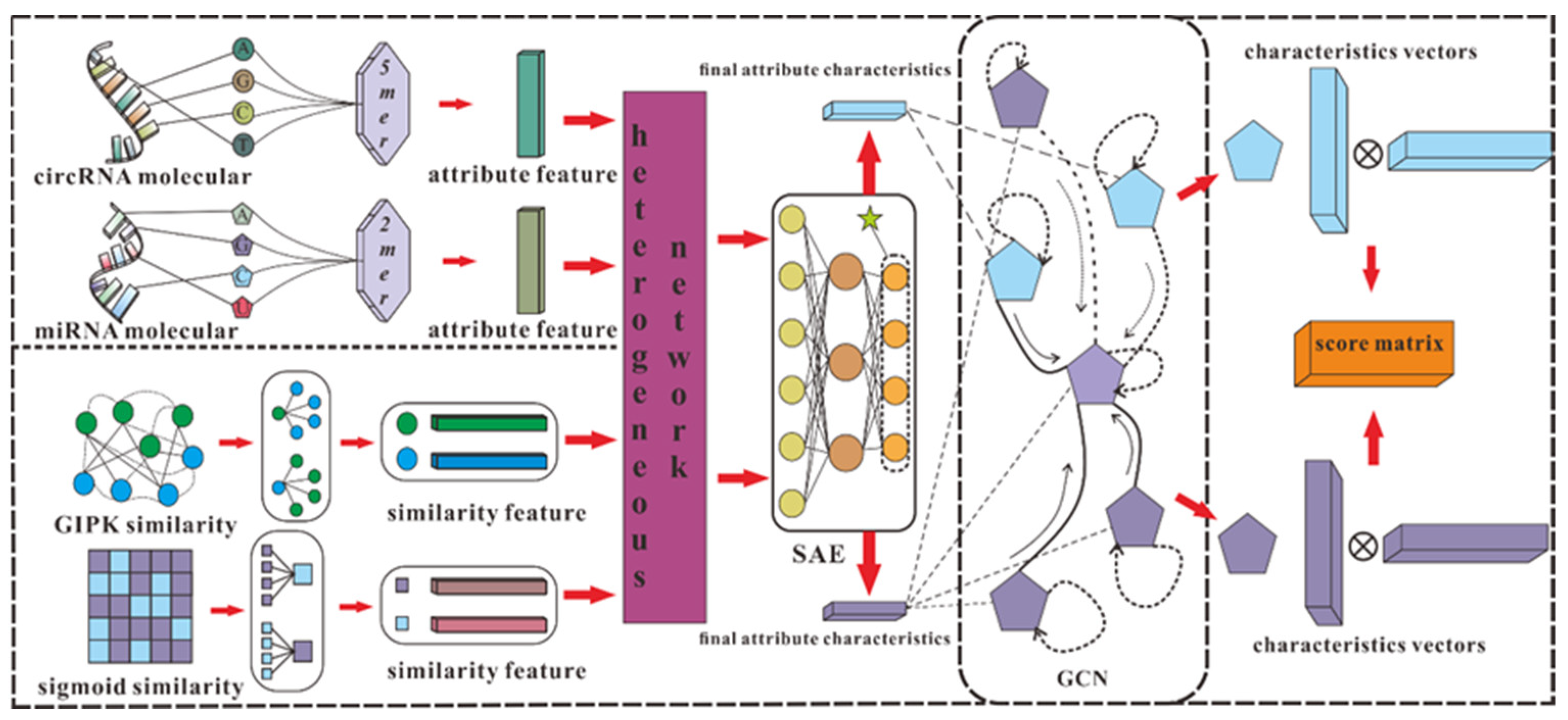
According to our understanding, there are some obstacles to using computational methods to predict circRNA–miRNA interactions: (i) The length of circRNA and miRNA sequences varies greatly, resulting in redundancy or sparsity of biological information collected. (ii) A network composed of confirmed circRNA–miRNA associations is difficult to connect, which means it is difficult to extract effective features from relatively isolated nodes. (iii) The data on circRNA–miRNA interactions are scattered among different databases, so it is difficult to collect comprehensive and reliable data. To solve these problems, we developed a model, SGCNCMI, to predict circRNA–miRNA interactions based on multi-source feature extraction and graph representation learning with a layer contribution mechanism. Specifically, we first adopt a K-mer algorithm to extract the internal attribute features in the sequence by taking the most appropriate K value for different RNAs, and to make full use of RNA molecular biological information, two kinds of kernel functions are added to enrich semantic descriptors. Secondly, we introduce the Sparse Autoencoder (SAE) with a sparsity penalty term to process semantic descriptors to obtain the most valuable molecular biological attribute information. Next, we apply a multilayer graph convolutional neural network (GCN) to project the circRNA–miRNA interaction network into a new space to capture non-linear interactions and hidden associations. Meanwhile, we include a layer contribution mechanism in the graph convolutional layer to ensure the maximum contribution of GCN in each layer. Finally, the predicted score of each pair of circRNA–miRNA is obtained from the inner product of the corresponding potential vectors.
Notably, our model supports training and prediction using two types of training data, one based on circRNA–miRNA molecular sequences and known association data and the other based on circRNA as a cancer marker. This means that our model can be trained and predicted from the perspective of both potential molecular relationships and data on associations between clinical disease and markers.
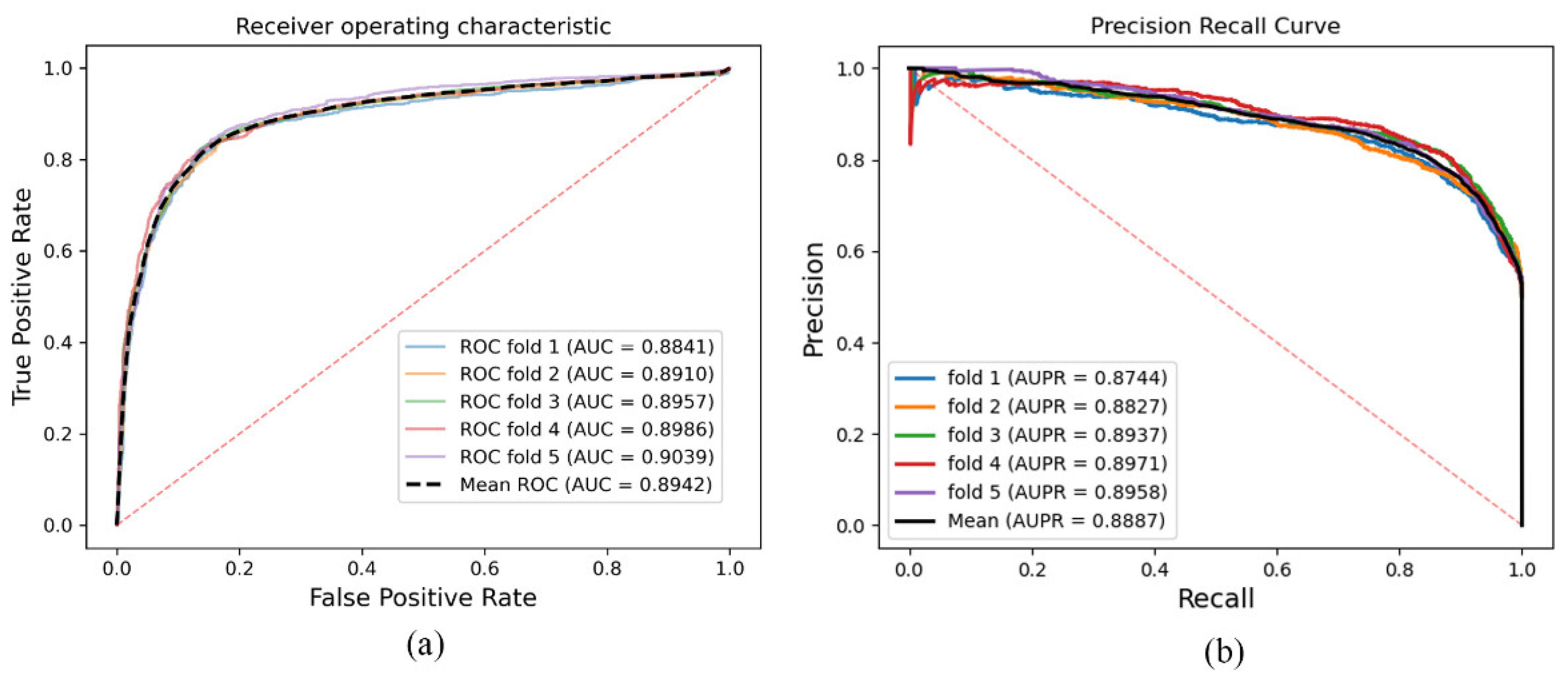
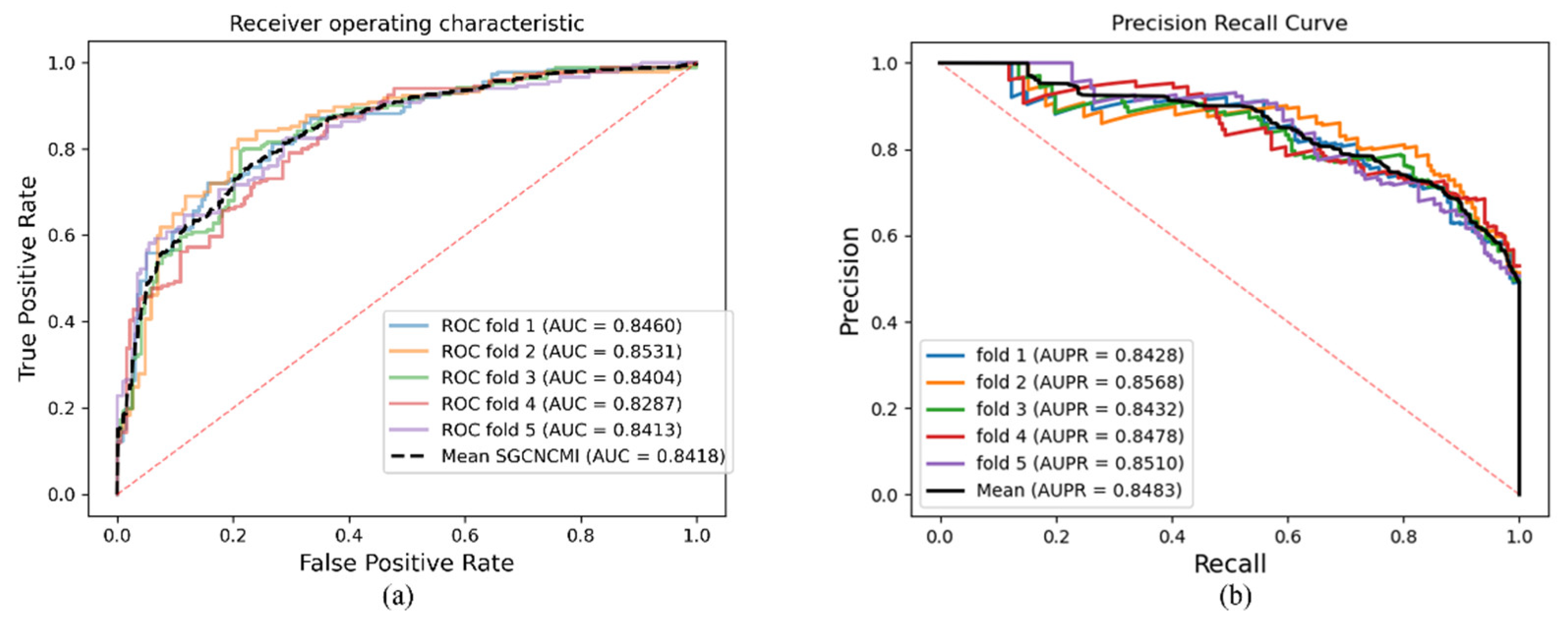
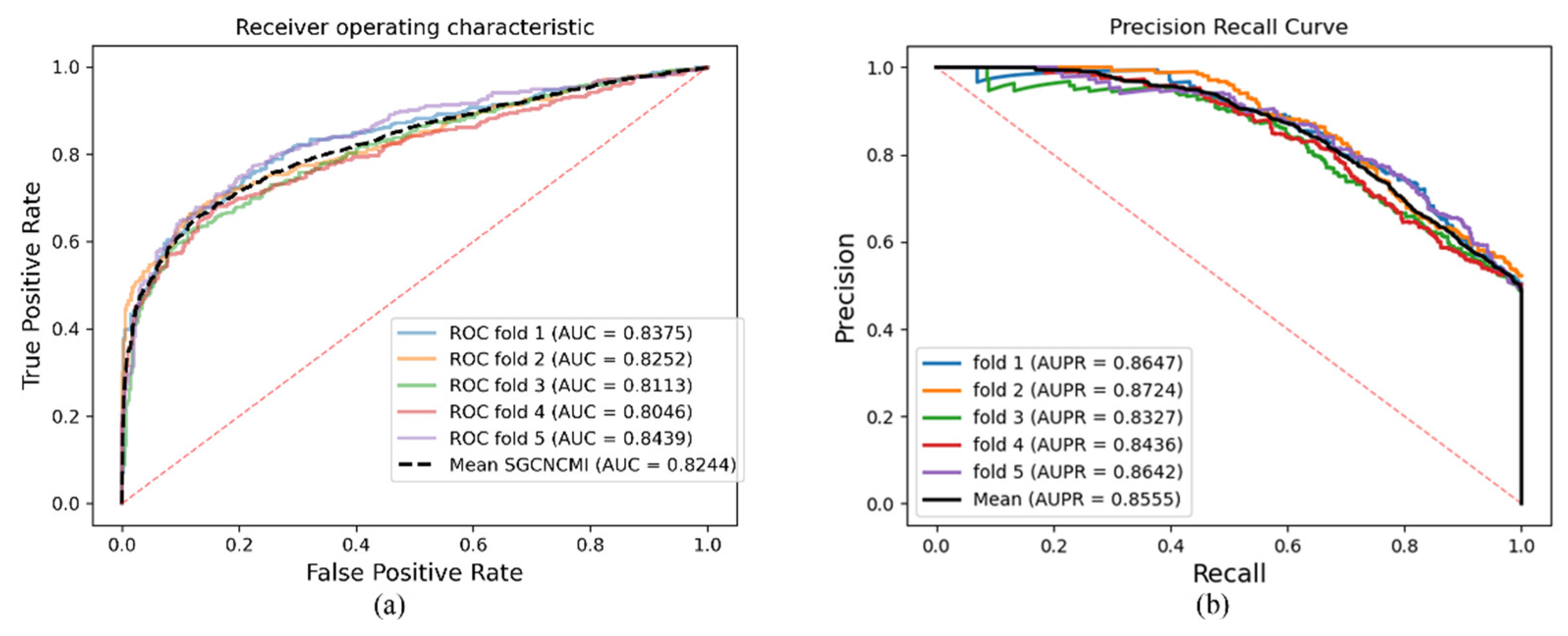
As a result, in a five-fold cross-validation experiment to measure the ability of the model, 89.42% AUC and 88.87% AUPR were obtained by SGCNCMI, and in the circRNA–miRNA interaction dataset test, the performance of SGCNCMI exceeded that of the only other model at present. In addition, 84.18% AUC and 84.83% AUPR were obtained by SGCNCMI in the circRNA–cancer dataset test, and 82.44% AUC and 85.55% AUPR were obtained in the circRNA–gene dataset. Meanwhile, 7 of the 10 pairs with the top predicted scores of the circRNA–miRNA interaction dataset test was verified in PubMed. Obviously, our model, SGCNCMI, is one of the few accurate and reliable prediction models in the field of circRNA–miRNA interaction prediction and is expected to become a powerful candidate model for biological experiments.
2. Materials and Methods
2.1. Dataset
As research progresses, a number of positive circRNA–miRNA correlations have been identified, and various databases have been established. The CircR2Cancer database [
24] is an online database that gathers experimentally validated circRNA–cancer and circRNA–miRNA associations reported in published papers. After rigorous screening, we obtained 318 circRNA–miRNA relational pairs between 238 circRNAs and 230 miRNAs.
At present, the techniques for predicting target gene binding sites are well developed, allowing the selection of candidates that closely match the binding sites, with high accuracy for most binding sites, and the vast majority of these predictions were eventually validated in subsequent experiments. Predicting target gene binding sites is already widely used in a variety of methods and tools; for example, CircInteractome [
25] uses a well-established TargetScan Perl script to analyze miRNAs that may be associated with circRNA. These data are extremely valuable. The circBank database [
22] performs binding site predictions for 140,790 human circRNAs and 1917 miRNAs using Miranda [
26] and TargetScan [
27] techniques, resulting in 42,917 relationships with more than five binding sites and 3545 relationships with more than one binding site. We selected the top 9589 pairs of circRNA–miRNA relationship pairs with the highest scores. These data were used in the first computational method [
28] in the field and partially validated in PubMed.
After combining data from both databases, we eventually obtained 9905 pairs of high-quality relationships for training in our methods, and for ease of description, we identified this dataset as CMI-9905.
To test SGCNCMI’s ability to predict the association between markers and underlying diseases, we downloaded 1049 experimentally supported circRNA–cancer relationship pairs from the Lnc2Cancer database [
29] of 743 circRNAs and 70 cancers.
In addition, we downloaded circRNA–gene-associated data from the TransCirc [
30] database and selected the top 2000 pairs with the highest confidence scores as training data.
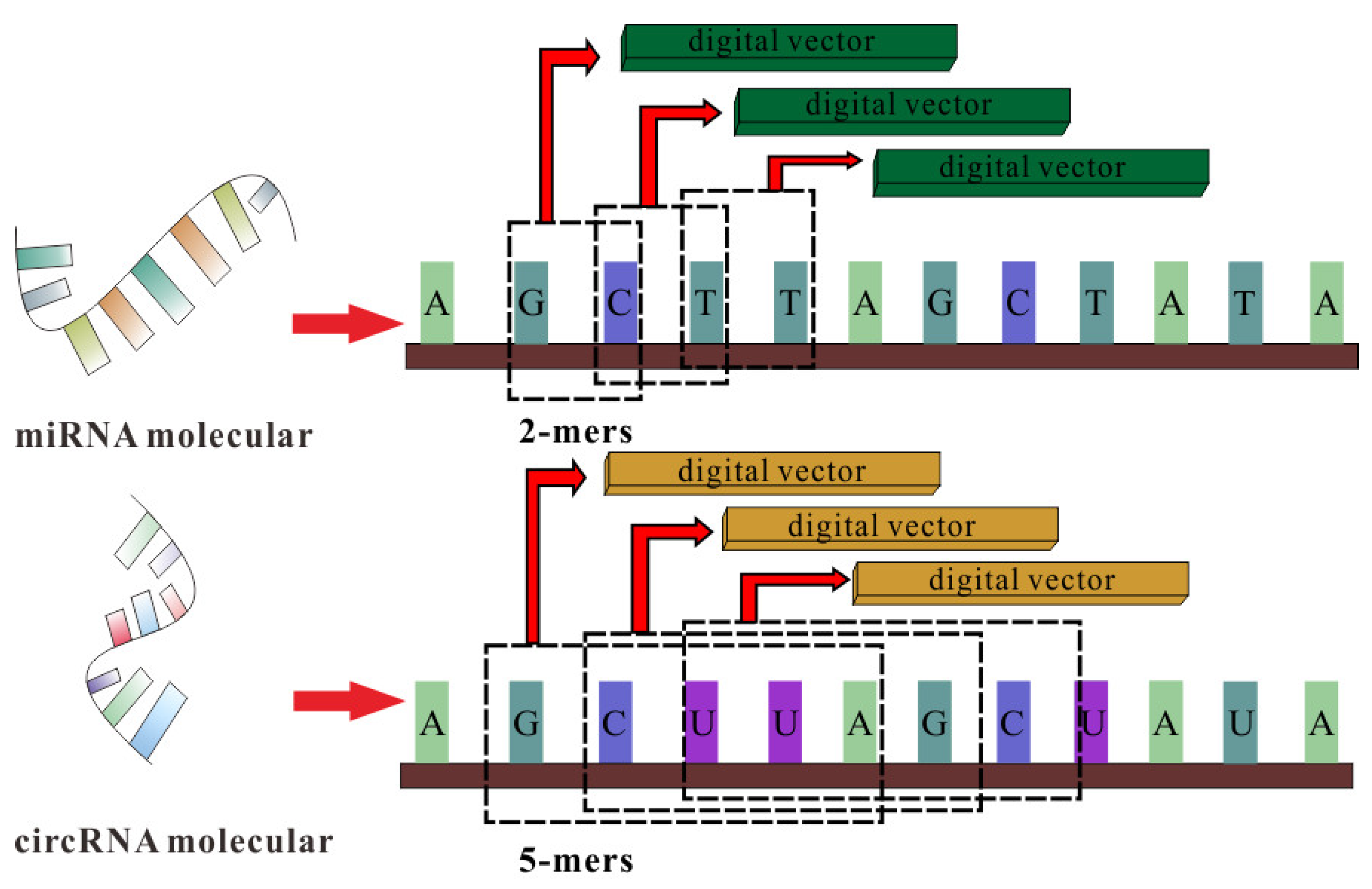
2.2. CircRNA and miRNA Sequence Similarity Based on K-mer
Counting RNA sequences’
K-mers (substrings of length k) is not only an important and common step in bioinformatics analysis but also widely used in computational methods [
31,
32]. Related studies have indicated that RNA sequences contain abundant biological information. Converting sequence information into a digital vector is an important method to obtain molecular biological information in order to fully explore hidden features in RNA sequences. The
K-mer sparse matrix is used to represent RNAs’ attribute features in our model.
For a circRNA sequence, we apply the best 5
-mers as the window to scan the sequence, moving one nucleotide at a time. Due to there being four different nucleotides in circRNA, the window of 5
-mers will produce 4
5 vector representations for each circRNA molecule. Therefore, the
K-mer matrix of circRNA can be represented as follows:
For a miRNA sequence, with an average length of 21 nucleotides, the scan window we use is 2
-mers to obtain the best vector representations, and the
K-mer matrix of miRNA is defined as:
The details of the
K-mer algorithm are shown in
Figure 1.
2.3. Similarity for CircRNA and miRNA
RNAs that can bind to the same molecule often have the same binding sites, which means that a potential unknown association can be inferred by analyzing RNA molecules with the same function. In order to fully express the biological characteristics of RNA molecules, we introduce two kinds of similarities (RNA Gaussian interaction profile kernel similarity and RNA sigmoid kernel similarity) as RNA semantic descriptors.
Firstly, we construct a bipartite graph
BC×M to represent the 9905 associations between circRNA and miRNA interaction pairs for 2346 circRNAs and 962 miRNAs. In the matrix
BC×M,
C and
M represent the number of circRNAs and miRNAs. When circRNA
i is related to miRNA
j, the value of
Bi×j is equal to 1 and otherwise equal to 0. Each row and column represent circRNA and miRNA interaction profiles, respectively; the interaction profile binary vector
LP(
Ci) of circRNA
Ci is the row corresponding to the circRNA in the adjacent matrix
BC×M, and the GIP kernel of each circRNA can be calculated as:
where
Ci and
Cj denote circRNA
i and circRNA
j, G
circRNA (
Ci,
Cj) is the GIP kernel similarity between circRNA
i and circRNA
j, and
αc is a variable parameter that controls the bandwidth of the GIP kernel, which is defined as follows:
In this experiment, αc’ is defined as equal to 0.5.
Similarly, the GIP kernel similarity between miRNA
mi and miRNA
mj is calculated as
The sigmoid kernel of each circRNA is defined as follows:
where
β = 1/V, and
V is the dimension of original input data.
In the same way, the sigmoid kernel of each miRNA is defined by the formula below:
2.4. Integrating Attributes and Similarity for circRNA and miRNA
Feature fusion can incorporate more meaningful information from different aspects, which can comprehensively reflect the characteristics of the circRNA and miRNA. In this section, we construct the characteristic fusion matrices of circRNA and miRNA. First, the different types of circRNA similarity (GIPKS and sigmoid kernel) matrixes are combined into one matrix called
FC(ci,cj) by the following formula:
In the same way, the miRNA similarity matrix is defined as
We integrate the attribute feature matrix and similarity feature matrix to obtain the heterogeneous network
HC×M as follows:
2.5. Node Feature Extraction Based on Sparse Autoencoder (SAE)
The features extracted from sequence and similarity often have information redundancy or “noise”. In this section, the Sparse Autoencoder (SAE) [
33] is used to reconstruct the eigenmatrix. As an unsupervised autoencoder, SAE can effectively learn the hidden features of input vectors, while the introduction of a sparsity penalty term can also learn relatively sparse features well.
SAE is an unsupervised encoder including an input layer hidden layer and output layer. The input layer maps the input data
X to the hidden layer
Lh for encoding, where layer
Lh is defined as follows:
where
X(i) is the original input data, WL is a connection parameter between the input and hidden layers, and
bLi represents an offset of function.
SAE defines
σ() as the activate function, which can be represented as:
The average activation of the activated hidden units can be calculated as:
where
αh() denotes the activation amount of the hidden units.
The sparsity penalty term
Ps is added to the target function to keep the hidden layer at low average activation values, which are shown as:
where
Ps is the sum of the degrees of penalization,
deviates from
ρ, and
Ln represents the number of units in the hidden layer. KL divergence (Kullback–Leibler) represents the sparsity penalty term of SAE and is defined as follows:
where
ρ is the sparsity parameter of
KL, which is close to 0; when
is closer to
ρ, the value of
KL is smaller, and when
is equal to
ρ, KL is equal to 0; otherwise, it increases monotonically.
With the sparsity penalty term added, the cost function is defined as:
where
δ is the weight of the sparsity penalty term, and
CL(w, b) is the cost function of each layer, which is calculated by the backpropagation algorithm:
where
ϑ denotes the learning rate of the neural networks.
In this work, the heterogeneous network H is processed by SAE as the input data, and the final characteristic matrix DC×M is generated, where each row of DC×M represents the attribute characteristics of the corresponding node.
2.6. SGCNCMI
According to the effective application of graph neural networks in the prediction field, we propose a novel prediction model (SGCNCMI) based on a graph convolutional neural network. SGCNCMI can be described in the following six steps: (1) construct a circRNA–miRNA adjacency matrix, (2) use the RNA sequence and functional similarity to generate the node attribute feature representation, (3) use the Sparse Autoencoder (SAE) to further extract features and generate the final node feature representation, (4) apply GCN to map the relationship network diagram to a new space so as to aggregate the features of potentially associated nodes, (5) apply the weighted cross-entropy loss function to train the whole model in an end-to-end manner, and (6) apply an inner product decoder to score each pair of relationships. Next, the implementation details for each step are shown.
In step 1, we integrated known circRNA–miRNA interactions into an adjacency matrix, which contained 9905 processed high-quality interaction pairs between 2346 circRNAs and 962 miRNAs. We treated all of these 9905 interaction pairs as positive edges between circRNA nodes and miRNA nodes, and we also randomly constructed 9905 negative samples to balance the training set to better train the model. Then, all of the positive edges were labeled 1, and all of the negative samples were labeled 0.
In step 2, in order to fully express the attributes of nodes, we tried to combine multi-source information to extract node features and convert the features into digital vectors. First, related studies have confirmed that RNA molecular sequences contain abundant biological attribute information, and we applied the K-mer algorithm to process sequences to obtain the underlying feature representation. Due to the difference in the length of RNA sequences, we used 5-mers for circRNA and 2-mers for miRNA, and finally, we obtained a 128-dimension circRNA sequence vector and a 16-dimension miRNA sequence vector. Next, based on the assumption that circRNAs with similar functions are likely to be related to miRNAs with similar phenotypes, we increased two kinds of similarity (RNA Gaussian interaction profile kernel similarity and RNA sigmoid kernel similarity) to construct the comprehensive similarity matrix.
In step 3, we used SAE to further process the preliminary multidimensional features. SAE is an unsupervised autoencoder with sparsity penalty terms that can effectively extract potential features from a matrix with redundant information, while the introduction of the sparsity penalty term can obtain more valuable information from the sparse matrix. Finally, we obtained the comprehensive characteristics vectors of each node as below:
where
ci represents the features of circRNA
i, and
mj represents the features of miRNA
j.
In step 4, we transformed the prediction of circRNA–miRNA association into a link prediction problem on a heterogeneous bipartite graph, and GCN was used to effectively learn latent graph structure information and the representations of node attributes from an end-to-end model structure. First, for an undirected heterogeneous bipartite graph
A, self-connections were added to ensure nodes’ characteristic contributions:
where
A is the bipartite graph, and I is the identity matrix. In order to promote the contribution of the association relation in the propagation process of the graph convolutional network, we normalized matrix
as follows:
where
is calculated as:
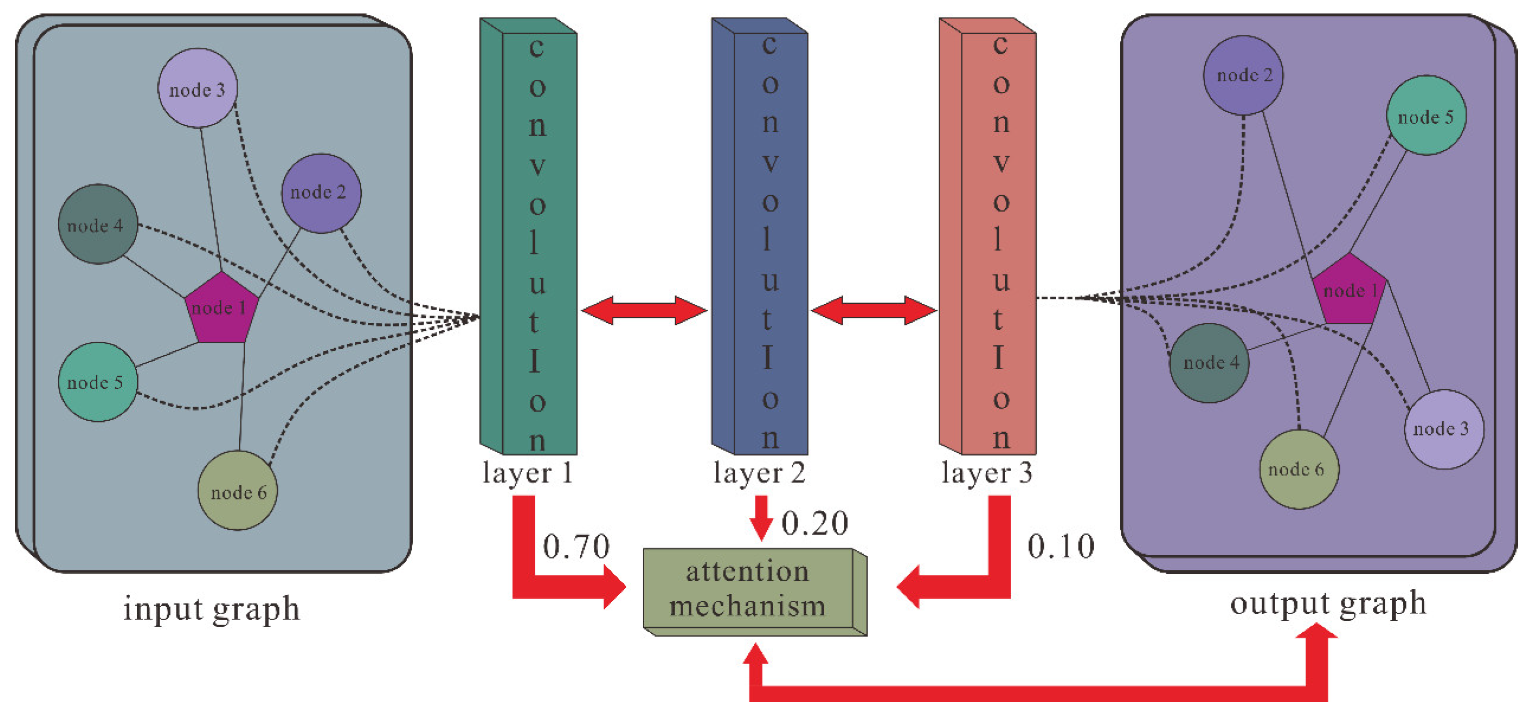
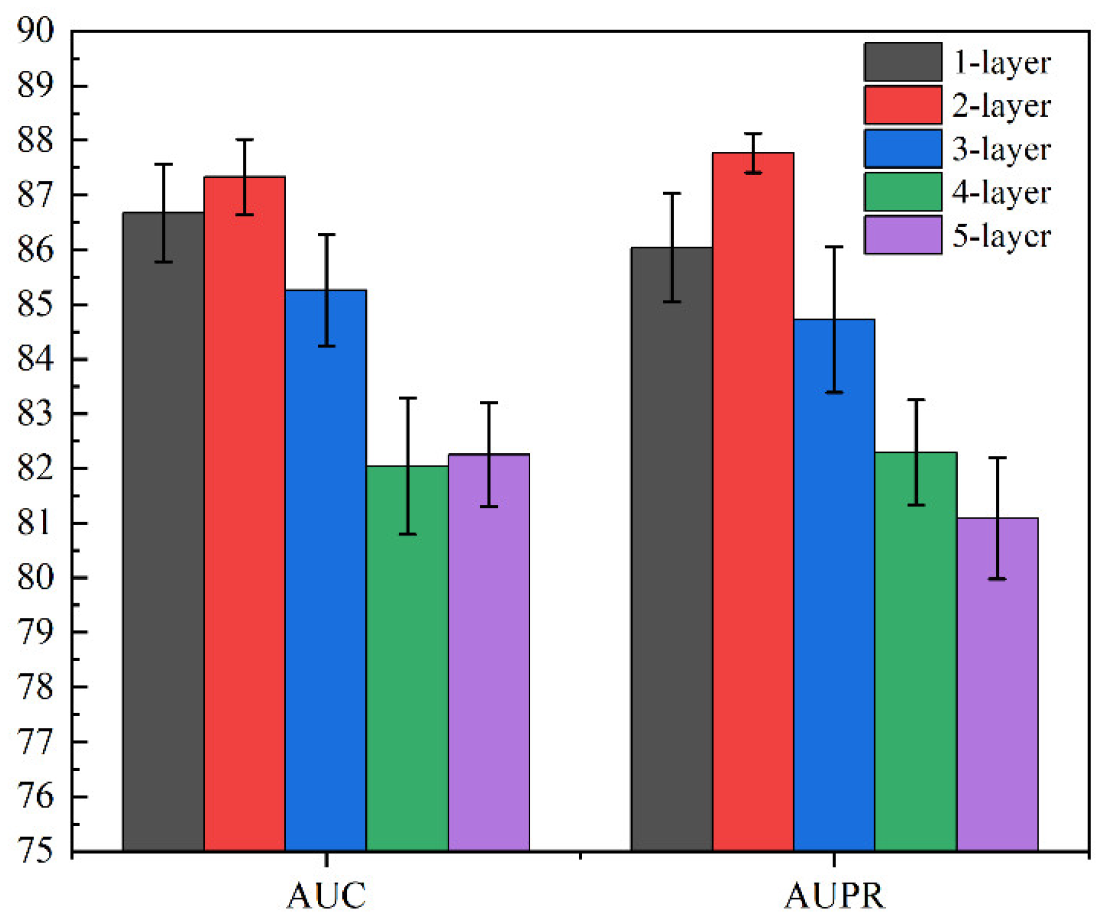
Then, we utilized GCN containing three layers of graph convolutional networks to aggregate node features and generate a corresponding lower-dimensional feature matrix. The specific process is shown in the following formulas:
where
H(l) represents the node feature vector of the lth layer, and
H(0) is the comprehensive characteristics vector of each node that is extracted by SAE.
W(l) is the lth layer trainable weight matrix, and
σ() denotes the ReLU activation function. Meanwhile, to solve the problem that the contributions of different layers’ embeddings are unequal, we introduce the attention mechanism, which is defined as follows:
where
nl is the weight parameter, which is auto-learned by the graph convolutional network, and
Mcm is the final embedding representation obtained by GCN. The GCN extraction process is shown in
Figure 2.
In step 5, we applied weighted cross-entropy as a loss function to train the model. The loss function is defined as follows:
where ω represents a weight parameter, which is equal to the ratio of negative samples to positive samples. This function is used to calculate the weighted cross-entropy between the true value of the label b and the target b* obtained by the model’s internal product algorithm.
Figure 2 shows the GCN processing flow.
In step 6, the inner product algorithm based on the principle of matrix factorization (MF) was used to obtain the final score of each pair, and the reconstructed score matrix can be calculated as follows:
The detailed process of SGCNCMI is shown in
Figure 3.
In addition, our model directly uses the similarity of a marker to disease as an attribute feature when predicting the relationship between markers and underlying diseases due to the absence of molecular sequences. This makes our model more functional and robust as a predictor of both states.

 and
and 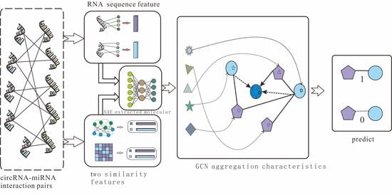


