
Study of 3-D Prandtl Nanofluid Flow over a Convectively Heated Sheet: A Stochastic Intelligent Technique

 , ,
, ,  ,
,  and
and
Abstract
:1. Introduction
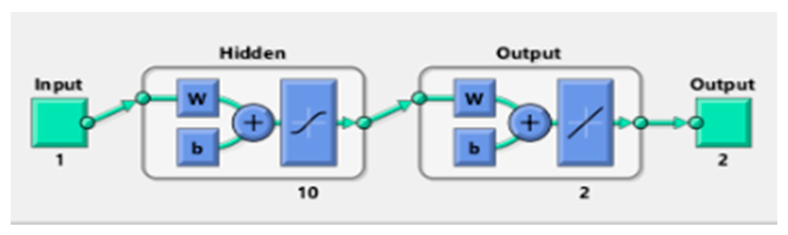
- The numerical computation has been designed through the technique of Levenberg Marquardt with backpropagated artificial neural network (TLM-BANN) for the comparative study of three dimensional Prandtl nanofluid flow model (TD-PNFM) with convectively heated surface.
- The TLM-BANN coupled PDEs representing TD-PNFM are transformed into system of ODEs by utilizing suitable transformation.
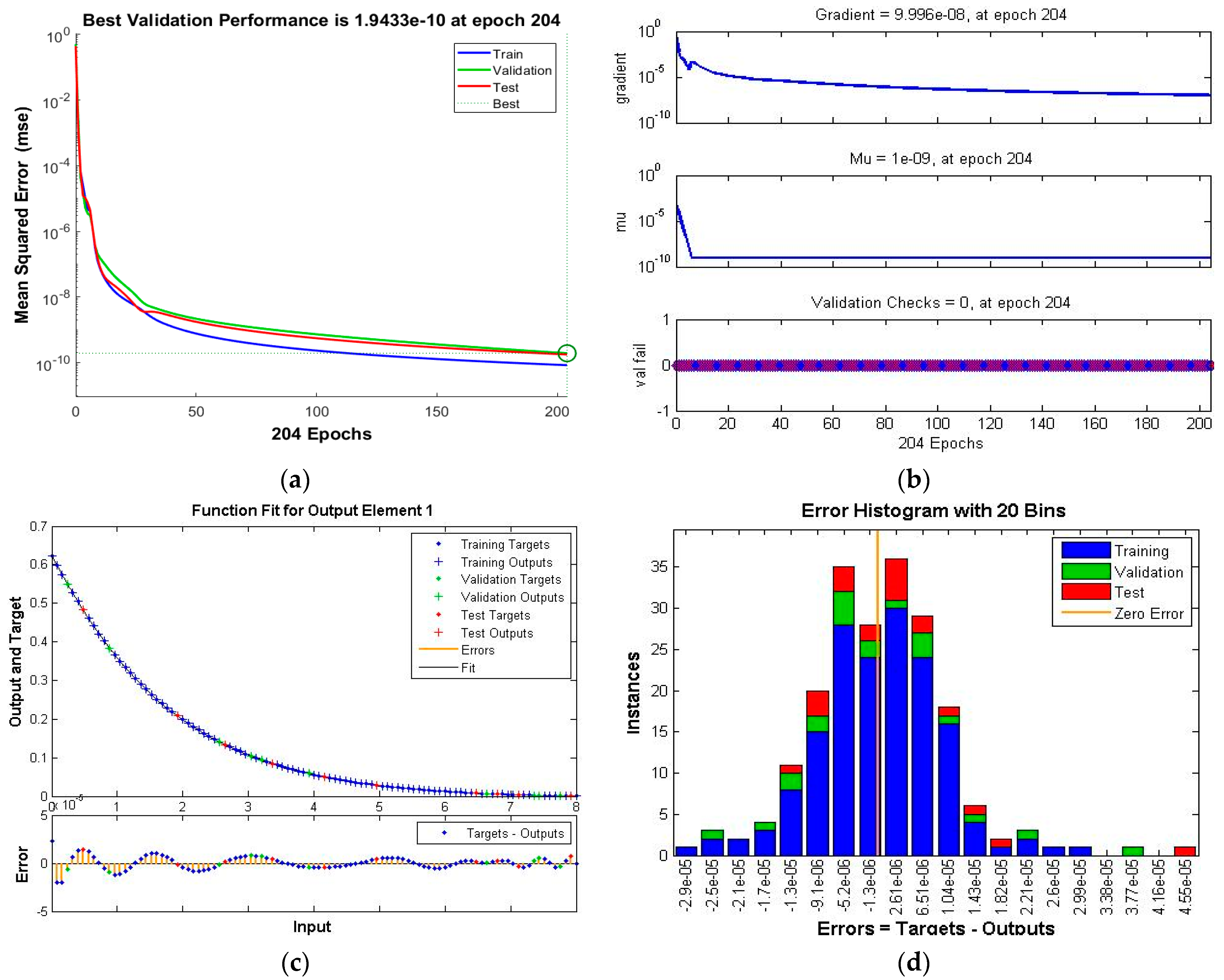
- The Mathematica software command ‘NDSolve’ is used to compute the dataset for designed TLM-BANN for the variation of Prandtl fluid number, flexible number, ratio parameter, Prandtl number, Biot number and thermophoresis number.
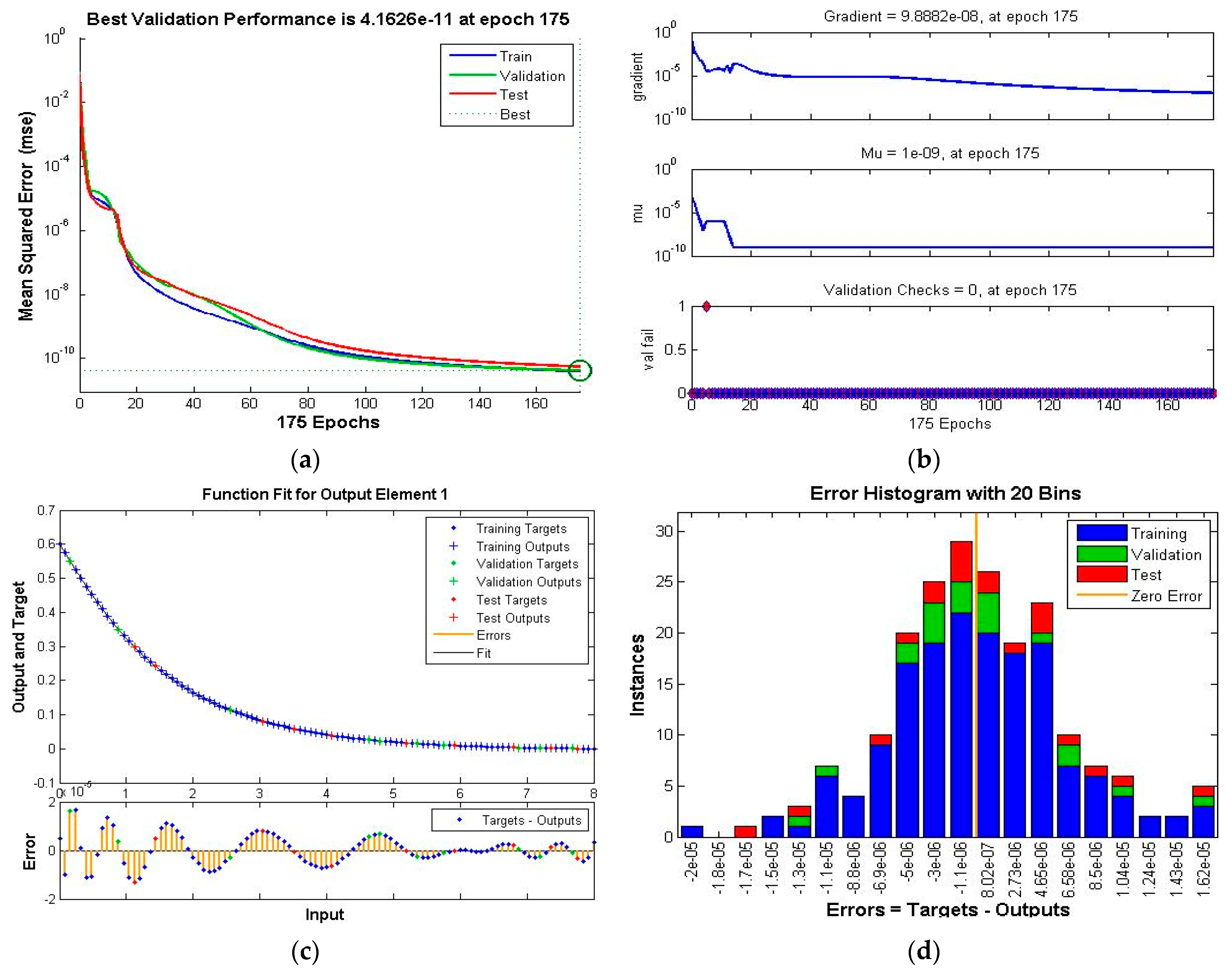
- The MATLAB software is used to interpret the solution and the AE analysis plots of TD-PNFM.
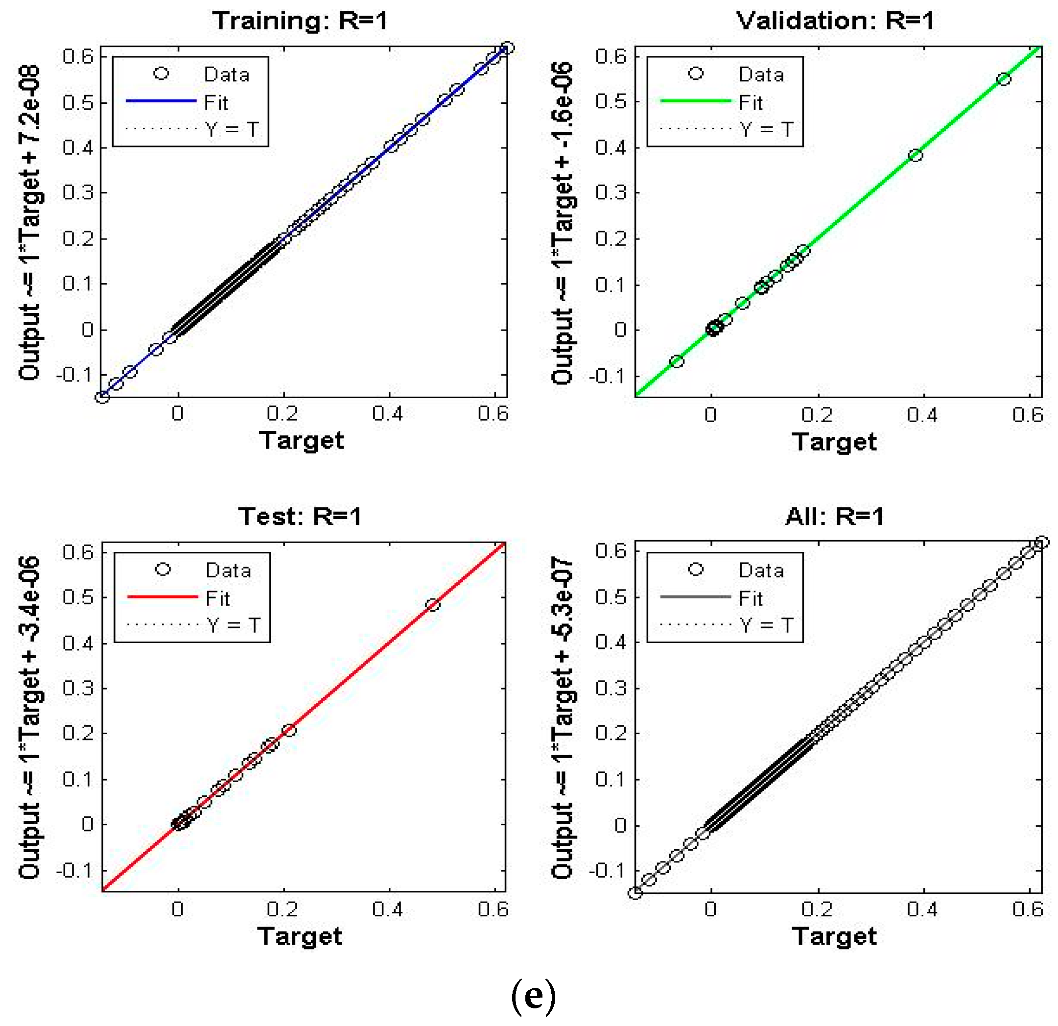
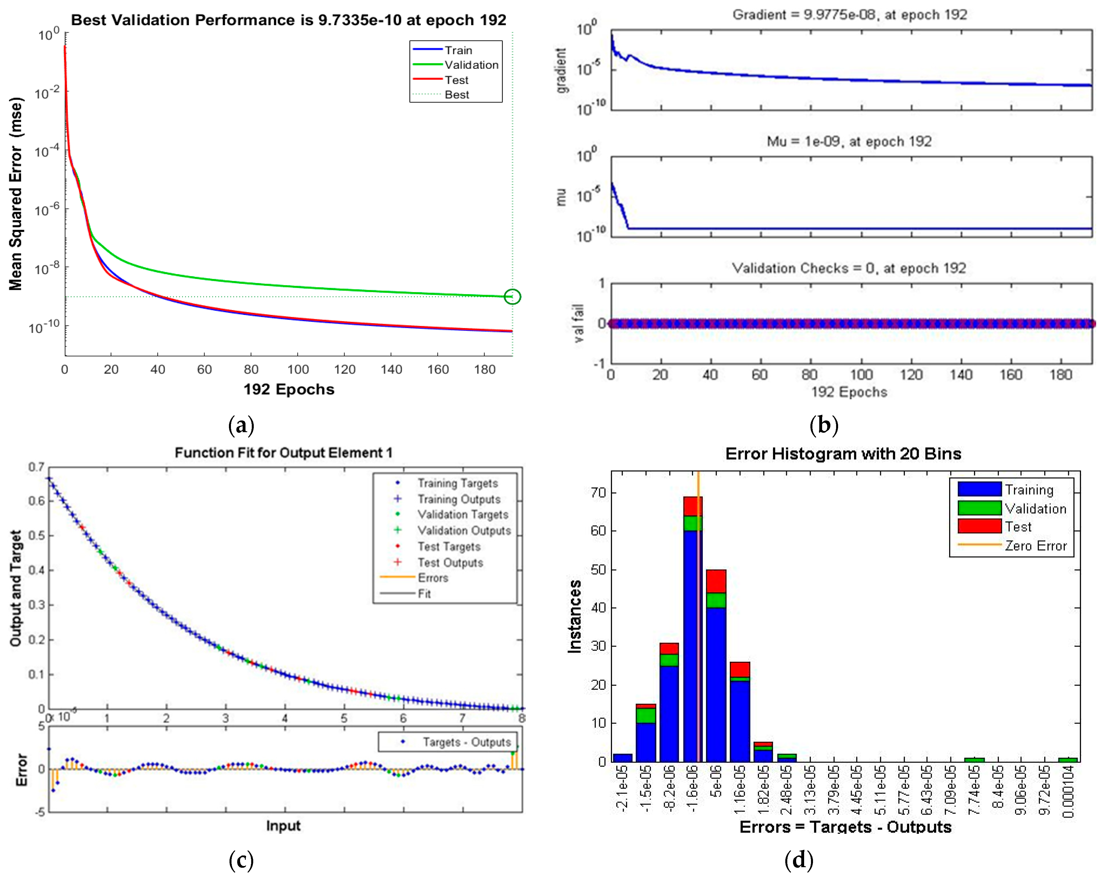
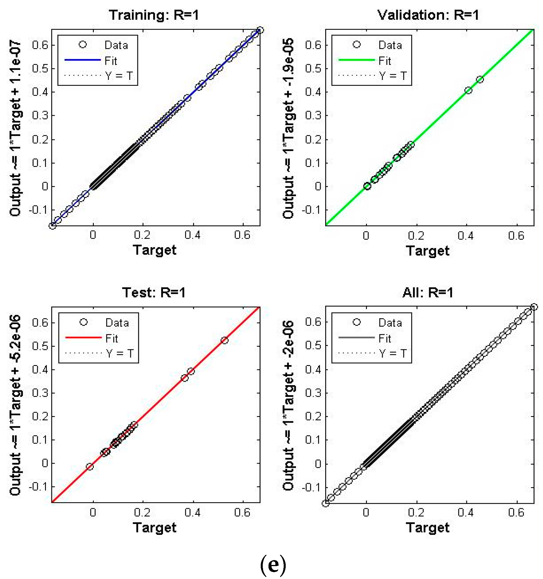
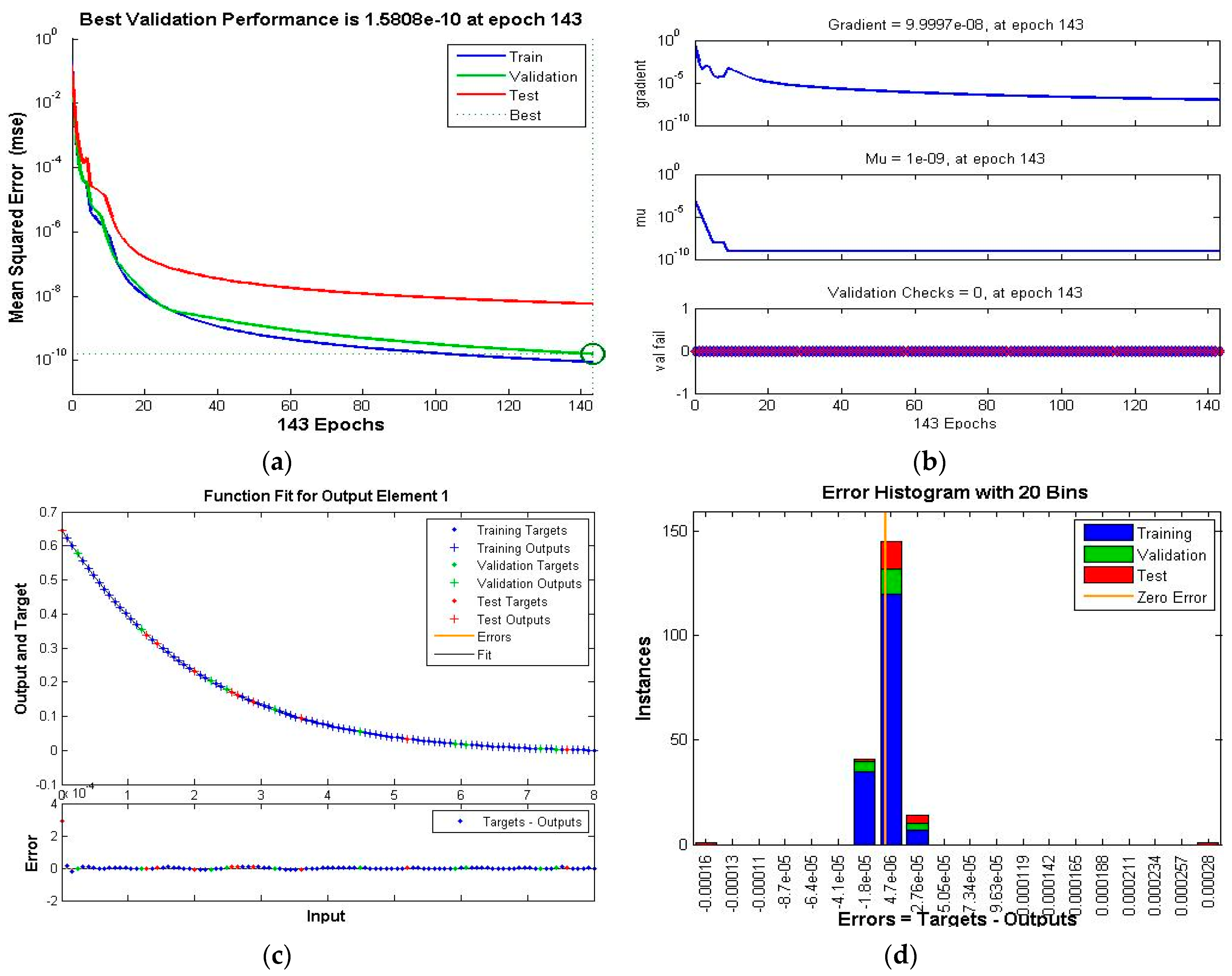
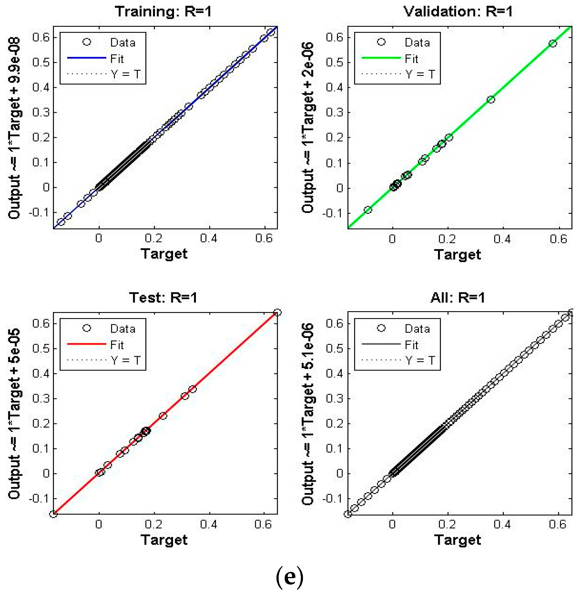
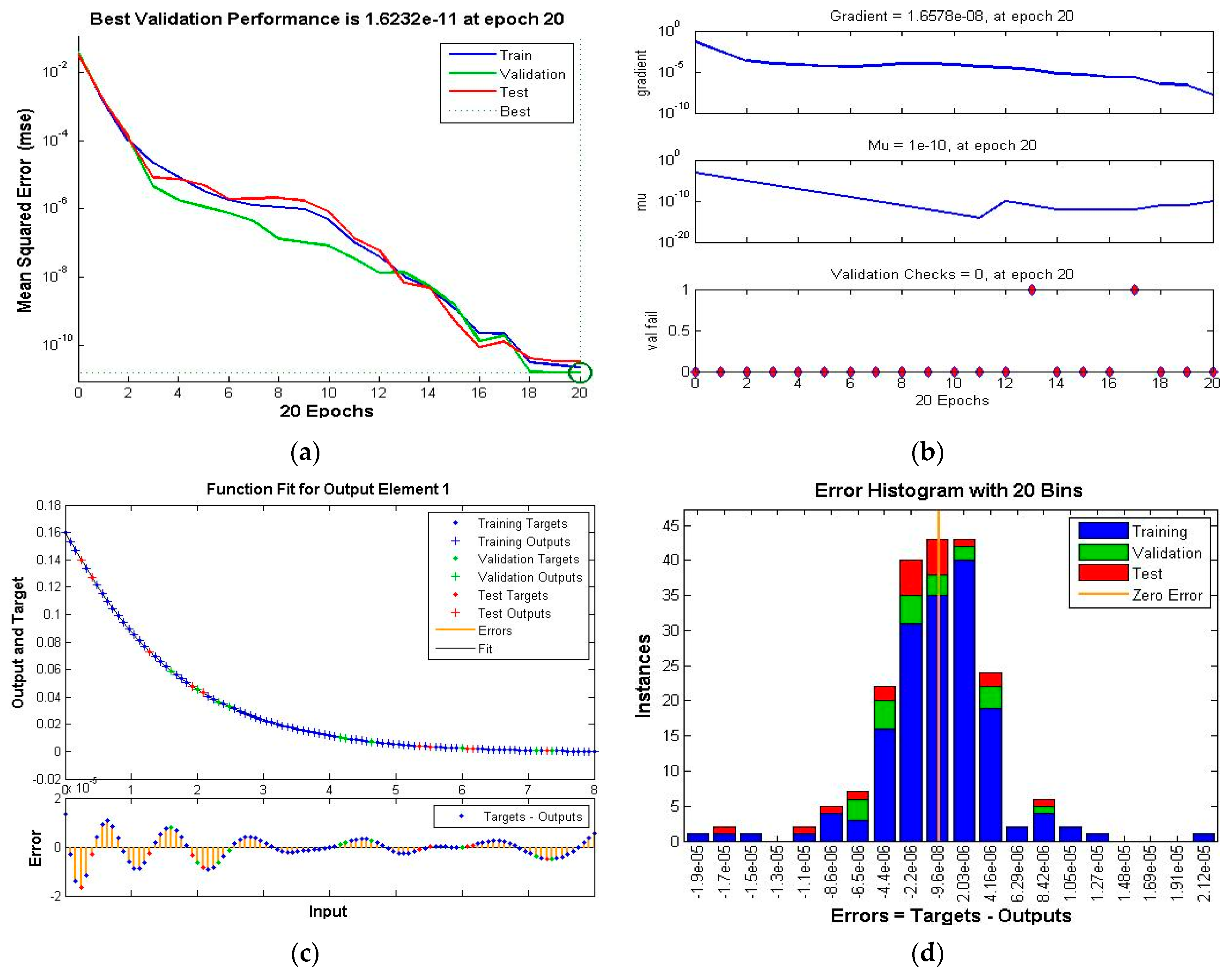
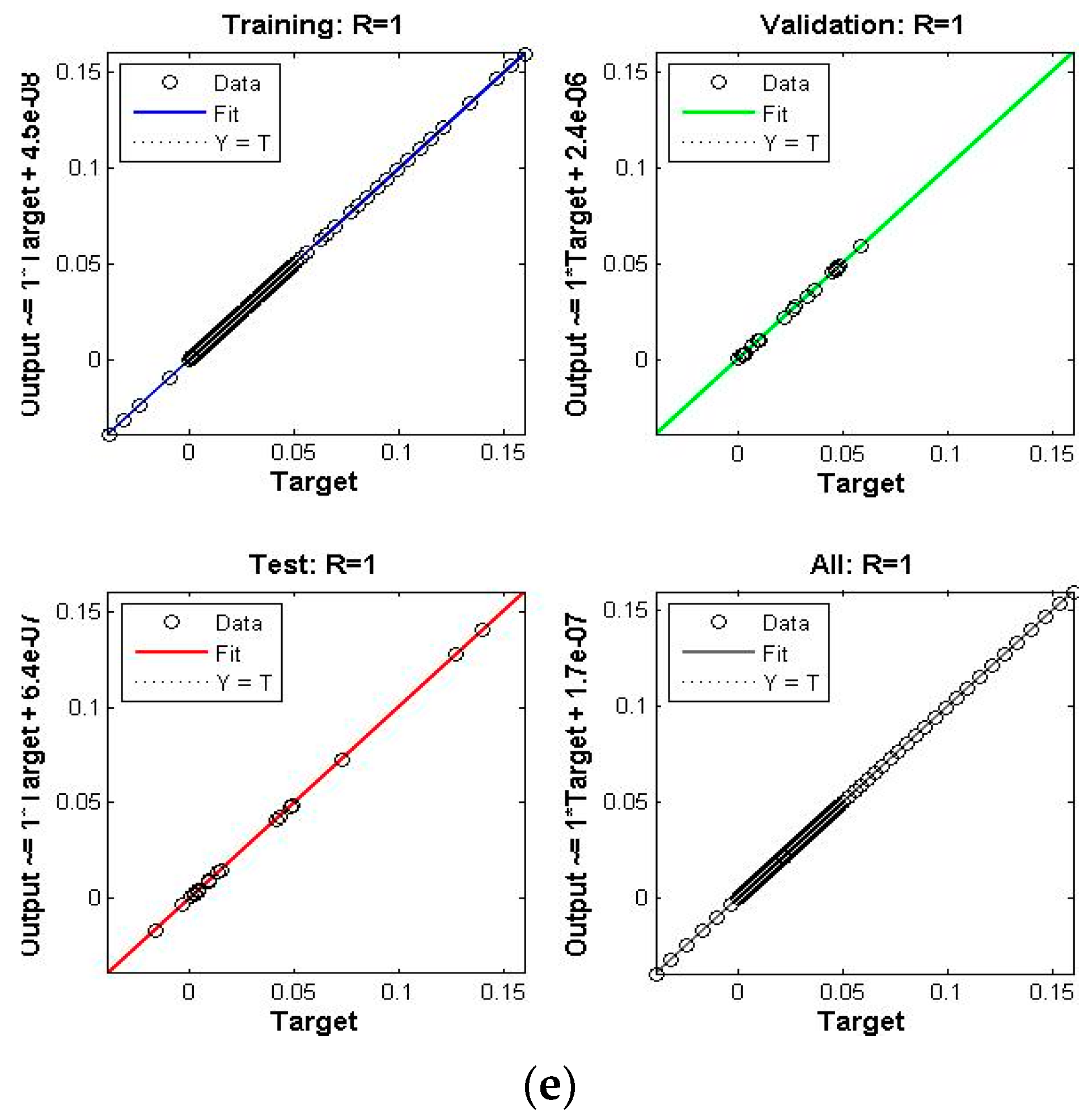
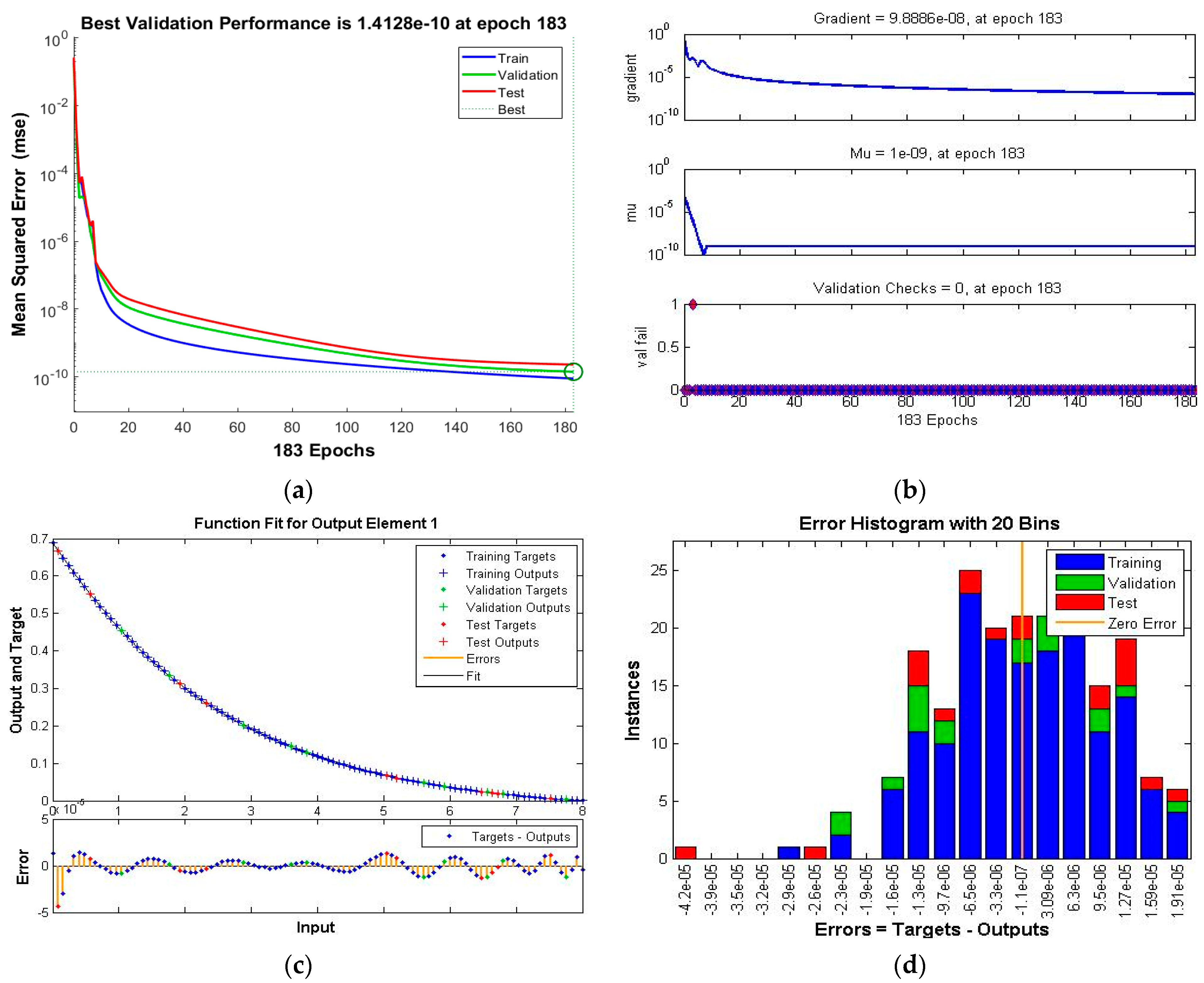
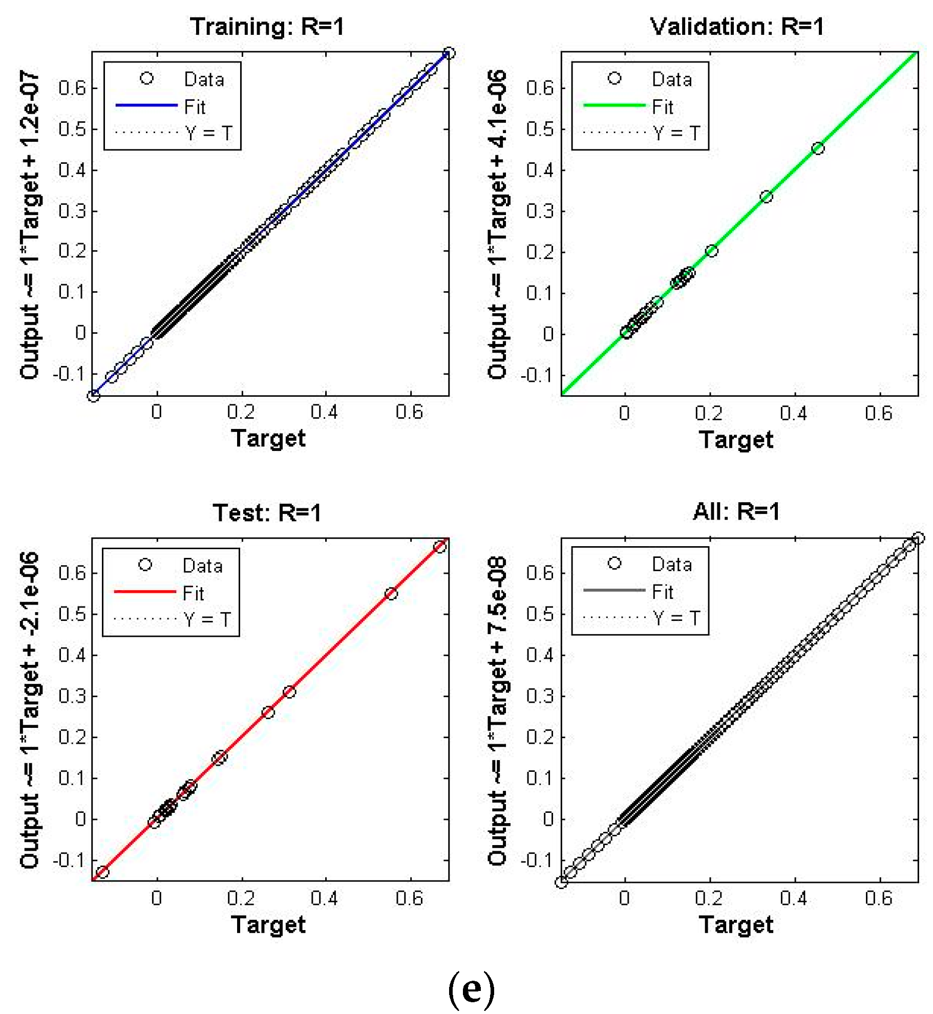
- The correctness and the validation of the proposed TD-PNFM is examined by training, testing and validation process of TLM-BANN.
- Regression analysis, error histogram and results of mean square error (MSE), validates the performance analysis of designed TLM-BANN.
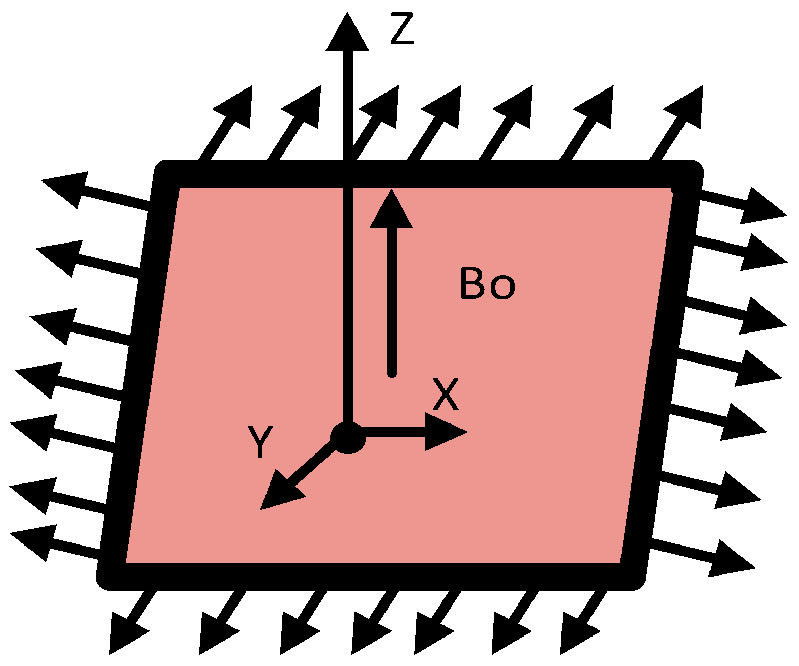
2. Mathematical Modeling
3. Solution Methodology
4. Discussion of Results
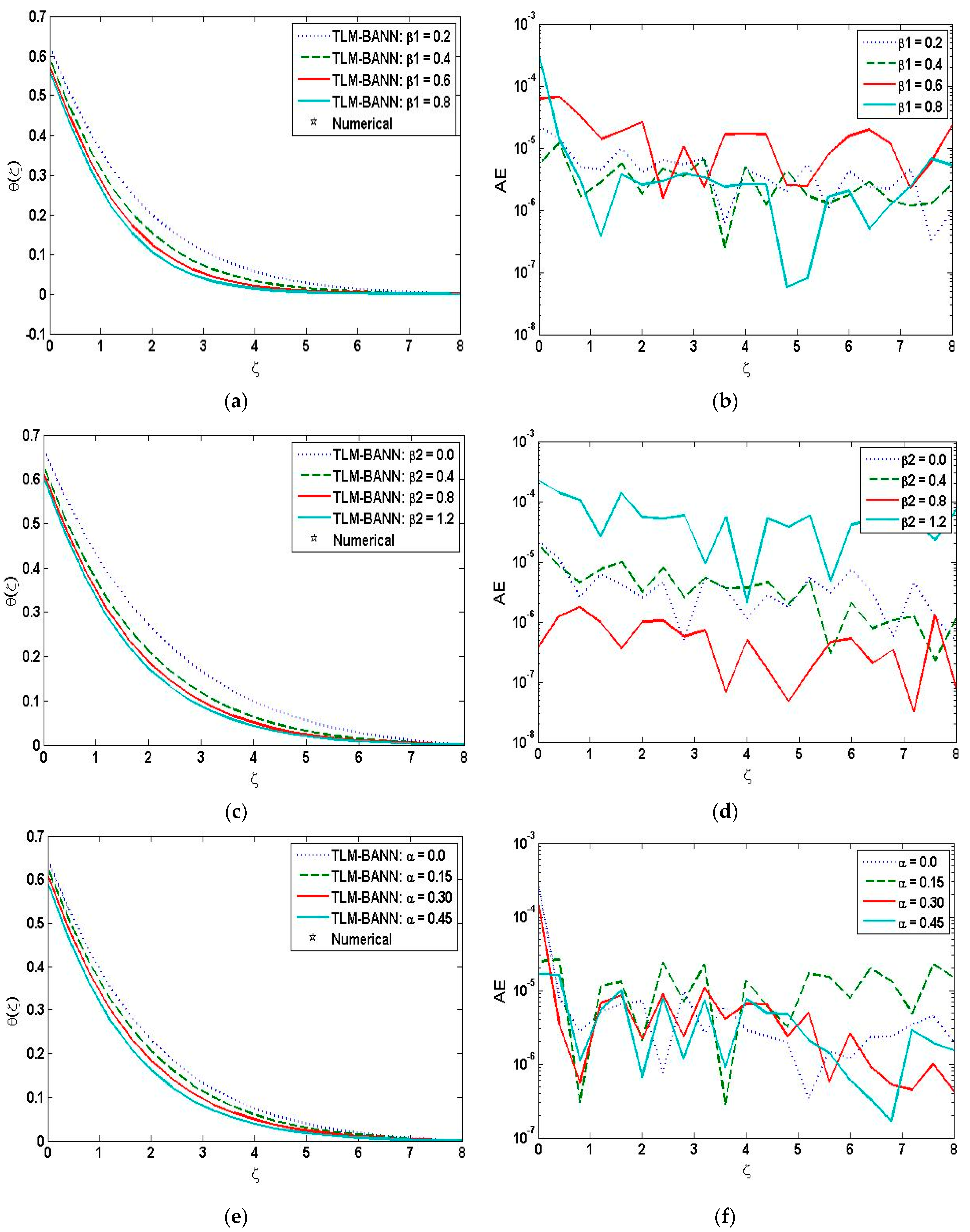
4.1. Impact of Variation on θ(ζ)
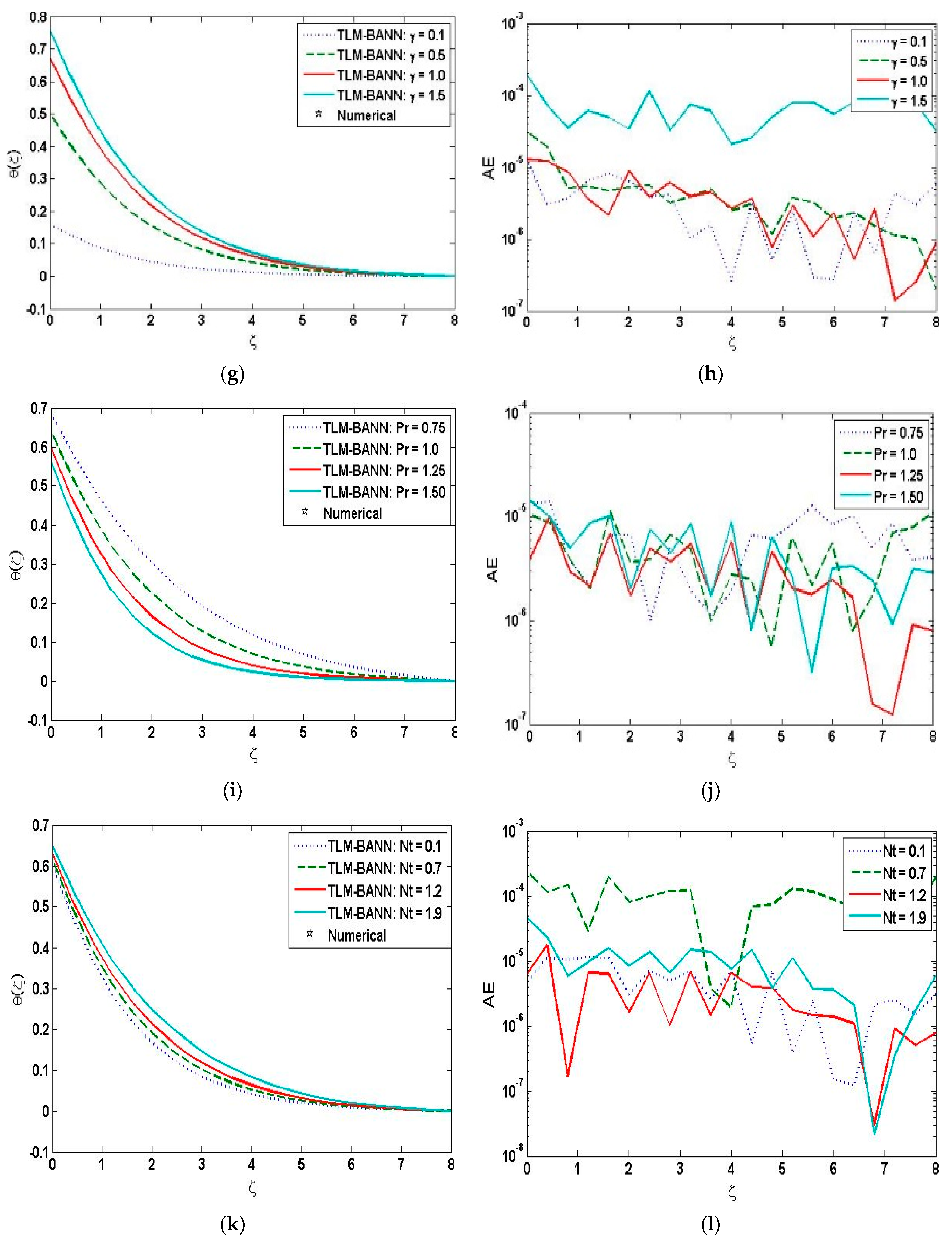
- The temperature profile increases with the increase in Biot number.
- Temperature distribution shows decreasing behavior with the increase in Prandtl fluid number and flexible number.
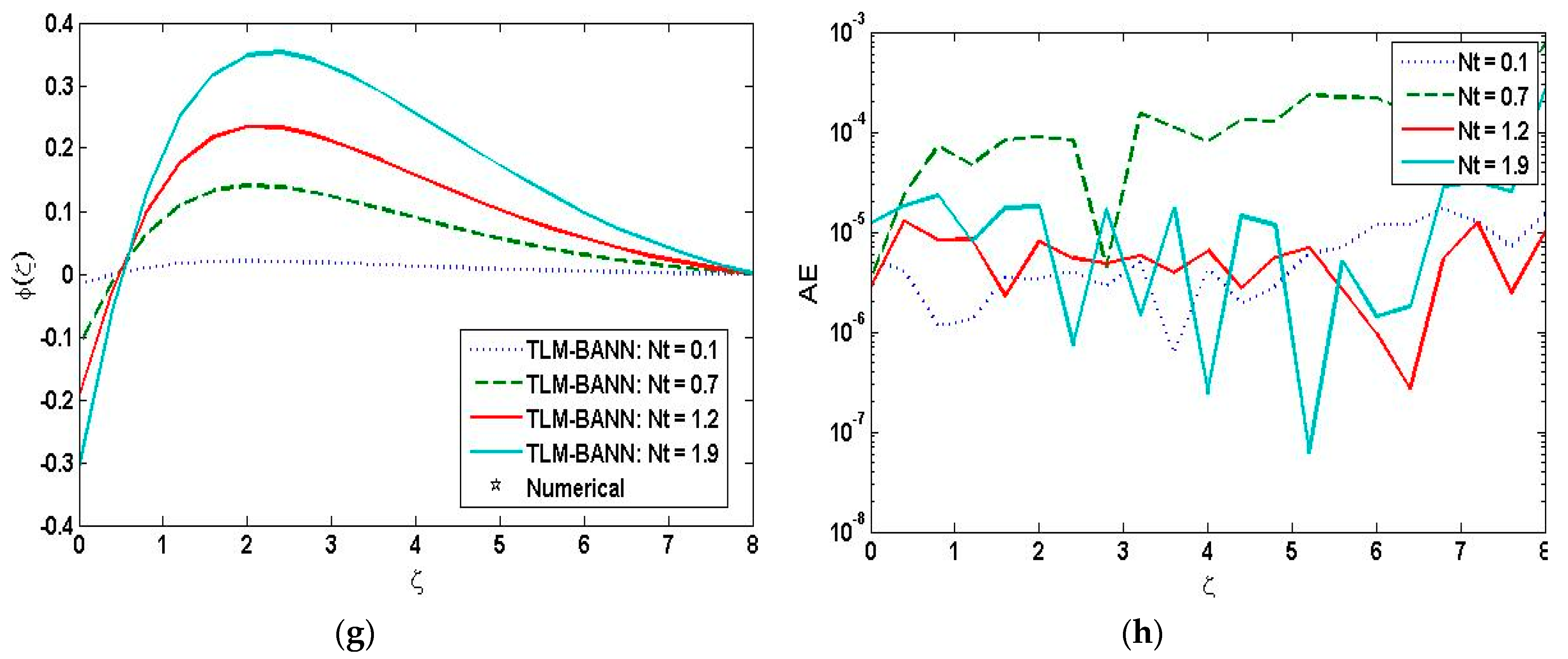
- Increase in thermophoresis number leads to an increase in temperature profile.
- Temperature profile decreases with the increase in the values of Prandtl number and ratio parameter.
4.2. Impact of Variation on
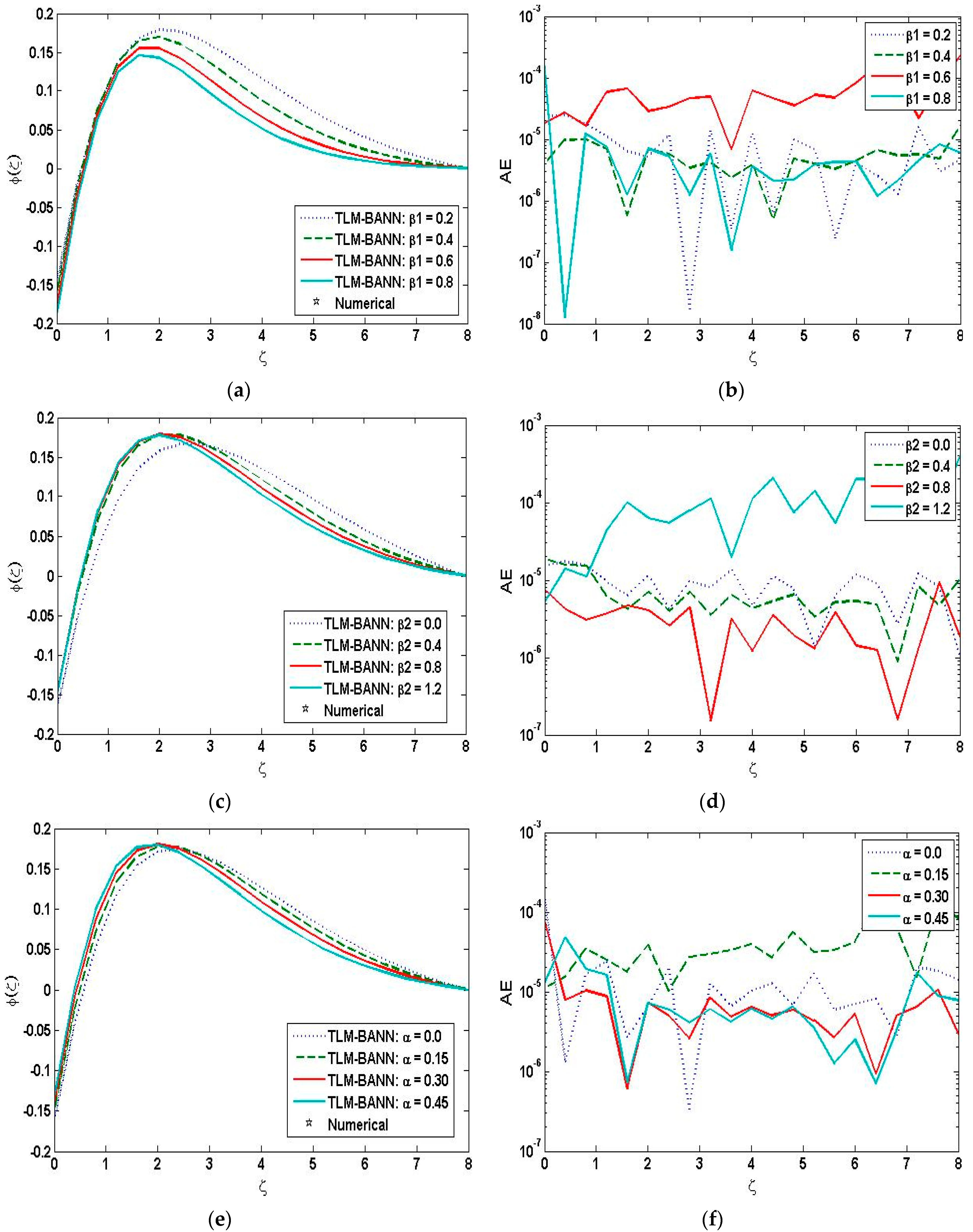
- The concentration profile shows decreasing behavior when the value of Prandtl fluid parameter increases.
- Increase in flexible number causes a decrease in concentration profile.
- Increasing values of ratio parameter leads to a decrease in the behavior of concentration profile.
- The concentration profile increases with the increase in thermophoresis parameter. The reason is, raising thermophoresis parameter induces a rise in the system’s thermal conductivity, which adds to an increase in concentration.
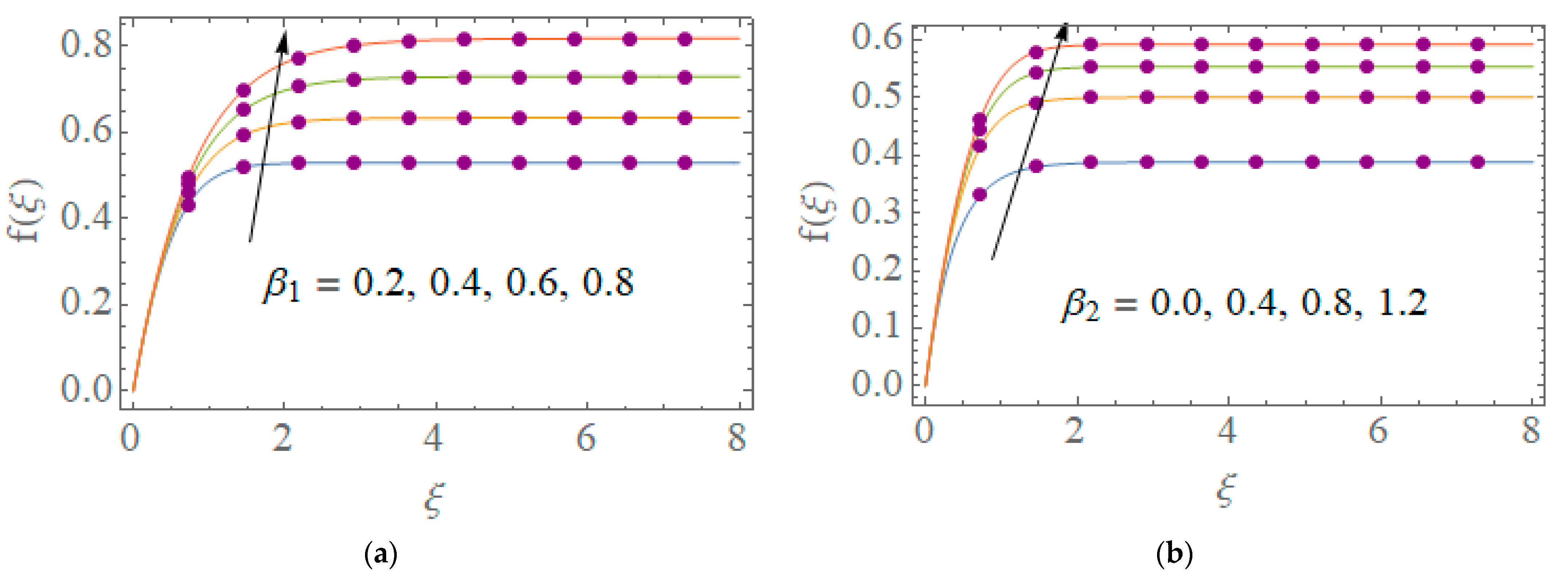
4.3. Impact of Variation on f(ζ)
- Velocity distribution shows an increasing trend with the increase in Prandtl fluid number.
- Increase in flexible number leads to an increase in velocity profile.
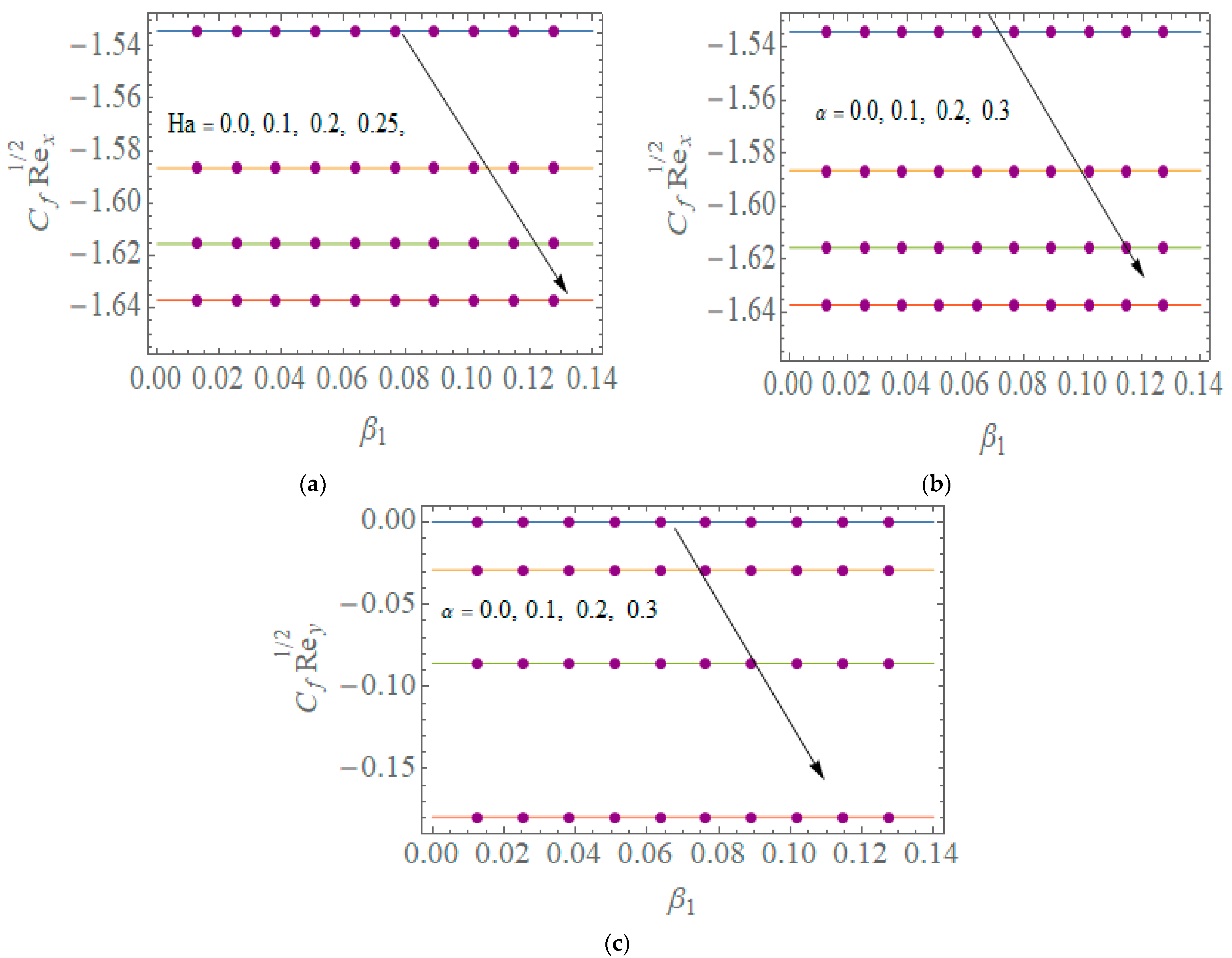
4.4. Skin Friction Coefficient
- shows a declining trend with the increase in Hartmann number and ratio parameter against Prandtl fluid parameter.
- Rise in ratio parameter leads to a decrease in against Prandtl fluid parameetr.
4.5. Nusselt Number
- shows a falling pattern with the increase in thermophoresis parameter against Brownian motion parameter.
5. Conclusions
- The temperature profile shows increasing behavior with the increase in Biot number.
- Temperature distribution is decreasing with the increase in Prandtl fluid number and flexible number.
- Increase in thermophoresis number leads to an increase in temperature profile.
- Temperature profile decreases when the values of Prandtl number and ratio parameter increase.
- The concentration profile decreasing when the value of Prandtl fluid parameter increases.
- Increase in flexible number causes a decrease in concentration profile.
- Increasing values of ratio parameter causes a decrease in concentration profile.
- The concentration profile increases with the increasing values of thermophoresis parameter.
- Velocity distribution shows an increasing trend for the upsurge in the values of Prandtl fluid parameter and flexible parameter.
- Skin friction coefficient declines for the increase in Hartmann number and ratio parameter
- Nusselt number falls for the rising values of thermophoresis parameter against Nb.
6. Future Work
Author Contributions
Funding
Institutional Review Board Statement
Informed Consent Statement
Data Availability Statement
Acknowledgments
Conflicts of Interest
Nomenclature
| β1 | Prandtl fluid number |
| α | Ratio parameter |
| Pr | Prandtl number |
| γ | Biot number |
| Nb | Brownian motion parameter |
| Nt | Thermophoresis Parameter |
| TD-PNFM | three dimensional Prandtl nanofluid flow model |
| Sc | Schmidt number |
| θ | Temperature profile |
| φ | Concentration profile |
| Ha | Hartman number |
| β2 | Flexible number |
| MSE | Mean square error |
| TLM-BANN | technique of Levenberg Marquardt with backpropagated artificial neural network |
References
- Choi, S.U.; Eastman, J.A. Enhancing Thermal Conductivity of Fluids with Nanoparticles (No. ANL/MSD/CP-84938; CONF-951135-29); Argonne National Lab: Argonne, IL, USA, 1995.
- Wang, X.Q.; Mujumdar, A.S. Heat transfer characteristics of nanofluids: A review. Int. J. Ther. Sci. 2007, 46, 1–19. [Google Scholar] [CrossRef]
- Das, S.K.; Choi, S.U.; Patel, H.E. Heat transfer in nanofluids—A review. Heat Transf. Eng. 2006, 27, 3–19. [Google Scholar] [CrossRef]
- Wen, D.; Lin, G.; Vafaei, S.; Zhang, K. Review of nanofluids for heat transfer applications. Particuology 2009, 7, 141–150. [Google Scholar] [CrossRef]
- Duangthongsuk, W.; Wongwises, S. Heat transfer enhancement and pressure drop characteristics of TiO2–water nanofluid in a double-tube counter flow heat exchanger. Int. J. Heat Mass Transf. 2009, 52, 2059–2067. [Google Scholar] [CrossRef]
- Leong, K.Y.; Saidur, R.; Kazi, S.N.; Mamun, A.H. Performance investigation of an automotive car radiator operated with nanofluid-based coolants (nanofluid as a coolant in a radiator). Appl. Ther. Eng. 2010, 30, 2685–2692. [Google Scholar] [CrossRef]
- Saidur, R.; Leong, K.Y.; Mohammed, H.A. A review on applications and challenges of nanofluids. Renew. Sust. Energ. Rev. 2011, 15, 1646–1668. [Google Scholar] [CrossRef]
- Yousefi, T.; Shojaeizadeh, E.; Veysi, F.; Zinadini, S. An experimental investigation on the effect of pH variation of MWCNT–H2O nanofluid on the efficiency of a flat-plate solar collector. Sol. Energ. 2012, 86, 771–779. [Google Scholar] [CrossRef]
- Kakaç, S.; Pramuanjaroenkij, A. Review of convective heat transfer enhancement with nanofluids. Int. J. Heat Mass Transf. 2009, 52, 3187–3196. [Google Scholar] [CrossRef]
- Turkyilmazoglu, M. Nanofluid flow and heat transfer due to a rotating disk. Comput. Fluids 2014, 94, 139–146. [Google Scholar] [CrossRef]
- Sheikholeslami, M.; Hatami, M.; Ganji, D.D. Nanofluid flow and heat transfer in a rotating system in the presence of a magnetic field. J. Mol. Liq. 2014, 190, 112–120. [Google Scholar] [CrossRef]
- Wang, C.Y. The three-dimensional flow due to a stretching flat surface. Phys. Fluids 1984, 27, 1915–1917. [Google Scholar] [CrossRef]
- Ariel, P.D. The three-dimensional flow past a stretching sheet and the homotopy perturbation method. Comput. Math Appl. 2007, 54, 920–925. [Google Scholar] [CrossRef] [Green Version]
- Xu, H.; Liao, S.J.; Pop, I. Series solutions of unsteady three-dimensional MHD flow and heat transfer in the boundary layer over an impulsively stretching plate. Eur. J. Mech. B Fluids 2007, 26, 15–27. [Google Scholar] [CrossRef]
- Liu, I.C.; Wang, H.H.; Peng, Y.F. Flow and heat transfer for three-dimensional flow over an exponentially stretching surface. Chem. Eng. Commun. 2013, 200, 253–268. [Google Scholar] [CrossRef]
- Hayat, T.; Zahir, H.; Tanveer, A.; Alsaedi, A. Influences of Hall current and chemical reaction in mixed convective peristaltic flow of Prandtl fluid. J. Magn. Magn. Mater. 2016, 407, 321–327. [Google Scholar] [CrossRef]
- Hayat, T.; Asghar, S.; Tanveer, A.; Alsaedi, A. Homogeneous–heterogeneous reactions in peristaltic flow of Prandtl fluid with thermal radiation. J. Mol. Liq. 2017, 240, 504–513. [Google Scholar] [CrossRef]
- Kumar, K.G.; Rudraswamy, N.G.; Gireesha, B.J. Effects of mass transfer on MHD three dimensional flow of a Prandtl liquid over a flat plate in the presence of chemical reaction. Results Phys. 2017, 7, 3465–3471. [Google Scholar] [CrossRef]
- Hayat, T.; Aziz, A.; Muhammad, T.; Alsaedi, A. Three-dimensional flow of Prandtl fluid with Cattaneo-Christov double diffusion. Results Phys. 2018, 9, 290–296. [Google Scholar] [CrossRef]
- Nadeem, S.; Sadaf, H. Exploration of single wall carbon nanotubes for the peristaltic motion in a curved channel with variable viscosity. J. Braz. Soc. Mech. Sci. Eng. 2017, 39, 117–125. [Google Scholar] [CrossRef]
- Akbar, N.S.; Khan, Z.H.; Haq, R.U.; Nadeem, S. Dual solutions in MHD stagnation-point flow of Prandtl fluid impinging on shrinking sheet. Appl. Math. Mech. 2014, 35, 813–820. [Google Scholar] [CrossRef]
- Akbar, N.S. Blood flow analysis of Prandtl fluid model in tapered stenosed arteries. Ain Shams Eng. J. 2014, 5, 1267–1275. [Google Scholar] [CrossRef] [Green Version]
- Sooppy Nisar, K.; Bilal, S.; Shah, I.A.; Awais, M.; Khan, I.; Thonthong, P. Hydromagnetic flow of Prandtl nanofluid past cylindrical surface with chemical reaction and convective heat transfer aspects. Math. Probl. Eng. 2021, 2021. [Google Scholar] [CrossRef]
- Hamid, M.; Zubair, T.; Usman, M.; Khan, Z.H.; Wang, W. Natural convection effects on heat and mass transfer of slip flow of time-dependent Prandtl fluid. Comput. Des. Eng. 2019, 6, 584–592. [Google Scholar] [CrossRef]
- Soomro, F.A.; Haq, R.U.; Khan, Z.H.; Zhang, Q. Passive control of nanoparticle due to convective heat transfer of Prandtl fluid model at the stretching surface. Chin. J. Phys. 2017, 55, 1561–1568. [Google Scholar] [CrossRef]
- Acharya, N. Spectral quasi linearization simulation on the radiative nanofluid spraying over a permeable inclined spinning disk considering the existence of heat source/sink. Appl. Math. Comput. 2021, 411, 126547. [Google Scholar] [CrossRef]
- Acharya, N. Spectral quasi linearization simulation of radiative nanofluidic transport over a bended surface considering the effects of multiple convective conditions. Eur. J. Mech. B Fluids. 2020, 84, 139–154. [Google Scholar] [CrossRef]
- Sabu, A.S.; Wakif, A.; Areekara, S.; Mathew, A.; Shah, N.A. Significance of nanoparticles’ shape and thermo-hydrodynamic slip constraints on MHD alumina-water nanoliquid flows over a rotating heated disk: The passive control approach. Int. Commun. Heat Mass Transf. 2021, 129, 105711. [Google Scholar] [CrossRef]
- Virmani, K.; Deepak, C.; Sharma, S.; Chadha, U.; Selvaraj, S.K. Nanomaterials for automotive outer panel components: A review. Eur. Phys. J. Plus 2021, 136, 1–29. [Google Scholar] [CrossRef]
- Uddin, I.; Ullah, I.; Ali, R.; Khan, I.; Nisar, K.S. Numerical analysis of nonlinear mixed convective MHD chemically reacting flow of Prandtl–Eyring nanofluids in the presence of activation energy and Joule heating. Therm. Anal. Calorim. 2021, 145, 495–505. [Google Scholar] [CrossRef]
- Ullah, M.Z.; Alghamdi, M.; Alshomrani, A.S. Significance of heat generation/absorption in three-dimensional flow of Prandtl nanofluid with convectively heated surface. Phys. Scr. 2019, 95, 015703. [Google Scholar] [CrossRef]
- Patil, A.B.; Humane, P.P.; Patil, V.S.; Rajput, G.R. MHD Prandtl nanofluid flow due to convectively heated stretching sheet below the control of chemical reaction with thermal radiation. Int. J. Ambient Energ. 2021, 1–13. [Google Scholar] [CrossRef]
- Hosseinzadeh, K.; Gholinia, M.; Jafari, B.; Ghanbarpour, A.; Olfian, H.; Ganji, D.D. Nonlinear thermal radiation and chemical reaction effects on Maxwell fluid flow with convectively heated plate in a porous medium. Heat Transf. -Asian Res. 2019, 48, 744–759. [Google Scholar] [CrossRef]
- Ahmed, N.; Khan, U.; Mohyud-Din, S.T. Unsteady radiative flow of chemically reacting fluid over a convectively heated stretchable surface with cross-diffusion gradients. Int. J. Therm. Sci. 2017, 121, 182–191. [Google Scholar] [CrossRef]
- Alamri, S.Z.; Khan, A.A.; Azeez, M.; Ellahi, R. Effects of mass transfer on MHD second grade fluid towards stretching cylinder: A novel perspective of Cattaneo–Christov heat flux model. Phys. Lett. A 2019, 383, 276–281. [Google Scholar] [CrossRef]
- Yousif, M.A.; Ismael, H.F.; Abbas, T.; Ellahi, R. Numerical study of momentum and heat transfer of MHD Carreau nanofluid over an exponentially stretched plate with internal heat source/sink and radiation. Heat Transf Res. 2019, 50. [Google Scholar] [CrossRef]
- Ellahi, R.; Zeeshan, A.; Hussain, F.; Abbas, T. Thermally charged MHD bi-phase flow coatings with non-Newtonian nanofluid and hafnium particles along slippery walls. Coatings 2019, 9, 300. [Google Scholar] [CrossRef] [Green Version]
- Ellahi, R.; Alamri, S.Z.; Basit, A.; Majeed, A. Effects of MHD and slip on heat transfer boundary layer flow over a moving plate based on specific entropy generation. J. Taibah Univ. Sci. 2018, 12, 476–482. [Google Scholar] [CrossRef] [Green Version]
- Saeed, A.; Shah, Z.; Islam, S.; Jawad, M.; Ullah, A.; Gul, T.; Kumam, P. Three-dimensional Casson nanofluid thin film flow over an inclined rotating disk with the impact of heat generation/consumption and thermal radiation. Coatings 2019, 9, 248. [Google Scholar] [CrossRef] [Green Version]
- Ilyas, H.; Ahmad, I.; Raja, M.A.Z.; Shoaib, M. A novel design of Gaussian WaveNets for rotational hybrid nanofluidic flow over a stretching sheet involving thermal radiation. Int. Commun. Heat Mass Transf. 2021, 123, 105196. [Google Scholar] [CrossRef]
- Ilyas, H.; Ahmad, I.; Raja, M.A.Z.; Tahir, M.B.; Shoaib, M. Intelligent computing for the dynamics of fluidic system of electrically conducting Ag/Cu nanoparticles with mixed convection for hydrogen possessions. Int. J. Hydrog. Energy 2021, 46, 4947–4980. [Google Scholar] [CrossRef]
- Shoaib, M.; Raja, M.A.Z.; Farhat, I.; Shah, Z.; Kumam, P. Intelligent backpropagated neural networks for numerical computations for mhd squeezing fluid suspended by nanoparticles between two parallel plates. Res. Sq. 2021. [Google Scholar] [CrossRef]
- Awan, S.E.; Raja, M.A.Z.; Gul, F.; Khan, Z.A.; Mehmood, A.; Shoaib, M. Numerical computing paradigm for investigation of micropolar nanofluid flow between parallel plates system with impact of electrical MHD and Hall current. Arab. J. Sci. Eng. 2021, 46, 645–662. [Google Scholar] [CrossRef]
- Khan, I.; Raja, M.A.Z.; Shoaib, M.; Kumam, P.; Alrabaiah, H.; Shah, Z.; Islam, S. Design of neural network with levenberg-marquardt and bayesian regularization backpropagation for solving pantograph delay differential equations. IEEE Access 2020, 8, 137918–137933. [Google Scholar] [CrossRef]
- Shoaib, M.; Zubair, G.; Nisar, K.S.; Raja, M.A.Z.; Khan, M.I.; Gowda, R.P.; Prasannakumara, B.C. Ohmic heating effects and entropy generation for nanofluidic system of Ree-Eyring fluid: Intelligent computing paradigm. Int. Commun. Heat Mass Transf. 2021, 129, 105683. [Google Scholar] [CrossRef]
- Shoaib, M.; Raja, M.A.Z.; Zubair, G.; Farhat, I.; Nisar, K.S.; Sabir, Z.; Jamshed, W. Intelligent computing with levenberg–marquardt backpropagation neural networks for third-grade nanofluid over a stretched sheet with convective conditions. Arab. J. Sci. Eng. 2021, 269, 1–19. [Google Scholar] [CrossRef] [PubMed]
- Ullah, H.; Khan, I.; Fiza, M.; Hamadneh, N.N.; Fayz-Al-Asad, M.; Islam, S.; Khan, I.; Raja, M.A.Z.; Shoaib, M. MHD boundary layer flow over a stretching sheet: A new stochastic method. Math. Probl. Eng. 2021, 2021. [Google Scholar] [CrossRef]
- Uddin, I.; Ullah, I.; Raja, M.A.Z.; Shoaib, M.; Islam, S.; Muhammad, T. Design of intelligent computing networks for numerical treatment of thin film flow of Maxwell nanofluid over a stretched and rotating surface. Surf. Interfaces 2021, 24, 101107. [Google Scholar] [CrossRef]
- Ullah, M.Z.; Alghamdi, M. An optimal analysis for 3d flow of Prandtl nanofluid with convectively heated surface. Commun. Theor. Phys. 2019, 71, 1485. [Google Scholar] [CrossRef]
- Uddin, I.; Akhtar, R.; Zhiyu, Z.; Islam, S.; Shoaib, M.; Raja, M.A.Z. Numerical treatment for Darcy-Forchheimer flow of Sisko nanomaterial with nonlinear thermal radiation by lobatto IIIA technique. Math. Probl. Eng. 2019, 2019. [Google Scholar] [CrossRef]
- Ahmad, I.; Cheema, T.N.; Raja, M.A.Z.; Awan, S.E.; Alias, N.B.; Iqbal, S.; Shoaib, M. A novel application of Lobatto IIIA solver for numerical treatment of mixed convection nanofluidic model. Sci. Rep. 2021, 11, 1–16. [Google Scholar] [CrossRef]
- Awais, M.; Raja, M.A.Z.; Awan, S.E.S.M.; Ali, H.M. Heat and mass transfer phenomenon for the dynamics of Casson fluid through porous medium over shrinking wall subject to Lorentz force and heat source/sink. Alex. Eng. J. 2021, 60, 1355–1363. [Google Scholar] [CrossRef]


| Scenarios | Cases | Physical Quantities | |||||
|---|---|---|---|---|---|---|---|
| β1 | β2 | α | γ | Pr | Nt | ||
| 01 | 1 | 0.2 | 0.6 | 0.2 | 0.8 | 1.1 | 0.8 |
| 2 | 0.4 | 0.6 | 0.2 | 0.8 | 1.1 | 0.8 | |
| 3 | 0.6 | 0.6 | 0.2 | 0.8 | 1.1 | 0.8 | |
| 4 | 0.8 | 0.6 | 0.2 | 0.8 | 1.1 | 0.8 | |
| 02 | 1 | 0.2 | 0.0 | 0.2 | 0.8 | 1.1 | 0.8 |
| 2 | 0.2 | 0.4 | 0.2 | 0.8 | 1.1 | 0.8 | |
| 3 | 0.2 | 0.8 | 0.2 | 0.8 | 1.1 | 0.8 | |
| 4 | 0.2 | 1.2 | 0.2 | 0.8 | 1.1 | 0.8 | |
| 03 | 1 | 0.2 | 0.6 | 0.0 | 0.8 | 1.1 | 0.8 |
| 2 | 0.2 | 0.6 | 0.15 | 0.8 | 1.1 | 0.8 | |
| 3 | 0.2 | 0.6 | 0.30 | 0.8 | 1.1 | 0.8 | |
| 4 | 0.2 | 0.6 | 0.45 | 0.8 | 1.1 | 0.8 | |
| 04 | 1 | 0.2 | 0.6 | 0.2 | 0.1 | 1.1 | 0.8 |
| 2 | 0.2 | 0.6 | 0.2 | 0.5 | 1.1 | 0.8 | |
| 3 | 0.2 | 0.6 | 0.2 | 1.0 | 1.1 | 0.8 | |
| 4 | 0.2 | 0.6 | 0.2 | 1.5 | 1.1 | 0.8 | |
| 05 | 1 | 0.2 | 0.6 | 0.2 | 0.8 | 0.75 | 0.8 |
| 2 | 0.2 | 0.6 | 0.2 | 0.8 | 1.0 | 0.8 | |
| 3 | 0.2 | 0.6 | 0.2 | 0.8 | 1.25 | 0.8 | |
| 4 | 0.2 | 0.6 | 0.2 | 0.8 | 1.50 | 0.8 | |
| 06 | 1 | 0.2 | 0.6 | 0.2 | 0.8 | 1.1 | 0.1 |
| 2 | 0.2 | 0.6 | 0.2 | 0.8 | 1.1 | 0.7 | |
| 3 | 0.2 | 0.6 | 0.2 | 0.8 | 1.1 | 1.2 | |
| 4 | 0.2 | 0.6 | 0.2 | 0.8 | 1.1 | 1.9 | |
| Scenario | Case | MSE Data | Performance | Gradient | Mu | Final Epoch | Time | ||
|---|---|---|---|---|---|---|---|---|---|
| Training | Validation | Testing | |||||||
| 1 | 1 | 8.42 × 10⁻¹¹ | 1.94 × 10⁻¹⁰ | 1.78 × 10⁻¹⁰ | 8.42 × 10⁻¹¹ | 1.00 × 10−07 | 1.00 × 10−09 | 204 | 5 s |
| 2 | 3.02 × 10⁻¹¹ | 1.01 × 10⁻¹⁰ | 5.59 × 10⁻¹⁰ | 3.02 × 10⁻¹¹ | 9.85 × 10−08 | 1.00 × 10−09 | 188 | 2 s | |
| 3 | 2.82 × 10−09 | 3.07 × 10−09 | 4.17 × 10−09 | 1.75 × 10−09 | 6.68 × 10−06 | 1.00 × 10−09 | 43 | <1 s | |
| 4 | 2.26 × 10⁻¹¹ | 2.17 × 10⁻¹¹ | 6.99 × 10−09 | 2.26 × 10⁻¹¹ | 9.79 × 10−08 | 1.00 × 10−09 | 134 | 1 s | |
| 2 | 1 | 6.30 × 10⁻¹¹ | 9.73 × 10⁻¹⁰ | 6.64 × 10⁻¹¹ | 6.30 × 10⁻¹¹ | 9.98 × 10−08 | 1.00 × 10−09 | 192 | 2 s |
| 2 | 4.98 × 10⁻¹¹ | 1.16 × 10⁻¹⁰ | 5.26 × 10⁻¹¹ | 4.98 × 10⁻¹¹ | 9.88 × 10−08 | 1.00 × 10−09 | 27 | 2 s | |
| 3 | 7.24 × 10⁻¹² | 1.40 × 10⁻¹¹ | 1.06 × 10⁻¹¹ | 7.24 × 10⁻¹² | 9.90 × 10−08 | 1.00 × 10⁻¹⁰ | 164 | 2 s | |
| 4 | 1.19 × 10−08 | 7.42 × 10−09 | 1.46 × 10−08 | 5.11 × 10−09 | 1.45 × 10−05 | 1.00 × 10−09 | 25 | <1 s | |
| 3 | 1 | 8.81 × 10⁻¹¹ | 1.58 × 10⁻¹⁰ | 5.75 × 10−09 | 8.81 × 10⁻¹¹ | 1.00 × 10−07 | 1.00 × 10−09 | 143 | 1 s |
| 2 | 8.70 × 10⁻¹⁰ | 3.56 × 10−09 | 1.67 × 10−09 | 8.71 × 10⁻¹⁰ | 1.00 × 10−07 | 1.00 × 10−08 | 278 | 3 s | |
| 3 | 4.60 × 10⁻¹¹ | 6.79 × 10⁻¹¹ | 1.05 × 10−09 | 4.60 × 10⁻¹¹ | 9.96 × 10−08 | 1.00 × 10−09 | 204 | 2 s | |
| 4 | 4.58 × 10⁻¹¹ | 1.91 × 10⁻¹⁰ | 2.47 × 10⁻¹⁰ | 4.58 × 10⁻¹¹ | 9.89 × 10−08 | 1.00 × 10−09 | 139 | 1 s | |
| 4 | 1 | 2.25 × 10⁻¹¹ | 1.62 × 10⁻¹¹ | 3.48 × 10⁻¹¹ | 2.25 × 10⁻¹¹ | 1.66 × 10−08 | 1.00 × 10⁻¹⁰ | 20 | <1 s |
| 2 | 4.71 × 10⁻¹¹ | 2.35 × 10⁻¹¹ | 9.08 × 10⁻¹² | 4.71 × 10⁻¹¹ | 9.92 × 10−08 | 1.00 × 10⁻¹¹ | 106 | 1 s | |
| 3 | 5.50 × 10⁻¹¹ | 4.25 × 10⁻¹¹ | 5.92 × 10⁻¹¹ | 5.50 × 10⁻¹¹ | 9.93 × 10−08 | 1.00 × 10−09 | 212 | 2 s | |
| 4 | 1.50 × 10−08 | 2.71 × 10−08 | 1.58 × 10−08 | 1.12 × 10−08 | 2.11 × 10−08 | 1.00 × 10−08 | 68 | <1 s | |
| 5 | 1 | 8.90 × 10⁻¹¹ | 1.41 × 10⁻¹⁰ | 2.30 × 10⁻¹⁰ | 8.91 × 10⁻¹¹ | 9.89 × 10−08 | 1.00 × 10−09 | 183 | 2 s |
| 2 | 7.41 × 10⁻¹¹ | 8.25 × 10⁻¹¹ | 1.50 × 10⁻¹⁰ | 7.41 × 10⁻¹¹ | 9.99 × 10−08 | 1.00 × 10−09 | 191 | 2 s | |
| 3 | 4.80 × 10⁻¹¹ | 7.13 × 10⁻¹¹ | 3.81 × 10⁻¹⁰ | 4.81 × 10⁻¹¹ | 9.91 × 10−08 | 1.00 × 10−09 | 165 | 2 s | |
| 4 | 5.51 × 10⁻¹¹ | 5.72 × 10⁻¹¹ | 1.69 × 10⁻¹⁰ | 5.52 × 10⁻¹¹ | 9.90 × 10−08 | 1.00 × 10−09 | 142 | 1 s | |
| 6 | 1 | 3.87 × 10⁻¹¹ | 4.16 × 10⁻¹¹ | 5.47 × 10⁻¹¹ | 3.88 × 10⁻¹¹ | 9.89 × 10−08 | 1.00 × 10−09 | 175 | 2 s |
| 2 | 2.27 × 10−08 | 9.76 × 10−09 | 2.75 × 10−08 | 7.32 × 10−09 | 9.00 × 10−06 | 1.00 × 10−09 | 26 | <1 s | |
| 3 | 4.07 × 10⁻¹¹ | 7.95 × 10⁻¹⁰ | 7.77 × 10⁻¹¹ | 4.07 × 10⁻¹¹ | 9.84 × 10−08 | 1.00 × 10−09 | 169 | 2 s | |
| 4 | 2.30 × 10⁻¹⁰ | 3.84 × 10−09 | 2.97 × 10⁻¹⁰ | 2.30 × 10⁻¹⁰ | 9.92 × 10−08 | 1.00 × 10−08 | 308 | 4 s | |
Publisher’s Note: MDPI stays neutral with regard to jurisdictional claims in published maps and institutional affiliations. |
© 2021 by the authors. Licensee MDPI, Basel, Switzerland. This article is an open access article distributed under the terms and conditions of the Creative Commons Attribution (CC BY) license (https://creativecommons.org/licenses/by/4.0/).
Share and Cite
Shoaib, M.; Zubair, G.; Raja, M.A.Z.; Nisar, K.S.; Abdel-Aty, A.-H.; Yahia, I.S. Study of 3-D Prandtl Nanofluid Flow over a Convectively Heated Sheet: A Stochastic Intelligent Technique. Coatings 2022, 12, 24. https://doi.org/10.3390/coatings12010024
Shoaib M, Zubair G, Raja MAZ, Nisar KS, Abdel-Aty A-H, Yahia IS. Study of 3-D Prandtl Nanofluid Flow over a Convectively Heated Sheet: A Stochastic Intelligent Technique. Coatings. 2022; 12(1):24. https://doi.org/10.3390/coatings12010024
Chicago/Turabian StyleShoaib, Muhammad, Ghania Zubair, Muhammad Asif Zahoor Raja, Kottakkaran Sooppy Nisar, Abdel-Haleem Abdel-Aty, and I. S. Yahia. 2022. "Study of 3-D Prandtl Nanofluid Flow over a Convectively Heated Sheet: A Stochastic Intelligent Technique" Coatings 12, no. 1: 24. https://doi.org/10.3390/coatings12010024