Article

Steady Magnetohydrodynamic Micropolar Fluid Flow and Heat and Mass Transfer in Permeable Channel with Thermal Radiation

1
Department of Computer Application, Raghunath Girl’s (PG) College, Meeru 250001, India
2
Department of Mathematics, Meerut College, Meerut 250003, India
3
Department of Mathematics, AS(PG) College Mawana, Meerut 250001, India
4
Department of Mathematics, Capital University of Science and Technology (CUST), Islamabad 44000, Pakistan
5
Department of Mathematics, College of Arts and Sciences, Prince Sattam bin Abdulaziz University, Wadi Aldawaser 11991, Saudi Arabia
6
Department of Civil Engineering, College of Engineering, Taif University, P.O. Box 11099, Taif 21944, Saudi Arabia
7
Laboratory of Nano-Smart Materials for Science and Technology (LNSMST), Department of Physics, Faculty of Science, King Khalid University, P.O. Box 9004, Abha 61413, Saudi Arabia
8
Nanoscience Laboratory for Environmental and Biomedical Applications (NLEBA), Metallurgical Lab. 1, Department of Physics, Faculty of Education, Ain Shams University, Roxy, Cairo 11757, Egypt
*
Author to whom correspondence should be addressed.
Coatings 2022, 12(1), 11; https://doi.org/10.3390/coatings12010011
Submission received: 20 November 2021 / Revised: 12 December 2021 / Accepted: 15 December 2021 / Published: 23 December 2021
(This article belongs to the Special Issue Nanofluidics: Interfacial Transport Phenomena)

Abstract

:
The present work is devoted to the study of magnetohydrodynamic micropolar fluid flow in a permeable channel with thermal radiation. The Rosseland approximation for thermal radiation is taken into account in the modelling of heat transfer. The governing equations are expressed in non-dimensional form. The Homotopy Perturbation Method (HPM) is briefly introduced and applied to derive the solution of nonlinear equations. The effects of various involved parameters like Reynolds number, microrotation parameter and Prandtl number on flow and heat transfer are discussed. Further, their effects on Nusselt and Sherwood numbers are also investigated from the physical point of view. Analytic solutions of the problem are obtained by HPM and a numerical technique bvp4c package MATLAB is applied to predict the graphs between different parameters.

1. Introduction

From the industrial point of view, the process of heat and mass transfer has a great impact. Many researchers concentrate on this area. In particular, in the metallurgical industry, an application of heat transfer criterion has been studied with magnetohydrodynamic micropolar fluid flows. Mohamed and Abo-Dahab [1], Perdikis and Raptis [2] and Raptis [3] discussed the impact of heat and mass transfer in micropolar and magnetohydrodynamic micropolar fluid flows in the presence of various characteristics like thermal radiation, heat generation, and porous media. Seddeek et al. [4] obtained the analytic solution of the problem leading to the effect of radiation on the flow of a magneto-micropolar fluid past a continuously moving plate with suction and blowing. El-Arabawy [5] observed the behaviour of suction and injection in his problem. On the other hand, Sharma and Gupta [6] studied the effects of porosity and thermal convection on micropolar fluids. The numerical simulation of the solution of micropolar fluid flows with suction and injection has been discussed by Subhadra et al. [7], Takhar et al. [8], Kelson and Farrell [9], and Muhammad et al. [10]. A few years ago, the flows in permeable channels and circular pipes made a considerable impact, drawing attention to these researchers.
In his work, Berman [11] showed that the mathematical equations could be reduced to a single 4th-order nonlinear ordinary differential. Terrill and Shrestha [12] and Asghar et al. [13] studied the behaviour of permeabilities in channel flows. Most of the scientific problems are nonlinear in nature, and such problems do not have an analytic solution; therefore, other methods like ADM (Adomian decomposition method) and HPM (homotopy perturbation method) can be applied to obtain an analytic solution to these types of scientific problems. In recent years, due to its simplicity and growing interest, the homotopy perturbation technique in nonlinear problems has been applied. Berman [14,15] developed and formulated the homotopy perturbation method and proved that this method is compatible with nonlinear physical problems. Ganji [16], Biazar [17], Fereidoon et al. [18], Hemeda [19], Aminikhah and Hemmatnezhad [20], Soltanian et al. [21], and Yildirim [22] have applied HPM to obtain analytic solutions. Sheikholeslami [23,24] also used the HPM method in his studies. Heat transfer in a permeable channel in the presence of micropolar fluid flow using the analytic method was investigated by M.Sheikholeslami and M. Hatami and D.D. Ganji [25], and A. Mirzaaghaian and D.D. Ganji [26] found the DTM solution for micropolar fluid flow and heat transfer through permeable walls. Homotopy perturbation technique has been used by J.H. He [27]. P. Sibanda et al. [28] observed the flow of a micropolar fluid in channel with heat and mass transfer and H. Mirgolbabaee et al. [29] studied semi-analytic investigation on micropolar fluid flow and heat transfer in a permeable channel using AGM. Some of the boundary value problems of micropolar fluid flow were investigated by Bhupander Singh [30,31,32]. Hayder I. Mohammed et al. [33] investigated the improved melting of latent heat storage via a porous medium and uniform Joule heat generation, and Milad Ghaneifar et al. [34] analyzed hybrid nanofluid flow and the heat transfer characteristics of a heat sink partially fitted with a multilayered porous medium. Mohammad Ghalambaz et al. [35] addressed the melting flow and heat transfer of electric conductive phase change materials (PCMs) subject to a variable magnetic field in a cavity enclosure and determined that the effect of the magnetic field on the melting behavior of PCM is negligible at the initial stages of melting. H. Ali Farooq et al. [36] studied numerically the MHD mixed convection due to a rotating circular solid cylinder in a trapezoidal enclosure filled with Cu-water nanofluid saturated with a porous media, and found that the vertical magnetic field decreased stream function values more than inclined and horizontal fields. M. Ghalambaz et al. [37] investigated the flow and thermal behavior of nano-encapsulated phase change materials(NEPCM) dispersed in a liquid over a vertical flat plate, and found that the decrease in fusion temperature of NEPCM cores enhances heat transfer.
In the present paper, we applied HPM to find the approximate series solutions of velocity, microrotation, temperature, and solute concentration; their graphical representations were obtained by bvp4c routine in MATLAB to observe how velocity, micro-elements, temperature, and mass concentration are influenced by Reynolds numbers, Prandtl number, micropolar parameter, spin gradient viscosity, and Peclet number for the diffusion of heat and mass.

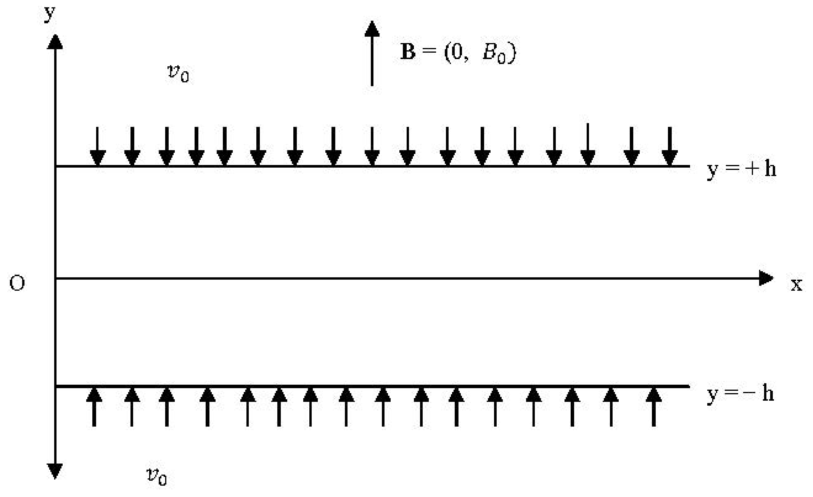
2. Formulation of the Problem

Here, a laminar incompressible micropolar fluid was considered along a two-dimensional permeable channel with porous walls through which fluid was uniformly injected or removed with velocity v 0 . The walls of the channel were taken to be parallel to x-axis at 2 h distance apart with lower boundary y = −h; upper y = h; and y-axis taken perpendicular to the walls. The lower channel wall was maintained at temperature T 1 and solute concentration C 1 , while the upper wall was maintained with temperature T 2 and solute concentration C 2 . A uniform magnetic field B was applied perpendicular to the channel walls. (Figure 1).
Following [25,26], the governing equations of the problem are
u x + v y = 0
ρ u u x + v u y = P x + ( μ + κ ) 2 u x 2 + 2 u y 2 + κ N y σ B 0 2 u
ρ u N x + v N y = κ j 2 N + u y v x + ν s j 2 N x 2 + 2 N y 2
ρ u v x + v v y = P y + ( μ + κ ) 2 v x 2 + 2 v y 2 κ N x
ρ u T x + v T y = K 1 C p 2 T y 2 1 C p q r y
ρ u C x + v C y = D * 2 C y 2
where u and v denote the velocity components along x-axis and y-axis directions, respectively, and ρ is the fluid density, μ is the dynamic viscosity, κ is the material parameter, N is the microrotation velocity, P is the fluid pressure and T, C and C p are the fluid temperature, species concentration and specific heat at constant pressure, respectively, K 1 is the thermal conductivity, D * is the molecular diffusivity, j is the micro-inertia density, v s = μ + κ 2 j is the microrotation viscosity and q r is the radiative heat flux.
The appropriate boundary conditions are
u = 0 , v = v 0 , N = s u y , T = T 1 , C = C 1   at   y = h
u = u 0 x h , v = v 0 , N = s u y , T 1 = T 2 , C = C 2 at   y = + h
where s denotes the boundary parameter representing the degree to which microelements are free to rotate near the channel walls. The case s = 0 means the strong concentration which shows that microelements are not rotating near the channel walls, s = 1 / 2 shows the weak concentrations and vanishing of the anti-symmetric part of the stress tensor, whereas s = 1 represents turbulent flow [26]. We introduced the following non-dimensional similarity variables in the case of strong concentration as:
η = y h , ψ = v 0 x f ( η ) , N = v 0 x h 2 g ( η ) , θ ( η ) = T T 1 T 2 T 1 ,   ϕ ( η ) = C C 1 C 2 C 1
where, T 2 = T 1 + A x , C 2 = C 1 + B x with A and B as constants [26]. The velocity components of flow are defined by stream function as u = ψ y , v = ψ x .
Using Similarity Transformations (9), Equations (2)–(4), after eliminating, p become
( 1 + N 1 ) f v N 1 g R e ( f f f f ) M f = 0
N 2 g + N 1 ( f 2 g ) N 3 R e ( f g f g ) = 0
Using Roseland approximation, we have q r = 4 σ 0 3 k 0 T 4 y where σ 0 the Stefan Boltzmann constant is and k 0 is the mean absorption coefficient. Assuming that the difference in temperature within the flow is such that T 4 can be expressed as linear combination of the temperature. Therefore expanding T 4 about T and ignoring higher order terms, we have T 4 3 T 4 + 4 T 3 T
q r = 4 σ 0 3 k 0 y 3 T 4 + 4 T 3 T = 16 σ 0 T 3 3 k 0 T y , q r y = 16 σ 0 T 3 3 k 0 A x h 2 θ ( η )
Using Similarity Transformations (9) and Equation (12), Equations (5) and (6) lead to
θ + P e h 1 + 4 3 N r f θ f θ = 0
ϕ + P e m f ϕ f ϕ = 0
With Boundary Conditions
f ( 1 ) = 0 , f ( 1 ) = 1 , g ( 1 ) = 0 ,   θ ( 1 ) = 0 ,   ϕ ( 1 ) = 0
f ( 1 ) = 1 , f ( 1 ) = 1 ,   g ( 1 ) = 1 , θ ( 1 ) = 1 , ϕ ( 1 ) = 1
where N 1 = κ μ is the micro-polar parameter, M = σ B 0 2 h 2 μ is the Magnetic parameter, N 2 = ν s μ h 2 is the spin gradient viscosity parameter, N 3 = j h 2 , N r = 4 σ 0 T 3 κ 1 κ 0 is the Radiation parameter, P r = ν ρ C p κ 1 is the Prandtl number. R e = v 0 h ν is the Reynolds number [for suction R e > 0 , for injection R e < 0 ], P e h = P r R e is the Peclet number for diffusion of heat, P e m = S c R e is the Peclet number for diffusion of mass and S c = ν D * is the generalized Schmidt number.
The physical quantities which are of greatest interest are local Sherwood number and local Nusselt number which are defined as follows:
S h x = 1
N u x = ( 1 + 4 N r 3 ) θ ( 1 )

3. Analysis of the Homotopy Perturbation Method (HPM)

The basic idea of HPM is illustrated in [27]. Accordingly, we consider the following equation
A u f r = 0 , r Ω
with the boundary condition
B u ,   u n = 0 , r Γ ,
where A is a general differential operator, B a boundary operator, f(r) a known analytical function and Γ is the boundary of the domain Ω . According to the method, A is divided into two parts which are L and N, where, L is linear operator and N is nonlinear. Therefore, the Equation (19) can be rewritten as follows:
L u + N u f r = 0 , r Ω .
Now the homotopy perturbation structure is shown as follows:
H v , p 1 p L v L u 0 + p A v f r = 0
where,
v r , p : Ω × 0 , 1 R .
In the Equation (22), p 0 , 1 is an embedding parameter and u 0 is the first approximation that satisfies the boundary condition. We can assume that the solution of the Equation (23) can be written as a power series in p , as follows:
v = v 0 + p v 1 + p 2 v 2 +
and the best approximation for solution is given as
u = lim p 1 v = v 0 + v 1 + v 2 +

4. Solution of the Problem by HPM

In order to solve the nonlinear differential Equations (10), (11), (13) and (14) by HPM, we constructed a homotopy as follows:
H f , p = 1 p f i v f 0 i v + p 1 + N 1 f i v N 1 g R e f f f f M f = 0
H g , p = 1 p g g 0 + p N 2 g + N 1 f 2 g N 3 R e f g f g = 0
H θ , p = 1 p θ θ 0 + p 1 + 4 3 N r θ + p P e h f θ f θ = 0
H ϕ , p = 1 p ϕ ϕ 0 + p ϕ + P e m f ϕ f ϕ = 0
Now f ,   g ,   θ and ϕ can be explained as follows:
f = f 0 + p f 1 + p 2 f 2 +
g = g 0 + p g 1 + p 2 g 2 +
θ = θ 0 + p θ 1 + p 2 θ 2 +
ϕ = ϕ 0 + p ϕ 1 + p 2 ϕ 2 +
Substituting Equations (30)–(33) into Equations (26)–(29) and simplifying and re-arranging based on power of p -terms, we obtain:
for p 0 :
f 0 i v = 0 ,   g 0 = 0 ,   θ 0 = 0 ,   ϕ 0 = 0
and boundary conditions are:
η = 1   :   f 0 = 1 ,   f 0 = g 0 = θ 0 = ϕ 0 = 0 η = + 1   :   f 0 = g 0 = θ 0 = ϕ 0 = 1 ,   f 0 = 1
for p 1 :
( 1 + N 1 ) f 1 i v N 1 g 0 R e f 0 f 0 f 0 f 0 M f 0 = 0 N 2 g 1 + N 1 f 0 2 g 0 N 3 R e f 0 g 0 f 0 g 0 = 0 1 + 4 3 N r θ 1 + P e h f 0 θ 0 f 0 θ 0 = 0 ϕ 1 + P e m f 0 ϕ 0 f 0 ϕ 0 = 0
and boundary conditions are:
η = 1   :   f 1 = f 1 = g 1 = θ 1 = ϕ 1 = 0 η = + 1   :   f 1 = g 1 = θ 1 = ϕ 1 = f 1 = 0
Solving Equations (34) and (36) with boundary conditions, we have
f 0 η = 0.75 η 3 0.25 η 2 + 1.75 η + 0.25 g 0 = 0.5 η + 0.5 θ 0 = 0.5 η + 0.5 ϕ 0 = 0.5 η + 0.5
f 1 η = R e 1 + N 1 0.0080357143 η 7 0.00625 R e + M 1 + N 1 η 6 R e 1 + N 1 0.0020833333 + M 1 + N 1 0.0041666667 η 5 + R e 1 + N 1 0.0260416667 + M 1 + N 1 0.072916667 η 4 + R e 1 + N 1 0.360863095 M 1 + N 1 0.089453125 η 3 + R e 1 + N 1 0.360863095 M 1 + N 1 0.089453125 η 3 R e 1 + N 1 0.03333333334 + M 1 + N 1 0.209375 η 2 + M 1 + N 1 0.124609375 η + [ M 1 + N 1 0.11171875 R e 1 + N 1 0.041592261
g 1 η = N 3 R e N 2 0.375 η 5 + N 3 R e N 2 0.1041666667 η 4 + N 3 R e N 2 0.0416666667 + N 1 N 2 0.9166666667 η 3 + N 1 N 2 0.75 N 3 R e N 2 0.375 η 2 N 3 R e N 2 0.0761666667 + N 1 N 2 0.9166666667 η + N 3 R e N 2 0.2708333333 N 1 N 2 0.75
θ 1 η = P e h 1 + 4 3 N r 0.0375 η 5 + 0.1041666667 η 4 + 0.0416666667 η 3 0.375 η 2 P e h 1 + 4 3 N r 0.0791666667 η + P e h 1 + 4 3 N r 0.2708333333
ϕ 1 η = P e m 0.0375 η 5 + 0.1041666667 η 4 + 0.0416666667 η 3 0.375 η 2 P e m 0.0791666667 η + P e m 0.2708333333
The terms f i η , g i η , θ i η and ϕ i η for i 2 are too large to present graphically.
The solution of the Equations (30)–(33), where p = 1 will be as
f η = f 0 η + f 1 η + f 2 η + g η = g 0 η + g 1 η + g 2 η + θ η = θ 0 η + θ 1 η + θ 2 η + ϕ η = ϕ 0 η + ϕ 1 η + ϕ 2 η +

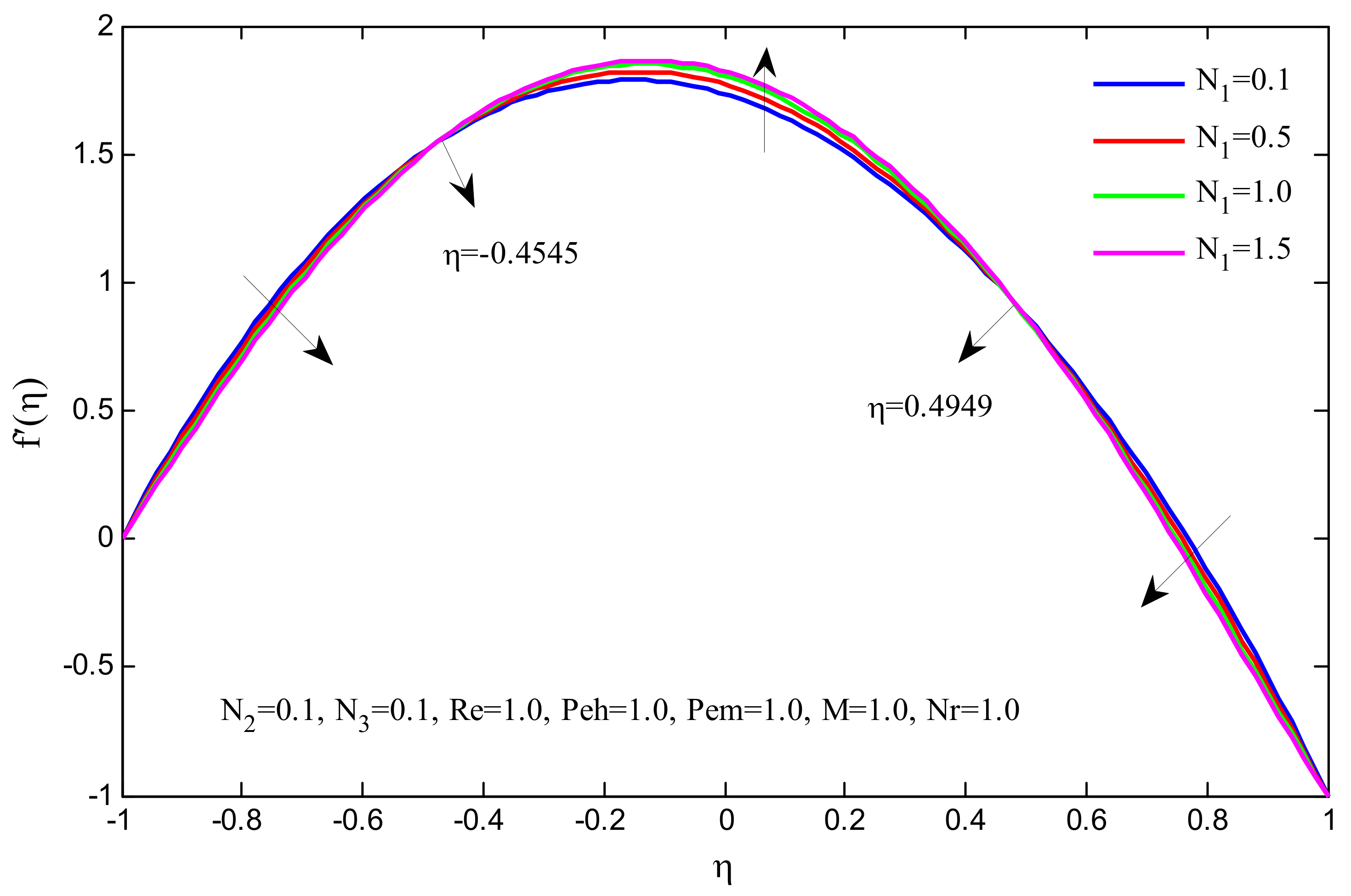
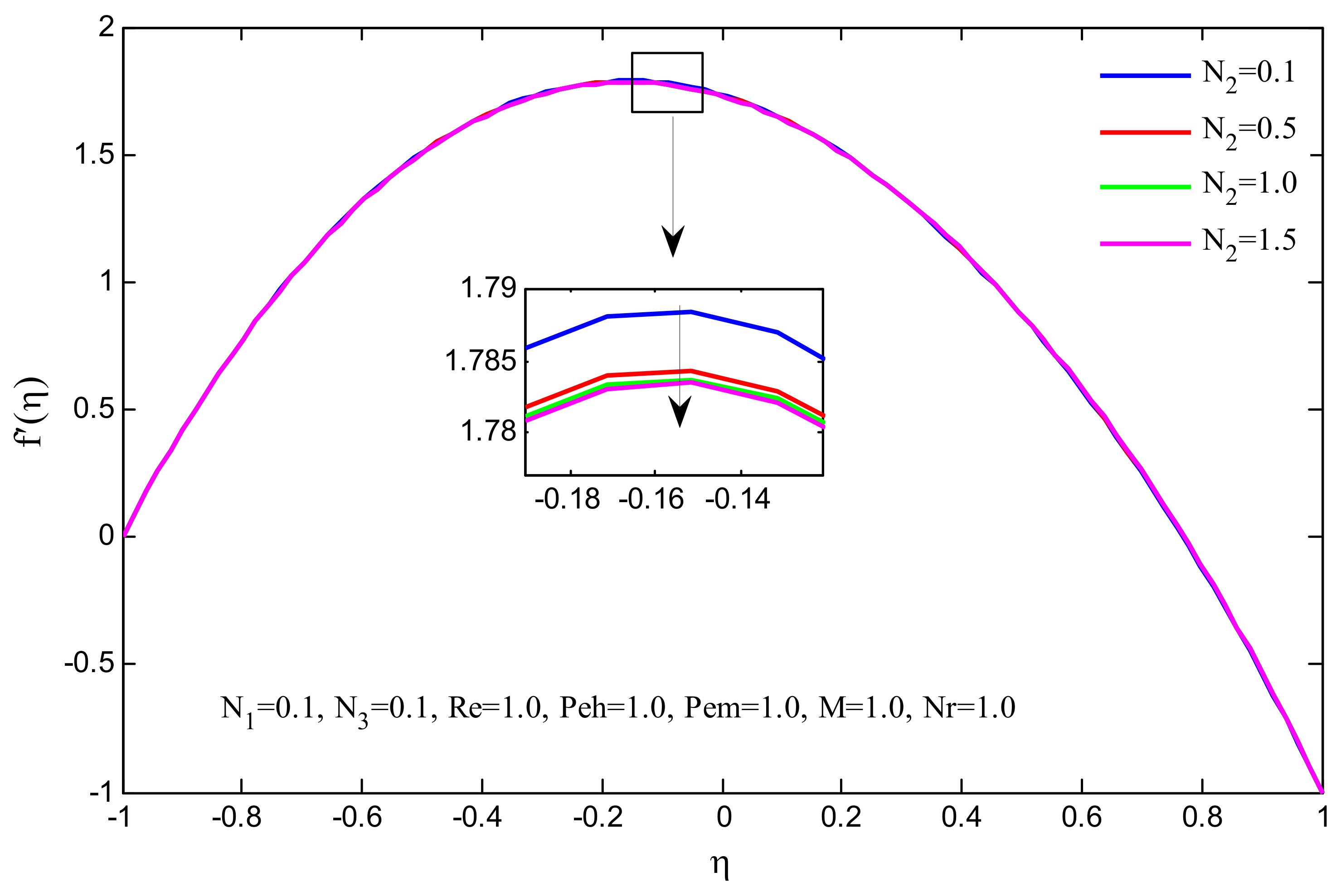
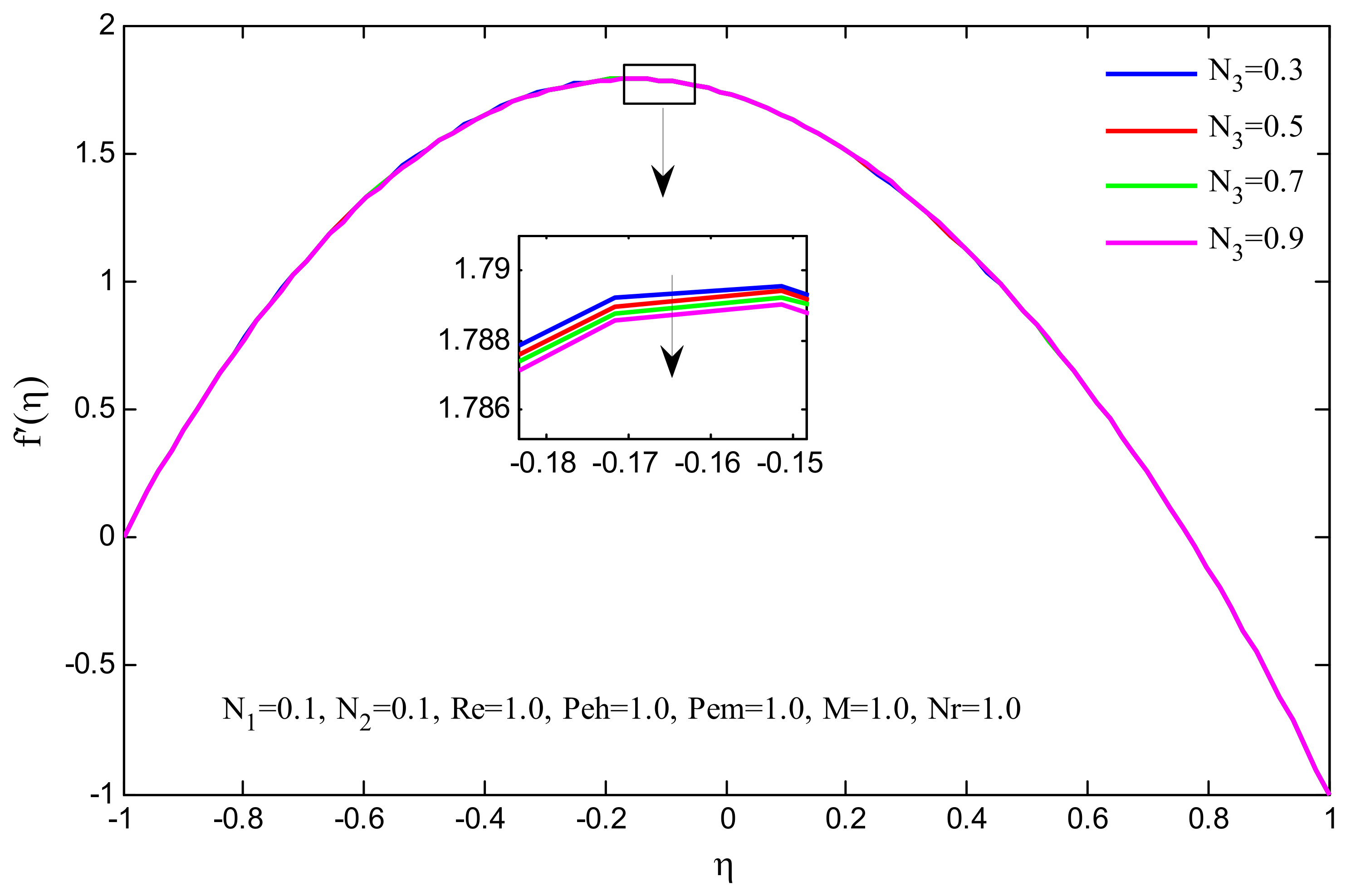
5. Results and Discussions

The transformed Equations (10), (11), (13) and (14) along with the boundary conditions (15) and (16) were solved numerically by the bvp4c routine in MATLAB and the results thus obtained were developed into graphs in which the behaviour of non-dimensional parameters like N 1 ,   N 2 ,   N 2 ,   R e ,   P e h ,   P e m etc. on the simulated fluid velocity, microrotation profile and temperature profiles are shown through Figure 2, Figure 3, Figure 4, Figure 5, Figure 6, Figure 7, Figure 8, Figure 9, Figure 10, Figure 11, Figure 12 and Figure 13.
Figure 2, Figure 3 and Figure 4 depicts the effect of N1, N2 and N3 respectively on simulated velocity. As in Figure 2 when η < −0.4545 velocity decreases and after that it start increasing and as η > 0.4949 it again decreases. That is, N 1 has a dual effect on simulated velocity while on increasing N 2 and N 3 , the simulated velocity decreases (see Figure 3 and Figure 4).
It can be seen in Figure 5 that keeping the other parameters fixed, when η < −0.6566 velocity decreases for R e < 2.0 and an increase in velocity is shown for R e > 2.0 , it starts decreasing when 0.6566 < η < 0.3535 and it start increasing when η > 0.3535. As the Reynolds number increases, the fluid velocity decreases in the middle of the channel, whereas near the lower wall of the channel it decreases when the Reynolds number remains below 2.0; it starts increasing when the Reynolds number is above 2.0, but near the upper wall of the channel, it appears to increase when the Reynolds number increases from 1.0 to 4.0.
Figure 6 portrays the effect of the magnetic field on simulated velocity. It increases as M increases, but after reaching η = −0.05051, the velocity decreases. In the presence of the magnetic field, the fluid oscillates irregularly in the middle of the channel.
Figure 7 shows that the micro-elements of the fluid irregularly oscillate around the middle of the channel as N 1 increases. As the coupling parameter gradually increases, it is reflectedby the irregular oscillation of micro-elements around the middle of the channel.
Figure 8 shows that with an increase in N2, micro-elements irregularly oscillate around η < −0.5, that is, due to the increase of spin gradient viscosity, micro-elements oscillate in an irregular mode near the lower wall of the channel.
An increase in N3 leads to the irregular oscillation of micro-elements around η < −0.3, that is, the micro-elements oscillate near the lower wall of the channel as N3 increases (Figure 9).
Figure 10 demonstrates that the micro-elements irregularly oscillate near the lower wall of the channel at around (−0.6, −0.4) as Reynolds number increases.
Figure 11 shows that the increase in the value of Nr leads to a decrease in the temperature field and that the maximum decrease in temperature is at the middle of the channel, indicating that larger the radiation parameter lower the temperature in the middle of the channel.
In Figure 12, it can be observed that the fluid temperature increases in the middle of the channel when P e h = 0.5 to P e h = 1.5 , and the temperature rapidly increases when P e h = 1.5 onwards.
Figure 13 shows the effect of Peclet number for the diffusion of mass in a concentration profile. The solute concentration will be at a maximum in the middle of the channel as the diffusion of mass increases but it remains non-zero at the upper wall of the channel.

6. Conclusions

The micropolar parameter N 1 has a dual effect on simulated velocity while the spin gradient viscosity parameter N 2 and N 3 both have an adverse effect on simulated velocity.
On increasing N 1 , the microrotation irregularly oscillates around the middle of the channel, whereas on increasing spin gradient viscosity N2, micro-elements irregularly oscillate around η < −0.5;an increase in N3 leads to irregular oscillation at an angular velocity around η < −0.3.
The Reynolds number impacts dual effect on simulated velocity about R e = 2.0 when 1 < η < 0.6566 and increasing the Reynolds number leads to irregular oscillations in microrotation.
The simulated velocity irregularly oscillates around η = −0.05051, when M increases.
Nr plays a key role in decreases in the temperature profile and the maximum fall in temperature is noticed near middle of the channel.
The fluid temperature increases in the middle of the channel when P e h = 0.5 to P e h = 1.5 and the temperature rapidly increases when P e h = 1.5 onwards; the upper wall of the channel will experience increases in temperature but the lower wall will have negligible increases in temperature.
Peclet number Pem for diffusion of mass indicates that mass diffusion will be at a maximum in the middle of the channel.
From Table 1, it has been observed that local heat flux increases when M < 10 and starts decreasing when M > 10, and inversely depends on Reynolds number. Its dependence on N 2 and N 3 is inverse, while on N 1 it is directly proportional. The heat flux increases when the values of Peh increase, whereas it decreases when increasing the values of radiation parameter N r .
Table 1 also predicts that the mass flux depends only on P e m and it starts increasing upon increasing P e m .

7. Comparison of This Work with Other Work

In the absence of the magnetic field and thermal radiation, the Equations (10), (13) and (14) reduce equations obtained by M. Sheikholeslami et al. [24], but we have taken different boundary conditions in our paper. If we take the same boundary conditions as taken by [24], then the graphical representation of microrotation in our Figure 7, Figure 8, Figure 9 and Figure 10 will be reduced to the same as is shown in [24]. In the absence of the magnetic field and thermal radiation, the governing equations of our problem have been reduced to the governing equations as in A. Mirzaaghaian et al. [25], and if we take the boundary conditions to be the same as in [25], the graphical representation of the temperature profile matches with Figure 11 and Figure 12 in our paper. Thus, in the presence of the magnetic field and thermal radiation, we have obtained the new results presented in the Results and Discussion section of this study.

Author Contributions

V.A. and B.S.; Formal analysis, W.J., A.H.A. and H.Y.Z.; Investigation, V.A., A.K., K.S.N. and W.J.; Software, V.A., B.S., A.K. and K.S.N.; Validation, B.S. and W.J.; Writing–original draft, V.A., B.S., A.K., K.S.N. and W.J.; Writing review and Editing: V.A., B.S., K.S.N., A.H.A. and H.Y.Z.; Funding acquisition: A.H.A. and H.Y.Z.; All authors have read and agreed to the published version of the manuscript.

Funding

This work received finding from King Khalid University Ministry of Education, and Taif University Saudi Arabia.

Institutional Review Board Statement

Not applicable.

Informed Consent Statement

Not applicable.

Data Availability Statement

Not applicable.

Acknowledgments

The authors express their appreciation to the Deanship of Scientific Research at King Khalid University for funding this work through the research groups program under grant number R.G.P.2/111/41. The authors extend their appreciation to the Deputyship for Research & Innovation, Ministry of Education, in Saudi Arabia for funding this research work through the project number: (IFP-KKU-2020/9). The authors would like to acknowledge financial support from the Taif University Researchers Supporting Project number TURSP-2020/252, Taif University, Taif, Saudi Arabia. The authors gratefully thank to the referees for the constructive comments and recommendations which help to improve the readability and quality of the paper.

Conflicts of Interest

The authors declare no conflict of interest.

Nomenclature

Cspecies concentration
D*molecular diffusivity
K 1 thermal conductivity
B 0 strength of constant applied magnetic field
dimensionless stream function
gdimensionless microrotation
hhalf width of channel
jmicro-inertia density
Mmagnetic parameter
Nmicrorotation/angular velocity
N1, 2, 3dimensionless parameters
N u x Local Nusselt number
S u x Local Sherwood number
ScSchmidt number
Ppressure
PrPrandtl number
P e h Peclet number for diffusion of heat
P e m Peclet number for diffusion of mass
q r radiative heat flux
ReReynolds number
Tfluid temperature
Nrradiation parameter
smicrorotation boundary condition
(u, v)Cartesian velocity components
(x, y)Cartesian coordinate components parallel & normal to channel axis, respectively
HPMhomotopy perturbation method

Greek Symbols

ηsimilarity variable
μdynamic viscosity
ρFluid density
ψ stream function
σ electric conductivity
θdimensionless temperature
ϕ dimensionless mass transfer parameter
κcoupling coefficient
ν s microrotation/spin-gradient viscosity

References

  1. Abo-Eldahab, E.M.; Ghonaim, A.F. Radiation effect on heat transfer of a micropolar fluid through a porous medium. Appl. Math. Comput. 2005, 169, 500–510. [Google Scholar] [CrossRef]
  2. Perdikis, C.; Raptis, A. Heat transfer of a micropolar fluid by the presence of radiation. Heat Mass Transf. 1996, 31, 381–382. [Google Scholar] [CrossRef]
  3. Raptis, A. Flow of a micropolar fluid past a continuously moving plate by the presence of radiation. Int. J. Heat Mass Transf. 1998, 41, 2865–2866. [Google Scholar] [CrossRef]
  4. Seddeek, M.; Abdelmeguid, M. Effects of radiation and thermal diffusivity on heat transfer over a stretching surface with variable heat flux. Phys. Lett. A 2006, 348, 172–179. [Google Scholar] [CrossRef]
  5. El-Arabawy, H.A. Effect of suction/injection on the flow of a micropolar fluid past a continuously moving plate in the presence of radiation. Int. J. Heat Mass Transf. 2003, 46, 1471–1477. [Google Scholar] [CrossRef]
  6. Sharma, R.; Gupta, U. Thermal convection in micropolar fluids in porous medium. Int. J. Eng. Sci. 1995, 33, 1887–1892. [Google Scholar] [CrossRef]
  7. Ramachandran, P.; Mathur, M.; Ojha, S. Heat transfer in boundary layer flow of a micropolar fluid past a curved surface with suction and injection. Int. J. Eng. Sci. 1979, 17, 625–639. [Google Scholar] [CrossRef]
  8. Takhar, H.; Bhargava, R.; Agrawal, R.; Balaji, A. Finite element solution of micropolar fluid flow and heat transfer between two porous discs. Int. J. Eng. Sci. 2000, 38, 1907–1922. [Google Scholar] [CrossRef]
  9. Kelson, N.; Farrell, T. Micropolar flow over a porous stretching sheet with strong suction or injection. Int. Commun. Heat Mass Transf. 2001, 28, 479–488. [Google Scholar] [CrossRef]
  10. Ashraf, M.; Kamal, M.A.; Syed, K. Numerical study of asymmetric laminar flow of micropolar fluids in a porous channel. Comput. Fluids 2009, 38, 1895–1902. [Google Scholar] [CrossRef]
  11. Majdalani, J.; Zhou, C.; Dawson, C.A. Two-dimensional viscous flow between slowly expanding or contracting walls with weak permeability. J. Biomech. 2002, 35, 1399–1403. [Google Scholar] [CrossRef]
  12. Terrill, R.M.; Shrestha, G.M. Laminar flow through parallel and uniformly porous walls of different permeability. Z. Angew. Math. Phys. 1965, 16, 470–482. [Google Scholar] [CrossRef]
  13. Asghar, S.; Mushtaq, M.; Hayat, T. Flow in a slowly deforming channel with weak permeability: An analytical approach. Nonlinear Anal. Real World Appl. 2010, 11, 555–561. [Google Scholar] [CrossRef]
  14. He, J.-H. Homotopy perturbation method for solving boundary value problems. Phys. Lett. A 2006, 350, 87–88. [Google Scholar] [CrossRef]
  15. He, J.-H. Homotopy perturbation method for bifurcation of nonlinear problems. Int. J. Nonlinear Sci. Numer. Simul. 2005, 6, 207–208. [Google Scholar] [CrossRef]
  16. Ganji, D.D. The application of he’s homotopy perturbation method to nonlinear equations arising in heat transfer. Phys. Lett. A 2006, 355, 337–341. [Google Scholar] [CrossRef]
  17. Biazar, J.; Estami, M.; Ghazvini, H. Homotopy Perturbation Method for Systems of Partial Differential Equations. Int. J. Nonlinear Sci. Numer. Simul. 2007, 8, 411–416. [Google Scholar] [CrossRef]
  18. Fereidoon, A.; Ganji, D.D.; Rostamiyan, Y. Application of he’s homotopy perturbation and variational iteration methods to solving propagation of thermal stresses equation in an infinite elastic slab. Adv. Theor. Appl. Mech. 2008, 1, 199–215. [Google Scholar]
  19. Hemeda, A.A. Homotopy perturbation method for solving systems of nonlinear coupled equations. Appl. Math. Sci. 2012, 6, 4787–4800. [Google Scholar]
  20. Aminikhah, H.; Hemmatnezhad, M. A novel effective approach for solving nonlinear heat transfer equations. Heat Transf.-Asian Res. 2012, 41, 459–467. [Google Scholar] [CrossRef]
  21. Soltania, D.; Khorshidib, M.A. Application of homotopy perturbation and reconstruction of variational iteration methods for harry dym equation and compared with exact solution. Int. J. Multidiscip. Curr. Res. 2013, 1, 166–169. [Google Scholar]
  22. Yıldırım, A.; Kelleci, A. Homotopy perturbation method for numerical solutions of coupled Burger’s equations with time-and space-fractional derivatives. Int. J. Numer. Methods Heat Fluid Flow 2010, 20, 897–909. [Google Scholar] [CrossRef]
  23. Sheikholeslami, M.; Ganji, D.D.G.-D. Heat transfer of Cu-water nanofluid flow between parallel plates. Powder Technol. 2013, 235, 873–879. [Google Scholar] [CrossRef]
  24. Sheikholeslami, M.; Rokni, H.B.; Damiri-Ganji, D. Nanofluid flow in a semi-porous channel in the presence of uniform magnetic field. Int. J. Eng. 2013, 26, 653–662. [Google Scholar] [CrossRef]
  25. Sheikholeslami, M.; Hatami, M.; Ganji, D.D.G.-D. Micropolar fluid flow and heat transfer in a permeable channel using analytical method. J. Mol. Liq. 2014, 194, 30–36. [Google Scholar] [CrossRef]
  26. Mirzaaghaian, A.; Ganji, D. Application of differential transformation method in micropolar fluid flow and heat transfer through permeable walls. Alex. Eng. J. 2016, 55, 2183–2191. [Google Scholar] [CrossRef] [Green Version]
  27. He, J.H. Homotopy perturbation technique. Comput. Methods Appl. Mech. Eng. 1999, 178, 257–262. [Google Scholar] [CrossRef]
  28. Sibanda, P.; Awad, F. Flow of a micropolar fluid in channel with heat and mass transfer. In Proceedings of the 2010 International Conference on Theoretical and Applied Mechanics, International Conference on Fluid Mechanics and Heat & Mass Transfer, Corfu Island, Greece, 22–24 July 2010; pp. 112–120. [Google Scholar]
  29. Mirgolbabaee, H.; Ledari, S.; Ganji, D. Semi-analytical investigation on micropolar fluid flow and heat transfer in a permeable channel using AGM. J. Assoc. Arab. Univ. Basic Appl. Sci. 2017, 24, 213–222. [Google Scholar] [CrossRef] [Green Version]
  30. Singh, B. Thermal convection of MHD micropolar fluid layer heated from below saturating a porous medium. IOSR J. Eng. (IOSR-JEN) 2018, 8, 45–52. [Google Scholar]
  31. Singh, B. Hall effect on MHD flow of visco-elastic micro-polar fluid layer heated from below saturating a porous medium. Int. J. Eng. Sci. Technol. 2017, 9, 48–66. [Google Scholar] [CrossRef] [Green Version]
  32. Singh, B. Thermal instability of a rotating MHD micropolar fluid layer heated from below saturating a porous medium. Int. J. Pure Appl. Math. 2018, 118, 1393–1405. [Google Scholar]
  33. Mohammed, H.I.; Talebizadehsardari, P.; Mahdi, J.M.; Arshad, A.; Sciacovelli, A.; Giddings, D. Improved melting of latent heat storage via porous medium and uniform Joule heat generation. J. Energy Storage 2020, 31, 101747. [Google Scholar] [CrossRef]
  34. Ghaneifar, M.; Arasteh, H.; Mashayekhi, R.; Rahbari, A.; Mahani, R.B.; Talebizadehsardari, P. Thermohydraulic analysis of hybrid nanofluid in a multilayered copper foam heat sink employing local thermal non-equilibrium condition: Optimization of layers thickness. Appl. Therm. Eng. 2020, 181, 115961. [Google Scholar] [CrossRef]
  35. Ghalambaz, M.; Zadeh, S.M.H.; Mehryan, S.; Pop, I.; Wen, D. Analysis of melting behavior of PCMs in a cavity subject to a non-uniform magnetic field using a moving grid technique. Appl. Math. Model. 2020, 77, 1936–1953. [Google Scholar] [CrossRef]
  36. Ali, F.H.; Hamzah, H.K.; Hussein, A.K.; Jabbar, M.Y.; Talebizadehsardari, P. MHD mixed convection due to a rotating circular cylinder in a trapezoidal enclosure filled with a nanofluid saturated with a porous media. Int. J. Mech. Sci. 2020, 181, 105688. [Google Scholar] [CrossRef]
  37. Ghalambaz, M.; Groşan, T.; Pop, I. Mixed convection boundary layer flow and heat transfer over a vertical plate embedded in a porous medium filled with a suspension of nano-encapsulated phase change materials. J. Mol. Liq. 2019, 293, 34. [Google Scholar] [CrossRef]
Figure 1. Geometrical view of the problem.
Coatings 12 00011 g001
Figure 2. Effect of N 1 on simulated velocity.
Coatings 12 00011 g002
Figure 3. Effect of N 2 on simulated velocity.
Coatings 12 00011 g003
Figure 4. Effect of N3 on simulated velocity.
Coatings 12 00011 g004
Figure 5. Effect of Re on simulated velocity.
Coatings 12 00011 g005
Figure 6. Effect of M on simulated velocity.
Coatings 12 00011 g006
Figure 7. Effect of N1 on microrotation profile.
Coatings 12 00011 g007
Figure 8. Effect of N2 on microrotation profile.
Coatings 12 00011 g008
Figure 9. Effect of N3 on microrotation profile.
Coatings 12 00011 g009
Figure 10. Effect of Re on microrotation profile.
Coatings 12 00011 g010
Figure 11. Effect of Nr on temperature profile.
Coatings 12 00011 g011
Figure 12. Effect of P e h on temperature profile.
Coatings 12 00011 g012
Figure 13. Effect of P e m on mass concentration profile.
Coatings 12 00011 g013
Table 1. Numerical values of −θ′(−1) and −φ′(−1) for different values of N 1 ,   N 2 ,   N 3 ,   R e ,   M   P e h ,   P e m and   N r .
N1N2N3ReM P e h P e m Nrθ′(−1)
1.01.01.01.01.00.10.10.10.5535
1.01.01.01.03.00.10.10.10.5536
1.01.01.01.05.00.10.10.10.5537
1.01.01.01.010.00.10.10.10.5537
1.01.01.01.015.00.10.10.10.5536
1.01.01.01.020.00.10.10.10.5535
1.01.01.03.01.00.10.10.10.5552
1.01.01.05.01.00.10.10.10.5538
1.01.01.010.01.00.10.10.10.5532
1.01.01.51.01.00.10.10.10.5532
1.01.01.61.01.00.10.10.10.5530
1.01.02.01.01.00.10.10.10.5520
1.01.5 1.01.01.00.10.10.10.5533
1.01.61.01.01.00.10.10.10.5532
1.02.01.01.01.00.10.10.10.5530
1.51.01.01.01.00.10.10.10.5537
1.61.01.01.01.00.10.10.10.5538
2.01.01.01.01.00.10.10.10.5539
1.01.01.01.01.00.20.10.10.6167
1.01.01.01.01.00.30.10.10.6922
1.01.01.01.01.00.40.10.10.7842
1.01.01.01.01.00.10.10.20.5475
1.01.01.01.01.00.10.10.30.5427
1.01.01.01.01.00.10.10.40.5387
N1N2N3ReM P e h P e m Nrφ′(−1)
1.01.01.01.01.00.10.1 0.10.5613
1.01.01.01.01.00.10.20.10.6355
1.01.01.01.01.00.10.30.10.7268
1.01.01.01.01.00.10.40.10.8420
Publisher’s Note: MDPI stays neutral with regard to jurisdictional claims in published maps and institutional affiliations.

