Article

MHD Hybrid Nanofluid Flow Due to Rotating Disk with Heat Absorption and Thermal Slip Effects: An Application of Intelligent Computing

by
Muhammad Shoaib
1,
Muhammad Asif Zahoor Raja
2,*,
Muhammad Touseef Sabir
1,
Kottakkaran Sooppy Nisar
3,*,
Wasim Jamshed
4,
Bassem F. Felemban
5 and
I. S. Yahia
6,7,8
1
Department of Mathematics, Attock Campus, COMSATS University Islamabad, Islamabad 64002, Pakistan
2
Future Technology Research Center, National Yunlin University of Science and Technology, 123 University Road, Section 3, Yunlin, Douliou 64002, Taiwan
3
Department of Mathematics, College of Arts and Science, Prince Sattam bin Abdulaziz University, Wadi Aldawaser 11991, Saudi Arabia
4
Department of Mathematics, Capital University of Science and Technology (CUST), Islamabad 44000, Pakistan
5
Department of Mechanical Engineering, College of Engineering, Taif University, P.O. Box 11099, Taif 21944, Saudi Arabia
6
Laboratory of Nano-Smart Materials for Science and Technology (LNSMST), Department of Physics, Faculty of Science, King Khalid University, P.O. Box 9004, Abha 61413, Saudi Arabia
7
Research Center for Advanced Materials Science (RCAMS), King Khalid University, P.O. Box 9004, Abha 61413, Saudi Arabia
8
Nanoscience Laboratory for Environmental and Biomedical Applications (NLEBA), Semiconductor Lab, Department of Physics, Faculty of Education, Ain Shams University, Roxy, Cairo 11757, Egypt
*
Authors to whom correspondence should be addressed.
Coatings 2021, 11(12), 1554; https://doi.org/10.3390/coatings11121554
Submission received: 22 November 2021 / Revised: 10 December 2021 / Accepted: 13 December 2021 / Published: 17 December 2021
(This article belongs to the Special Issue Nanofluidics: Interfacial Transport Phenomena)

Abstract

:
The objective of this study is to explore the flow features and heat transfer properties of an MHD hybrid nanofluid between two parallel plates under the effects of joule heating and heat absorption/generation (MHD-HFRHT) by utilizing the computational strength of Levenberg–Marquardt Supervised Neural Networks (LM-SNNs). Similarity equations are utilized to reduce the governing PDEs into non-linear ODEs. A reference solution in the form of data sets for MHD-HFRHT flow is obtained by creating different scenarios by varying involved governing parameters such as the Hartman number, rotation parameter, Reynolds number, velocity slip parameter, thermal slip parameter and Prandtl number. These reference data sets for all scenarios are placed for training, validation and testing through LM-SNNs and the obtained results are then compared with reference output to validate the accuracy of the proposed solution methodology. AI-based computational strength with the applicability of LM-SNNs provides an accurate and reliable source for the analysis of the presented fluid-flow system, which has been tested and incorporated for the first time. The stability, performance and convergence of the proposed solution methodology are validated through the numerical and graphical results presented, based on mean square error, error histogram, regression plots and an error-correlation measurement. MSE values of up to the accuracy level of 1 × 10⁻¹¹ established the worth and reliability of the computational technique. Due to an increase in the Hartmann number, a resistance was observed, resulting in a reduction in the velocity profile. This occurs as the Hartmann number measures the relative implication of drag force that derives from magnetic induction of the velocity of the fluid flow system. However, the Reynolds number accelerates in the velocity profile due to the dominating impact of inertial force.

1. Introduction

Nowadays, the rapid developments in the field of science and technology demands for more compact and smart devices in terms of better performance, long life and precise operation. For this purpose, many efforts have been made in recent decades to improve the rate of heat transfer of various fluids to achieve better thermal and physical properties. Conventional ways of improving the heat transfer rate through a proper variation of the velocity field without consuming energy have gained much attention. Thermal conductivity plays an important and vital role among all other properties in judging the heat transfer abilities of the fluid. Ultimately, the improvement of the heat-transfer rate in a fluid by improving the thermos physical properties with the addition of nanoparticles was an innovative work. Many efforts have been made to enhance the thermal abilities of conventional fluids with the addition of metallic and non-metallic nano-particles of sizes less than 100 nm. The field of heat transfer was revolutionized by Choi [1] in 1995, when he introduced a new class of fluid known as “nanofluid”, with excellent thermal transport properties as compared to conventional fluids. King et al. [2] verified and validated the theoretical results of Choi. Afterward, Lee et al. [3] experimentally calculated the rate of heat transfer for nanofluids consisting of Cu and Al2O3nanoparticles. Even though, these nanofluidic system fulfill many of the industrial and engineering requirements, researchers are still in search of more efficient nanofluidic systems.
In the recent years, many studies have been carried out using next generation hybrid or mixed nanofluid, which are prepared by dispersing two or more types of nanoparticles in a base fluid. The basic purpose of the hybrid nanofluid is to enhance the heat transfer properties as compared to based fluid, due to the synergetic effects of various kinds of nanomaterials. Due to their marvelous heat transfer abilities, hybrid nanofluids have an extensive application range in industrial, engineering and medical fields such as in a HVAC system, micro channel heat sink (MCHS), solar heating systems, transformer cooling, electronic cooling, biomedical and food processing [4]. In recent years, many researchers have explored the flow behavior of hybrid nanofluid in various geometries and compared the performance along with heat transfer ability of hybrid nanofluid with conventional base fluids [5,6,7,8].
Shoaib et al. [9] investigated the flow properties and heat transfer effects in 3D MHD flow of a water-based hybrid nanofluid over an extendable sheet under the influence of thermal radiation. Furthermore, the behavior of velocity and the temperature field were also examined against various physical constraints. Rajesh et al. [10] numerically compared the results of heat and mass transfer for CuO-Ag/H2O (Hybrid nanofluid) and CuO/H2O (nanofluid) over a vibrating cylindrical chamber. Devi et al. [11] discussed the boost in the rate of transfer rate by using the hybrid nanofluid in a three dimensional stretchable surface with MHD and Newton heating effects. Nagoor et al. [12] used a bvp4c solution technique to investigate the flow of hybrid nanofluid in a revolving frame under thermal radiation effects. Alempour et al. [13] studied the flow inside a 3-D elliptical tube with circular cross section. The results obtained revealed an increment in heat transfer and increased of friction has been observed by transforming the cross section of tube from a circular to elliptical shape. Ouyang et al. [14] examined the influence of different constraints on the flow of 3D hybrid nanofluid over a rotating disk with uniform magnetic field.
Waini et al. [15] used a bvp4c solver to numerically study the transpiration effects over the flow and rate of heat transfer over a stretchable sheet inside a uniform flow of hybrid nanofluid. Afridi et al. [16] performed a comparative numerical analysis of entropy generation between ordinary nanofluid and hybrid nanofluid. A reduction in entropy generation was observed with an increase in the velocity of a fluid. Furthermore, the influence of various physical constraints over velocity, temperature and entropy generation has been studied. Shafiq et al. [17] utilized response surface methodology (RSM) to study the thermo-bio-convective flow over a stretching/shrinking surface with the effects of Brownian motion and thermophoresis. Nadeem et al. [18] numerically evaluated the heat transfer rate in the flow of a hybrid nanofluid over a stretching and porous surface as compared to ordinary nanofluid. Anuar et al. [19] presented a stability analysis for the flow of a hybrid nanofluid with injection/suction and thermal radiation effects over a rotating stretchable sheet. Sreedevi et al. [20] analyzed the heat and mass transfer in MHD flow of MWCNT-Ag/H2O hybrid nanofluid with suction, chemical reaction, slip and thermal radiation effects. Venkateswarlu et al. [21] discussed the impact of variable viscosity along with viscous dissipation on the flow of Cu-Al2O3/H2O hybrid fluid with radiative heating. Ahmed et al. [22] and Kandasamy et al. [23] investigated the effects of the shape factor of nanoparticles on time-dependent MHD squeezed flow between two parallel plates while considering the phenomenon of viscous dissipation. The influence of several physical parameters on the velocity and temperature field has also been analyzed numerically. Shoaib et al. [24] compared the behavior of different physical constraint on mass as well as heat transfer for a three dimensional flow of hybrid nanofluid over a revolving plane under thermal radiation and viscous dissipation effects. Xiang and Mujumdar [25] examined the suspensions of nanometer-sized particles in based fluids under the impacts of connective thermal energy system.
Non-Newtonian fluids are those fluids for which the proper relationship between stress and strain rate is disrupted. Non-Newtonian fluids are used in the lubricants, detergents, paints, plastic and nylons industries. Stress inside the viscoelastic fluid is not instantly eliminated through the removal of applied stress due to the intermolecular structure. This unique property of non-Newtonian fluid is termed as the memory effect. The non-Newtonian fluid model provided by Reiner [26] and Rivlin [27] presented a non-Newtonian fluid model to predict flow behaviors of various biological products as well as many food products and polymers. The authors discussed that nanofluids, involving suspended particles, help in the modifications of the transport properties. Moreover, a theoretical as well as numerical study of a variety of applications and thermal properties of nanofluid are provided in detail. Elahi et al. [28,29] studied the nanofluid-flow dynamics in the presence of hafnium particles past slippery wall. Moreover, the authors analyzed the impacts of heat transfer and magneto hydrodynamics during the entropy generation system. Almarit et al. [30] investigated the impacts of MHD and mass transfer using the Cattaneo-Christove heat flux system.
Many of the researchers used traditional deterministic techniques to solve various fluid dynamics problems including Joule heating, entropy generation, nanofluid and viscous dissipation [31,32,33,34], Molecular Sensitivity of Near-Field Vibrational Infrared Imaging [35], Capillary driven flow in nanochannels [36], application of MnO2-Fe3O4/CuO hybrid catalysts [37] and Molecule-Plasmon Excitation Coupling [38], and the solution of such problems through modern stochastic solution methods based on the artificial intelligence algorithm is innovative. Stochastic solution techniques based on artificial intelligence (AI) algorithms are better and efficient alternatives for various linear and non-linear mathematical models representing a variety of fluidic problems [39,40,41,42,43,44]. These solution techniques are designed based on a modern computational paradigm to tackle the system of highly nonlinear ODEs representing the mathematical models of such fluid problems. Researchers have employed modern stochastic methodologies in connection with supervised/unsupervised neural networks to solve the different mathematical models in the field of environmental system [45], the rainfall prediction model [46], model for piezo stage actuator [47], mosquito dispersal model [48], fluid dynamics [49,50], astrophysics, energy, and COVID-19 and HIV virus spread models [51,52,53,54].
The aim of this study is to explore the characteristics of flow as well as heat-transfer abilities in an MHD hybrid nanofluid flow due to rotating disk with heat generation/absorption, velocity and thermal slip effects (MHD-HFRHT) by exploiting the Levenberg–Marquardt-based supervised neural networks (LM-SNNs). The basic features of the proposed LM-SNNs for MHD-HFRHT are as follows:
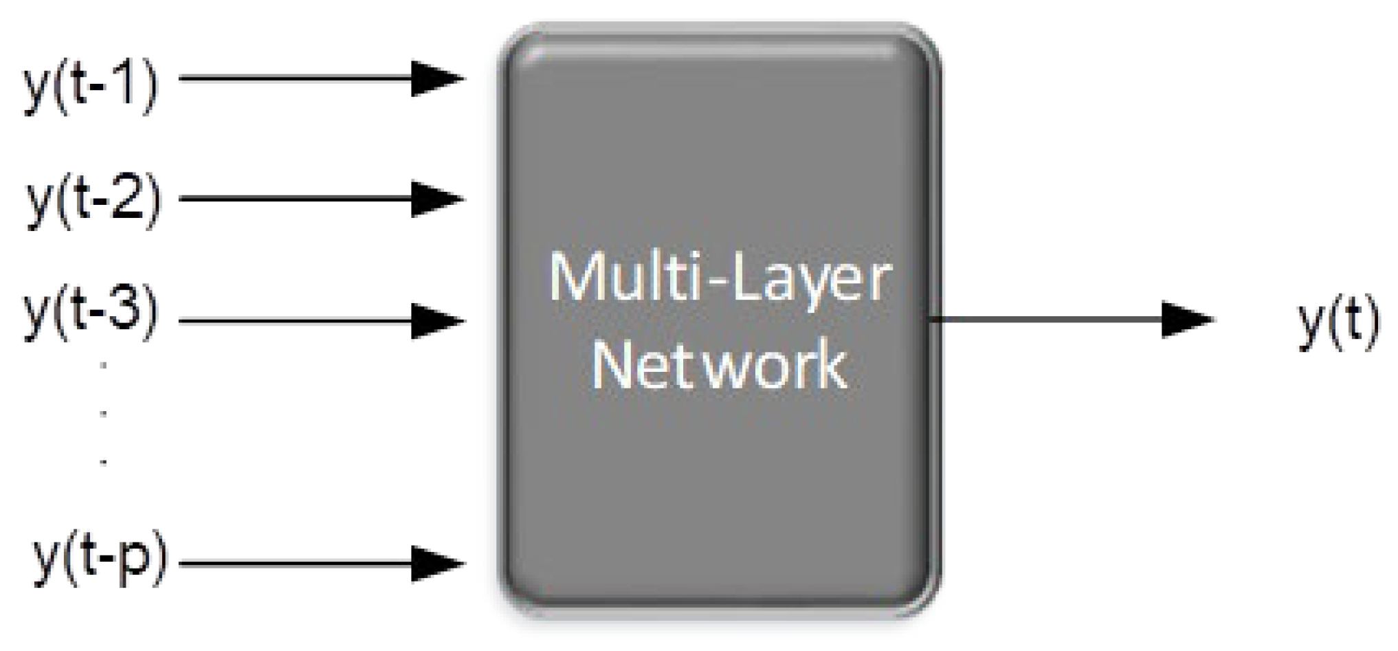
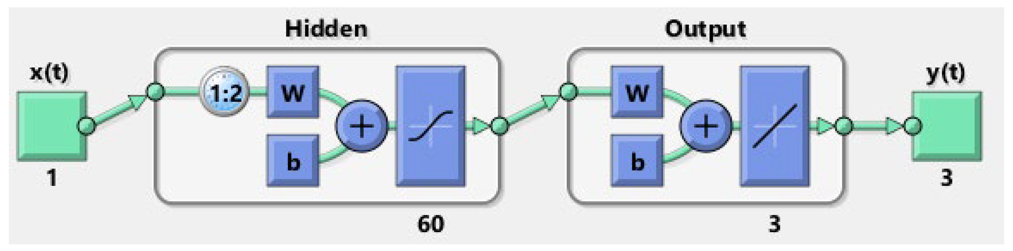
  • An innovative solution scheme based on a two-layer arrangement of LM-SNNs is proposed for the solution of MHD-HFRHT flow model in the form of non-linear ODEs.
  • The MHD-HFRHT flow problem is numerically solved by using “NDSolve” methodology in the Mathematica software. Reference solution in the form of data sets is placed for LM-SNNs for training, validation and the testing of these data sets.
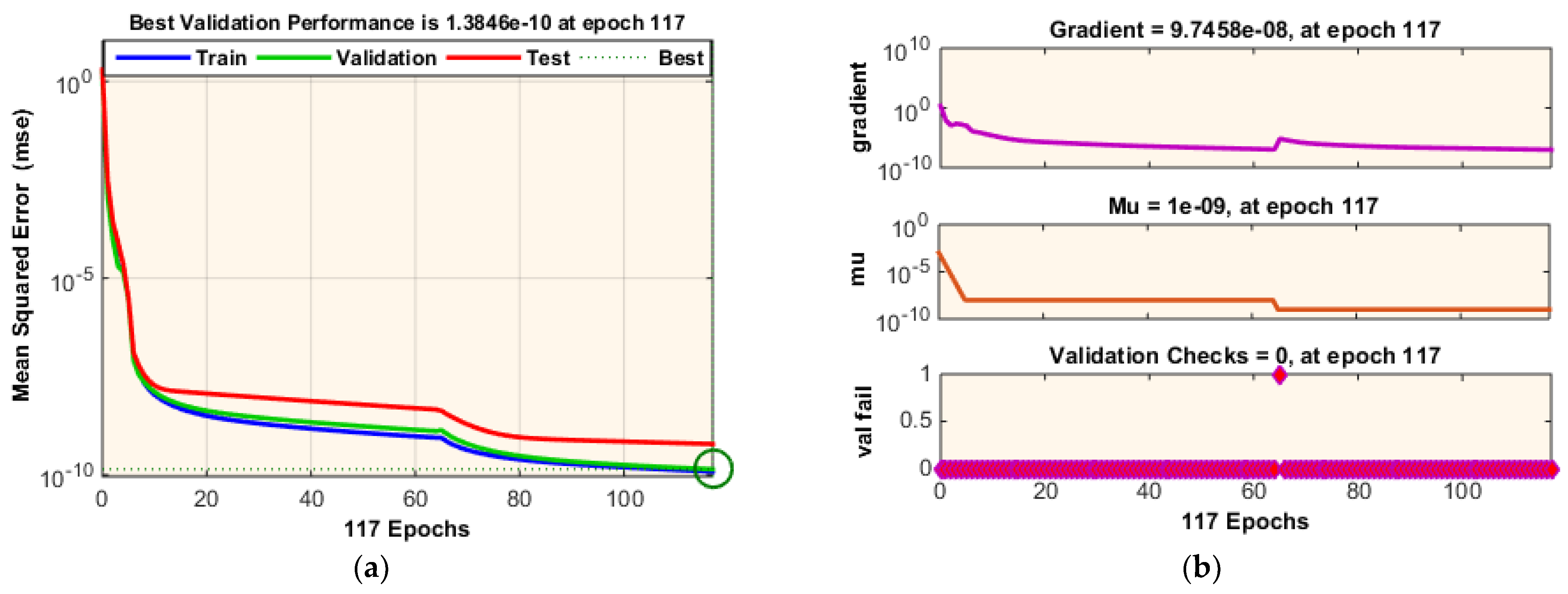
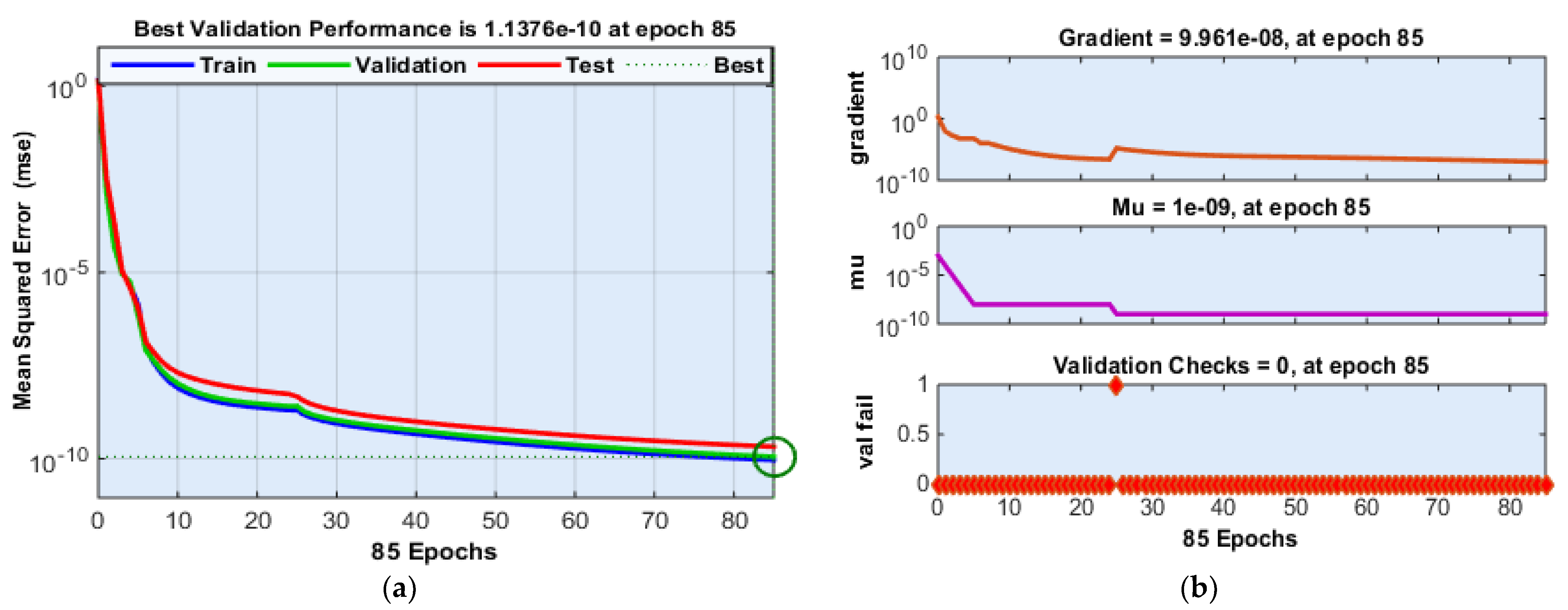
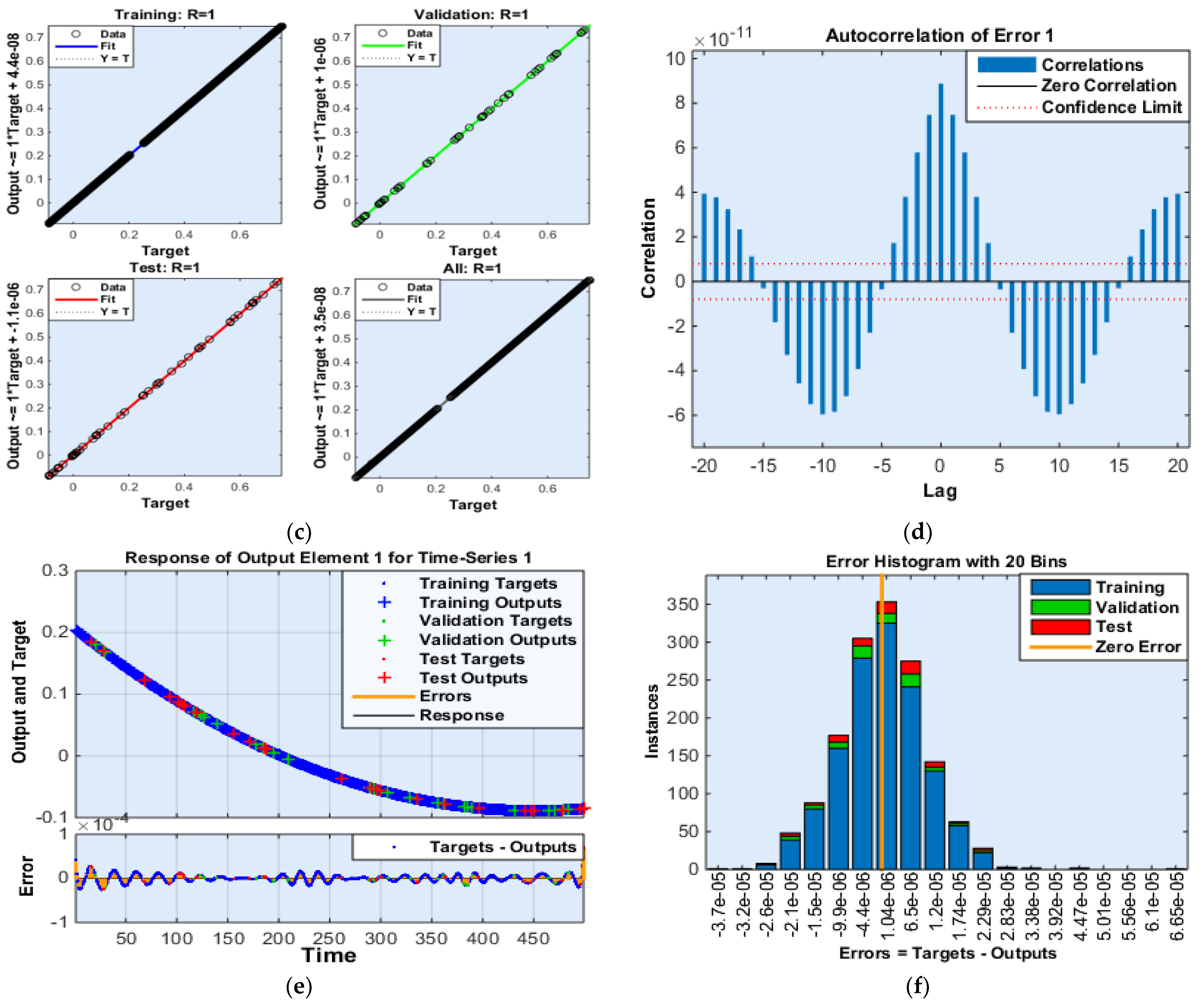
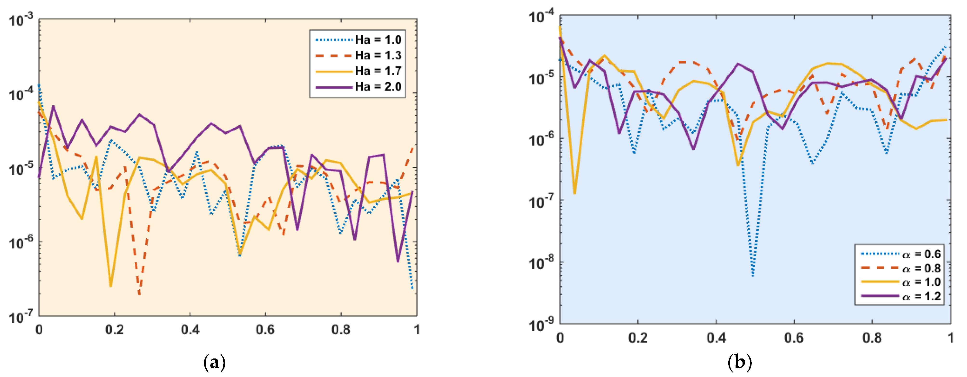
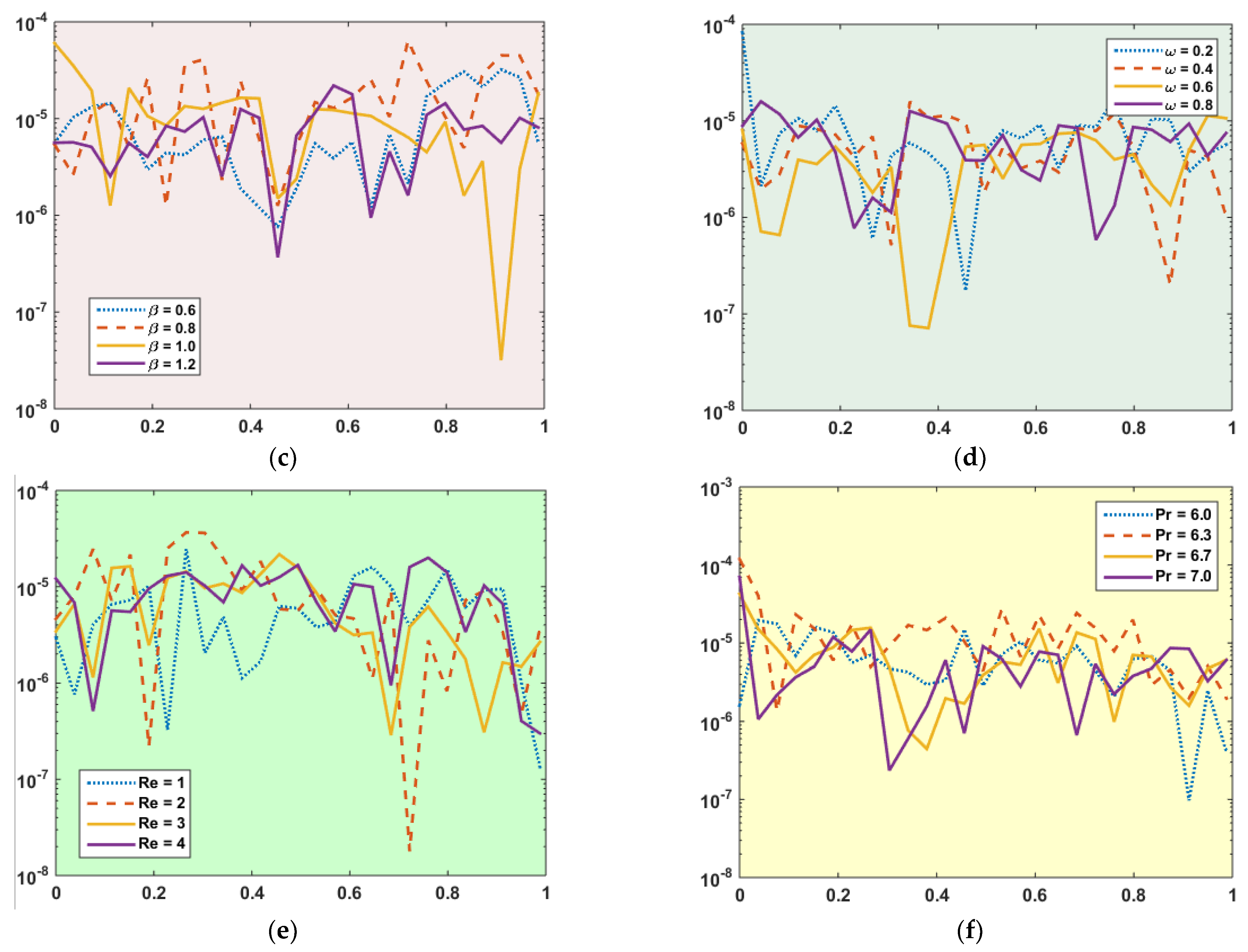
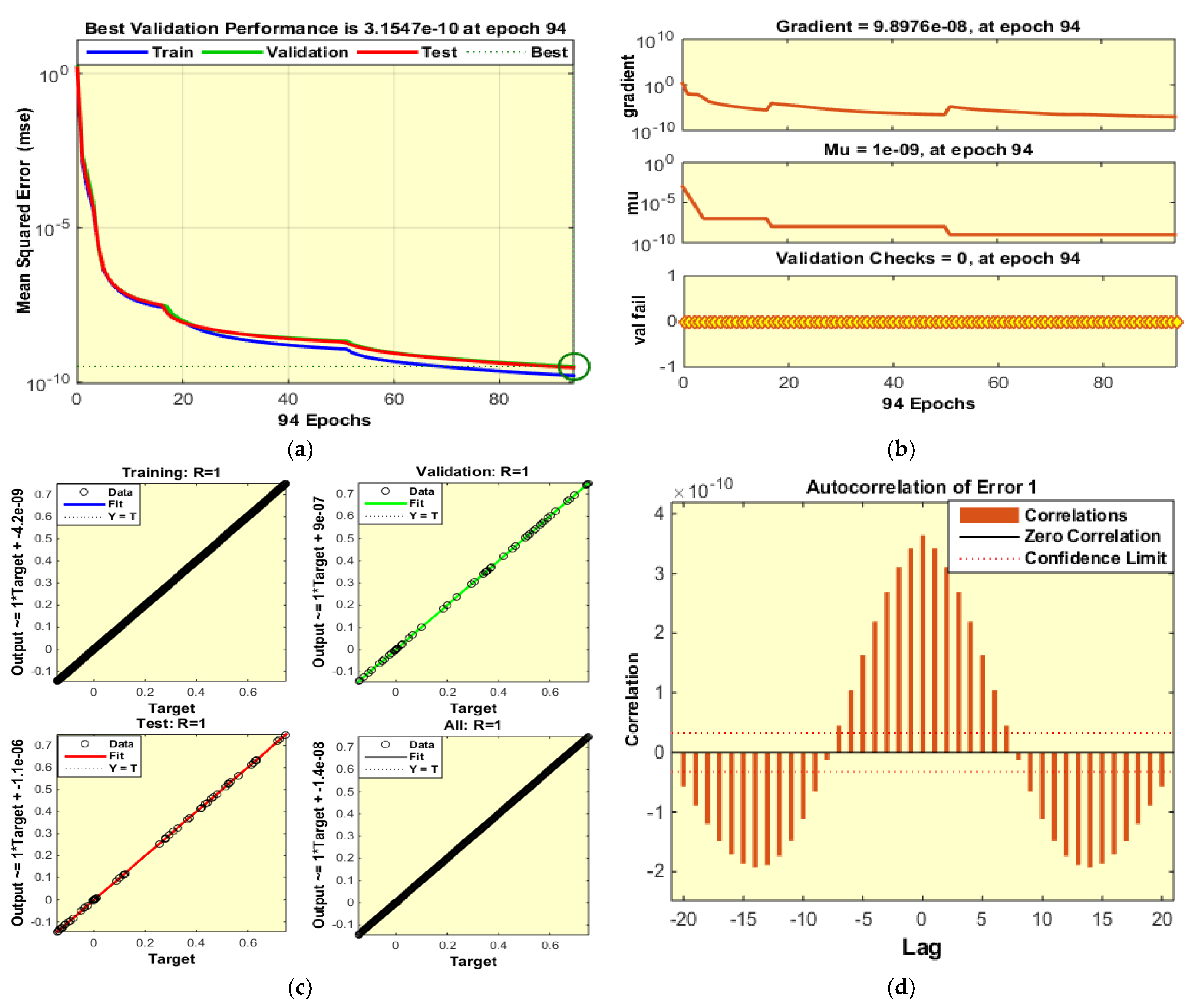
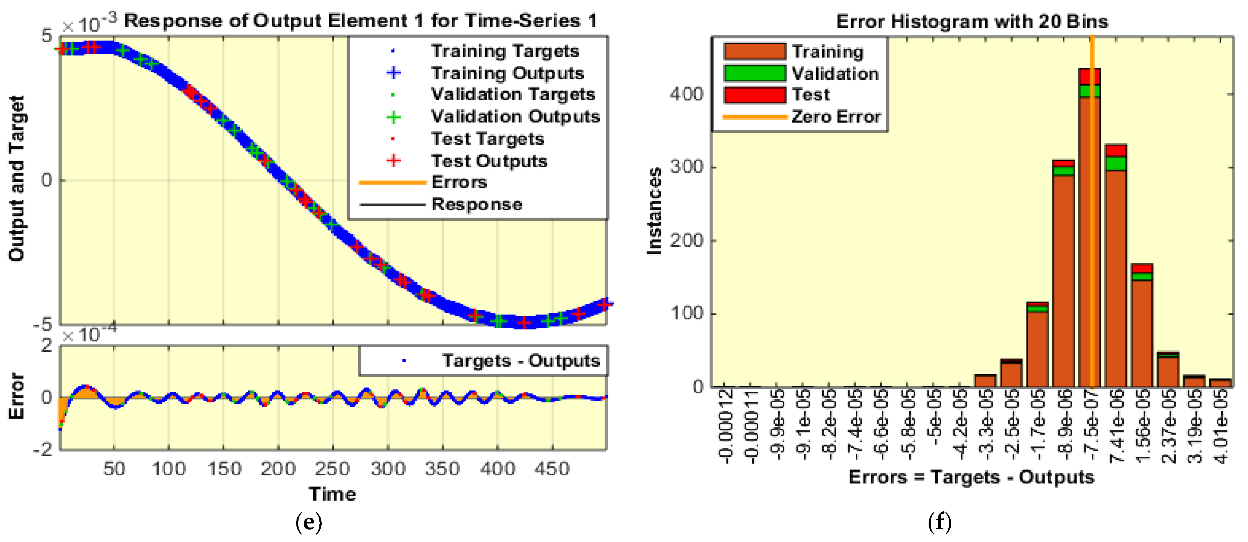
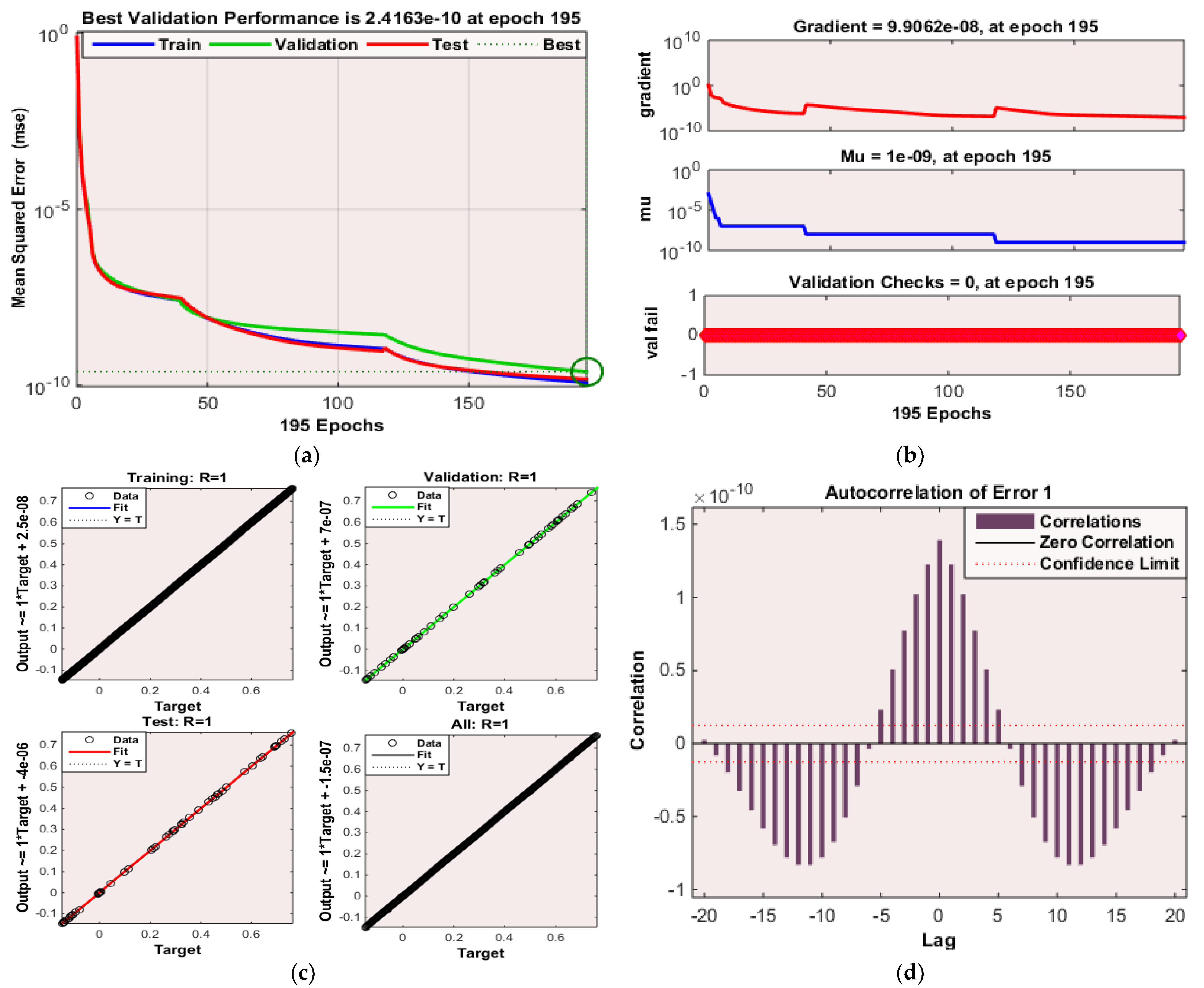
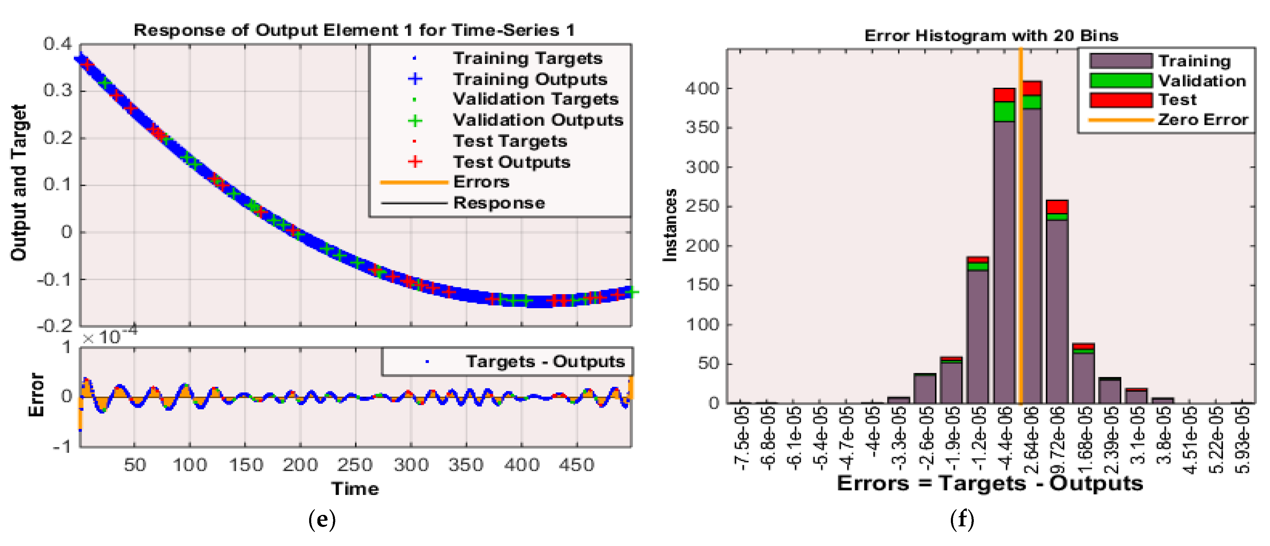
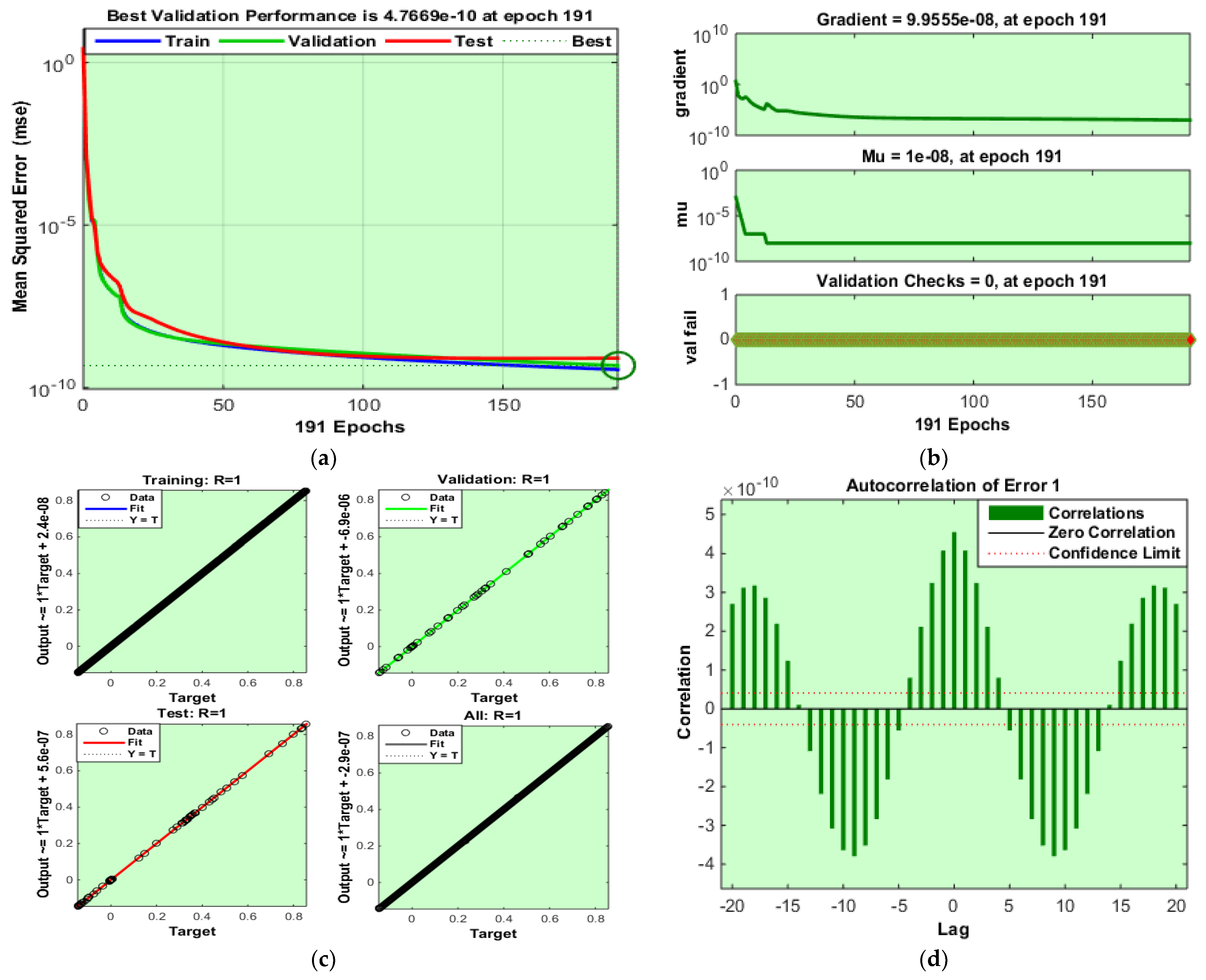
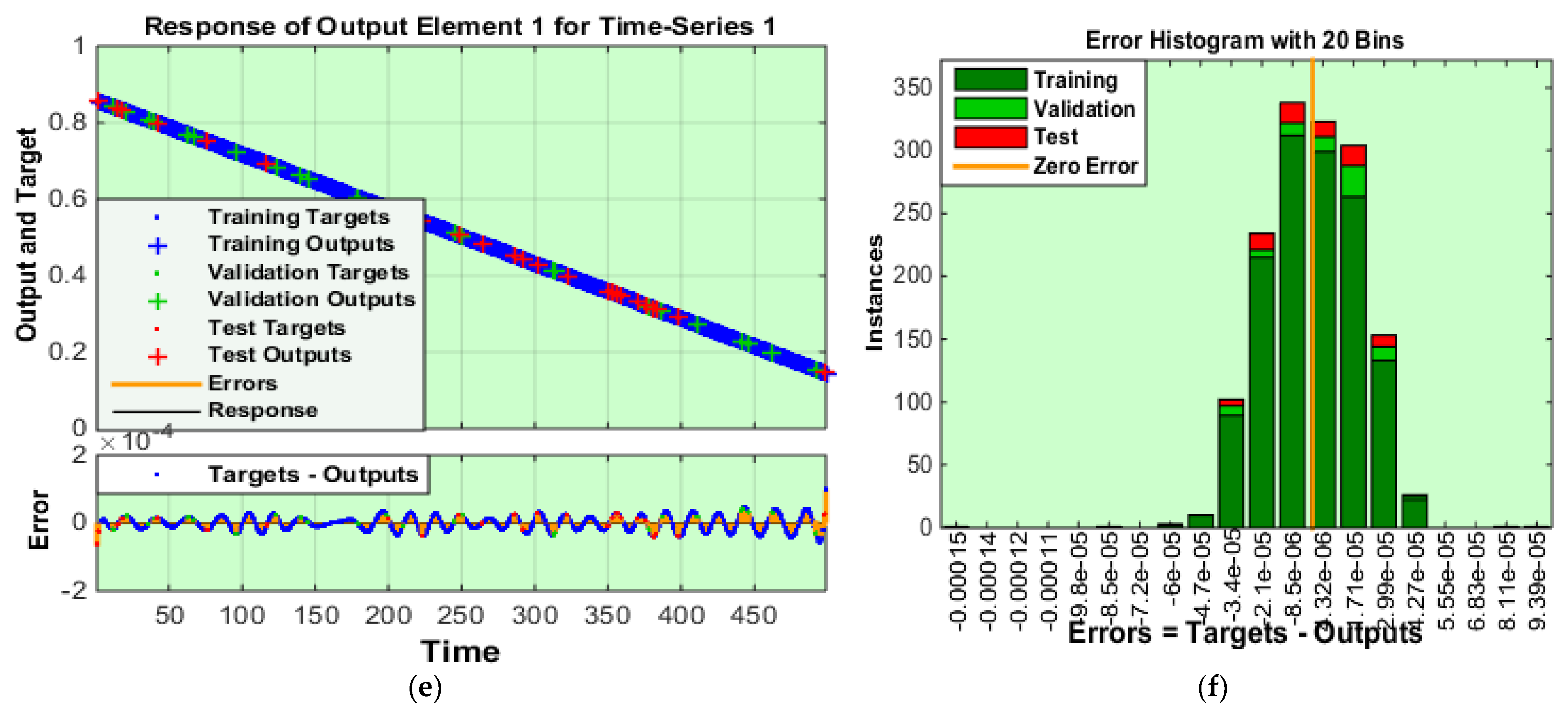
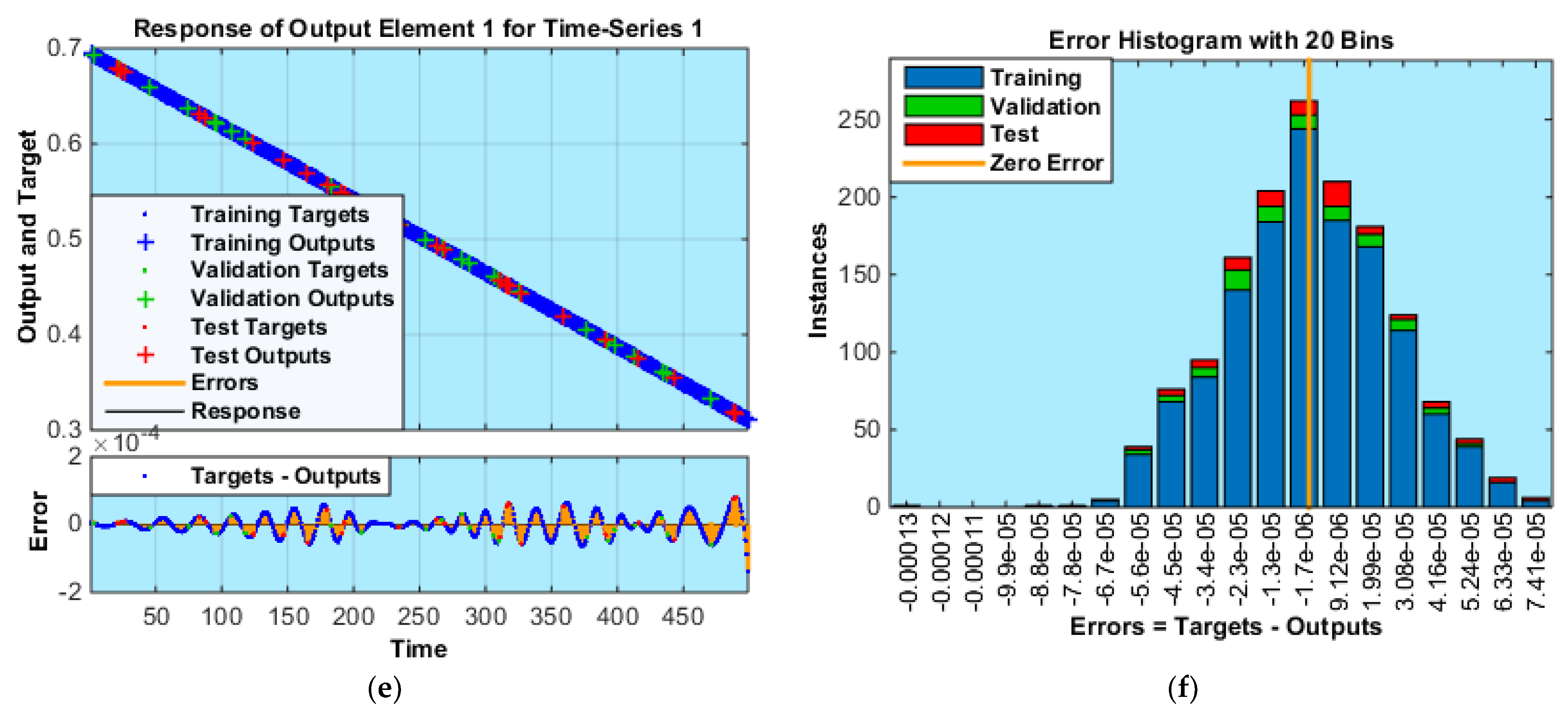
  • Comparison of reference solution with proposed LM-SNNs based solution is authenticated with numerical and graphical results of MSE, regression plots, error-correlation and error histogram which confirm the stability, accuracy, and convergence of solution methodology.
The remainder of the paper is organised as follows: Section 2 provides the mathematical modeling of the flow problem, Section 3 provides the solution methodology, Section 4 comprises the results and discussion and Section 5 provides the conclusion.

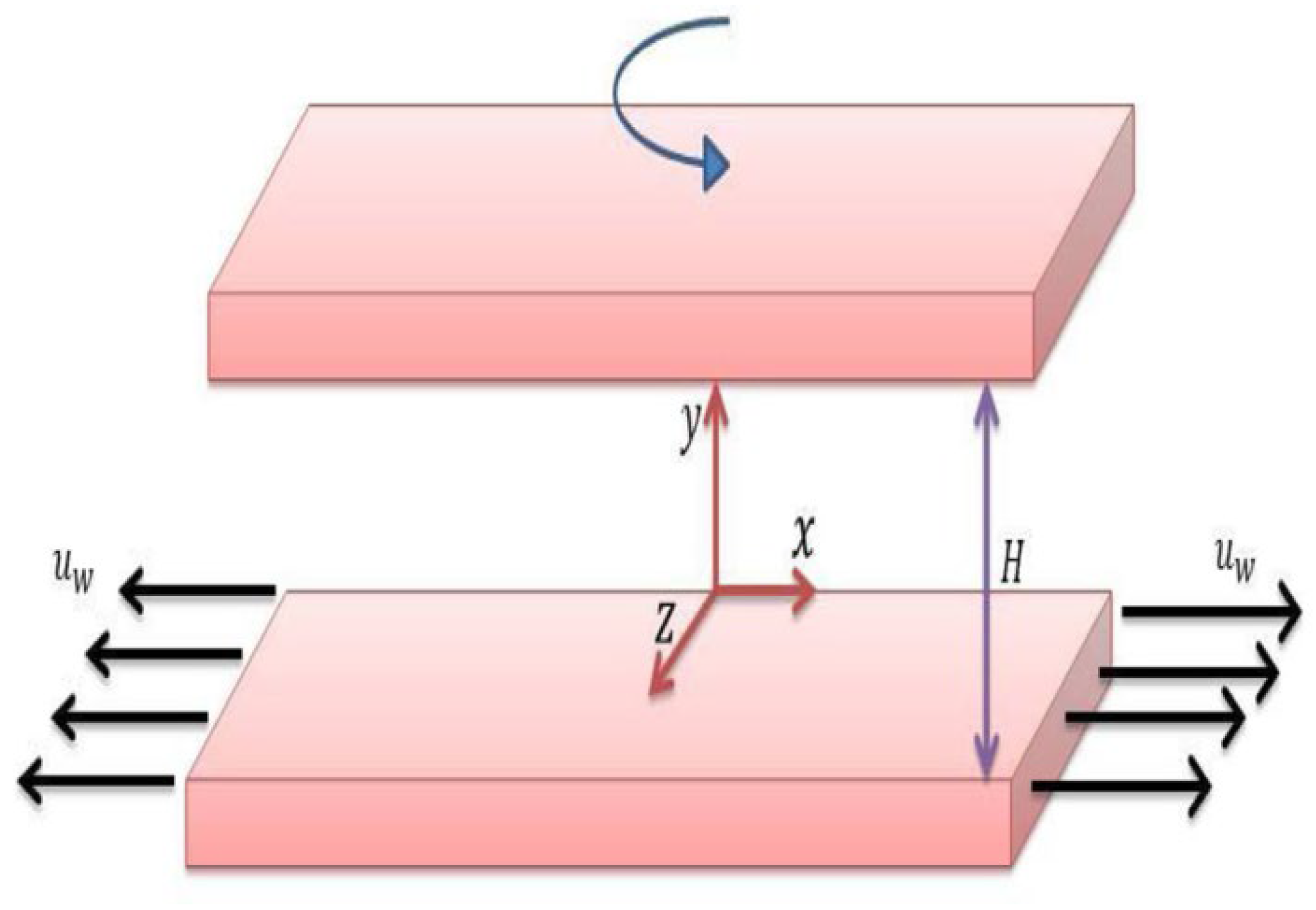
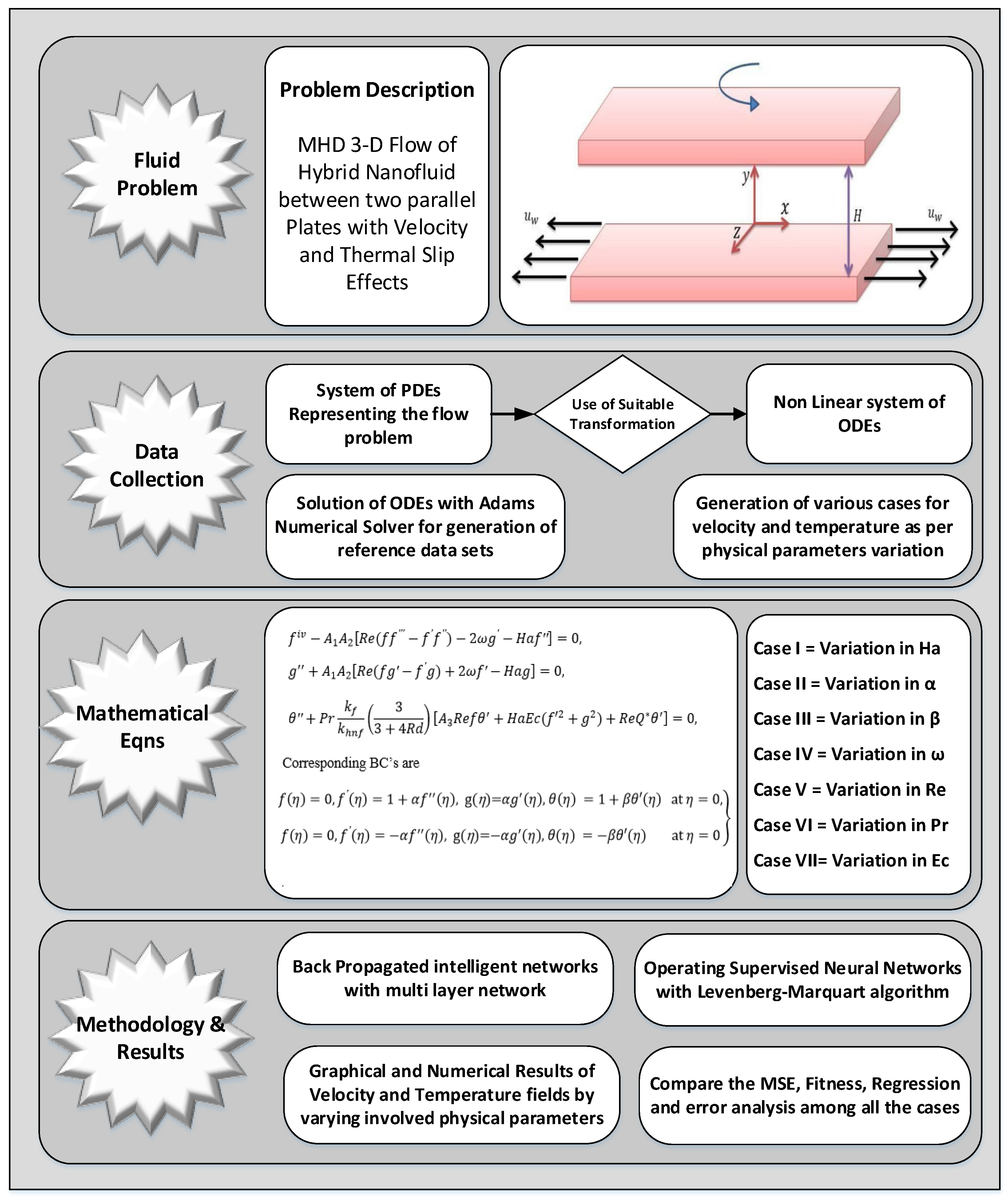
2. Mathematical Formulation of the Problem

Consider the flow of an incompressible and viscous hybrid nanofluid between two parallel plates with stretchable lower plates and velocity and thermal slip effects at both plates. The complete setup rotates around the y-axis with a uniform angular frequency Ω. During the investigation process, the size of all nanoparticles are assumed to be uniform. The nanofluid also considered to be electrically conductive and the induced magnetic field is neglected due to the very small value of the Reynolds number. B0 is the uniform magnetic field acting along the direction parallel to the y-axis (Figure 1). The temperature of the system is influenced by Joule heating and heat generation/absorption effects.
Therefore, keeping in view the above considerations, mathematical expressions representing flow model are [55,56]:
u x + v y = 0 ,
u u x + v u y 2 Ω w = ν h n f [ p x + 2 u x 2 + 2 u y 2 ] σ h n f ρ h n f B 0 2 u ,
u v x + v v y = ν h n f [ p y + 2 v x 2 + 2 v y 2 ] ,
u w x + v w y + 2 Ω u = ν h n f [ 2 w x 2 + 2 w y 2 ] σ h n f ρ h n f B 0 2 w ,
u T x + v T y = ( α h n f + 16 σ * T 0 3 3 k * ( ρ c p ) h n f ) [ 2 T x 2 + 2 T y 2 ] + Q ( ρ c p ) h n f ( T T H ) + σ h n f B 0 2 ( ρ c p ) h n f [ u 2 + w 2 ] .
Subject to the boundary conditions:
When   y = 0   Then     u = a x + L 0 ( u y ) ,     v = 0 , w = L 0 ( w y ) ,   T = T H + L T ( T y ) , When   y = H   Then = L 0 ( u y ) ,   v = 0 ,     w = L 0 ( w y ) ,     T = T 0 L T ( T y ) .
In above system of equations u ,   v   a n d   w are velocity components in the direction parallel to the x, y and z axis respectively. L0 and LT denote the slip coefficients of velocity and temperature respectively, and Ω represents angular frequency, Q is heat coefficient and TH is temperature of fluid at height H. Radiation term in Equation (5) is calculated using the following relationship:
q r = ( 4 σ * 3 k * ) T 4 y
After expending T4 about T0 in above expression by using Taylor’s series, we get
T 4 = 3 T 0 4 + 4 T 0 3 T
The set of transformations mentioned below are employed to transform the system of ODEs into non-linear set of PDEs.
u = a x f ( η ) ,     v = a h g ( η ) ,     w = a x g ( η ) ,                                                     η = y h ,     θ ( η ) = T T H T H T 0 . }
Various Thermo-physical properties can be mathematically expressed as [57]:
μ h n f = μ f [ ( 1 ϕ 1 ) ( 1 ϕ 2 ) ] 2.5 ,     ρ h n f = ρ f [ ( ρ s 1 ρ f ) ϕ 1 + ( 1 + ϕ 1 ) ] ( 1 ϕ 2 ) + ϕ 2 ρ s 2 ,
[ ρ c p ] h n f = [ ρ c p ] f [ ( 1 ϕ 1 ) + ( ρ c p ) s 1 ( ρ c p ) f ϕ 1 ] ( 1 ϕ 2 ) + ϕ 2 ( ρ c p ) s 2 ,     α h n f = k h n f ( ρ c p ) h n f ,            
k h n f k b f = k s 2 + 2 k b f ( s 1 ) ϕ 2 ( k b f k s 2 ) ( s 1 ) ( k b f k s 2 ) ϕ 2 + k b f ( s 1 ) + k s 2 ,       k b f k f = k s 1 + k f ( s 1 ) ϕ 1 ( k f k s 1 ) ( s 1 ) k f ( s 1 ) + ϕ 1 ( k f k s 1 ) + k s 1 ,
σ h n f σ b f = σ s 2 + 2 σ b f ( s 1 ) ϕ 2 ( σ b f σ s 2 ) ( s 1 ) ( σ b f σ s 2 ) ϕ 2 + σ b f ( s 1 ) + σ s 2 ,       σ b f σ f = σ s 1 + σ f ( s 1 ) ϕ 1 ( σ f σ s 1 ) ( s 1 ) σ f ( s 1 ) + ϕ 1 ( σ f σ s 1 ) + σ s 1
The hybrid nanofluid is made up of two types of nanoparticles. ϕ 1 and ϕ 2 represent the solid-volume fraction of nanoparticles Cu and Al2O3 respectively, whereas ϕ h n f is the net solid volume concentration of the hybrid nanoparticles which can be calculated as   ϕ 1 + ϕ 2 . Density of base fluid, density of Cu nanoparticle and density of Al2O3 are represented by ρ f ,     ρ s 1 ,   ρ s 2 ,   respectively. The specific heat and thermal conductivity of Cu nanoparticle, Al2O3 nanoparticle, base fluid and hybrid nanofluid are denoted by k s 1 ,   k s 2 ,   k f   ,   k h n f   ,   ( c p ) s 1 ,   ( c p ) s 2 , ( c p ) f , and   ( c p ) h n f respectively. Table 1 presents the numerical values for various thermophysical properties against base fluid and nanoparticles whereas Figure 2 shows the various shapes and values shape factor of nanoparticles.
Coefficients of skin friction and heat transfer can be expressed mathematically as [11]:
C f = μ h n f ρ f v 0 2 ( u y ) y = 0 ,         C g = μ h n f ρ f v 0 2 ( v y ) y = 0 , N u = h k f ( T f T ) ( k h n f + 16 σ * T H 3 3 k * ) ( T y ) y = 0 ,
Equations (2)–(5) are reduced as
f i v A 1 A 2 [ R e ( f f f f ) 2 ω g H a f ] = 0 ,
g + A 1 A 2 [ R e ( f g f g ) + 2 ω f H a g ] = 0 ,
θ + P r k f k h n f ( 3 3 + 4 R d ) [ A 3 R e f θ + H a E c ( f 2 + g 2 ) + R e Q * θ ] = 0 ,
Here,
A 1 = [ ( 1 ϕ 1 ) ( 1 ϕ 2 ) ] 5 2 ,   A 2 = [ 1 ϕ 2 ] [ ( 1 ϕ 1 ) + ( ρ s 1 ρ f ) ϕ 1 ] + ( ρ s 2 ρ f )   ϕ 2 , A 3 = [ 1 ϕ 2 ] [ ( 1 ϕ 1 ) + ( ( ρ c p ) s 1 ( ρ c p ) f ) ϕ 1 ] + ( ( ρ c p ) s 2 ( ρ c p ) f ) ϕ 2 . }
Corresponding BC’s are
f ( η ) = 0 ,   f ( η ) = 1 + α f ( η ) ,   g ( η ) = α g ( η ) ,   θ ( η ) = 1 + β θ ( η )   at   η = 0 , f ( η ) = 0 ,   f ( η ) = α f ( η ) ,   g ( η ) = α g ( η ) ,   θ ( η ) = β θ ( η )   at   η = 0 }
Non-dimensionalized parameters involved in above equations are:
        α = λ 1 h ,     β = λ 2 h ,     E c = a 2 x 2 ( c p ) f ( T H T 0 ) ,   Ha = σ f B 0 2 a ρ f ,     ω = Ω h 2 ρ f μ f ,     P r = υ f ( ρ c p ) f k f ,   R d = 4 σ * T H 3 k * k f ,   R e = a h 2 ρ f μ f ,       Q * = Q 0 a ( ρ c p ) f .
Here H a represent the Hartman number or Magnetic parameter, Re is the Reynolds number, Ec is the Eckert number, ω is the rotation parameter, Rd is the radiation parameter, Q * is heat generation/absorption coefficient, Pr is the Prandtl number, α is the velocity slip parameter and β is the thermal slip parameter.
Coefficients of skin friction and Nusselt number in non-dimensionalized form are:
C f R e x 1 2 = 1 ( 1 ϕ 1 ) 5 2 ( 1 ϕ 2 ) 5 2 f ( 0 ) , C g R e y 1 2 = 1 ( 1 ϕ 1 ) 5 2 ( 1 ϕ 2 ) 5 2 g ( 0 ) N u Re x 1 2 = ( k h n f k f + 4 R d 3 ) θ ( 0 ) .

3. Solution Methodology

An optimization-based mathematical process generates nonlinear mapping between the input and output layers that intends to convert the human brain into the information acquisition setup, which is known as “Supervised Neural Networks (SNNs)” [60,61,62]. Complete systematic process of the SNNs has been portrayed in Figure 3. The artificial neurons, as a basic component of this network, have the task to obtain the information in terms of input variables and transfer this to the output layers. A nonlinear autoregressive (NAR) network, based on sigmoid function [63], is an effective approach based on SNNs for the prediction and estimation of unknown values for a time series by using the re-feeding mechanism for a defined data set, in which the estimated value may again be used as an input for further prediction of new values. Figure 4 expresses an NAR-based neural network model [64] that contains three different layers, consisting of the input, hidden and output layers with a couple of delay steps, which are used for the estimation of a nonlinear time series, which can be written as [65]:
y ( t ) = h ( y ( t 1 ) ,   y ( t 2 ) ,   y ( t 3 ) , , y ( t d ) ) + ε ( t )
The above expression describes how an NAR based neural network is used to predict or estimate an unknown value at any time “t” based on its previous values with “d” as the time delay parameter. The function h ( * ) in Equation (16) is estimated by the proper training of the network through a given input and adjusting the number of neurons. Whereas ε ( t ) represent the cumulative error of the whole series   y ( t ) .
Hidden layers and the number of neurons are adjusted by keeping in mind the complexity of the model and the desired accuracy of results. A greater number of neurons generates more accurate results but, at the same time, enhances the complexity of the system. On the other side, with less neurons, the computational capabilities of the neural network might be compromised. The most commonly used neural network is based on the backward feeding Levenberg-Marquardt method [66,67]. The basic structure of such a network, with the input and output hidden layers is shown in Figure 5.
The mean square error (MSE) is a valuable tool to illustrate the validity, reliability and accuracy of the computations. Mathematically, the MSE can be expressed as
M S E = i = 1 n ( y i ¯ y i ) 2 n
Here, y i represents the value of ith reference data point, y i ¯ is the value of the ith point obtained with the operation of neural network and the total number of data set points are represented by   n .

4. Results and Discussion

A set of transmuted ODEs (Equations (9)–(11)), expressing the flow model of the MHD-HFRHT problem, is solved in two phases. In the first phase, the said problem is solved by utilizing the “ND Solve” solution methodology in Mathematica software. The solution of the MHD-HFRHT problem, containing the numerical values of   f ( η ) , g ( η )   and θ ( η )   of six scenarios, has four cases according to the variation of parameters as mentioned in Table 2 for each scenario. A total of 500 data set points are formulated for each of the variables f ( η ) ,   g ( η )   a n d   θ ( η ) between a defined domain from 0 to 1 by maintaining the value of step size of 0.005.
In the second phase, these data sets are brought to MATLAB for the implementation of the proposed LM-SNNs. Out of all the imported data set points, 90% are chosen for training purpose in the network, whereas the remaining 5% of data points are subjected for the validation and testing processes of the network. An appropriate number of neurons are selected according to the complexity of the problem and required accuracy of the results. All computational results comprised of MSE, gradients, Mu and error plots showing the validity and performance of proposed LM-SNNs are presented graphically in Figure 6, Figure 7, Figure 8 and Figure 9 and numerically in Table 3.
Figure 6a demonstrates the performance of the network by displaying the Mean square error (MSE) for training, validation and testing for scenario-1 (Variation of Hartman number “Ha”). Mean square error (MSE) of any solution technique estimates the average of the square of errors (difference between target and predicted values) divided by the total number of data points. Smaller values of MSE for any computation technique depicts better accuracy, good performance and the stability of the solution. Figure 6b presents the plots of gradient, Mu and validation checks for each case in scenario-1 (Variation of Hartman number “Ha”). The gradient is some kind of vector with a specific magnitude and direction that is computed during the training of that network. The gradient vector is utilized to update the proposed network in an accurate direction with an exact value. Mu is a parameter that is used to control the applied algorithm in the training of the network. The convergence of the solution is directly dependent on the value of Mu. Figure 6c displays the regression plots for training, validation and testing of the network for scenario-1 (Variation of Hartman number “Ha”). A regression is the statistical measure used to verify the accuracy of the trained model by checking the closeness of predicted data points with the regression line. The value of R very much close to 1 shows that the proposed model prediction is very close to the actual values. If the value of R is 0, the proposed model completely fails to estimate the actual/correct values. A regression value of equal to 1 confirms a close relationship between the predicted and targeted values. Figure 6d exhibits the plot of auto-correlation for scenario-1 (Variation of Hartman number “Ha”). It can be seen that the maximum value lies above the confidence limit set by the network. Figure 6e shows the time series response for scenario-1, through the response of training, validation and testing against their respective targeted values, whereas Figure 6f exhibits the error histogram for the same scenario. The error histogram represents the distribution of errors from the zero line. Each bar of the plot represents the number of values of datasets, which lies in a specific bin. The maximum number of values lies close to the zero-line error, which confirms the accuracy and stability of the method. Figure 7a–f demonstrates performance plots, Grad plots, regression plots, error auto-correlation plots, time series response and error histograms for the scenario 2 of the computations (Variation of   α ). Additionally, the same set of plots for scenarios 3~6 are presented in the Appendix A in Figure A1, Figure A2, Figure A3 and Figure A4, respectively.
A comparison of the proposed LM-SNNs based solution with the referenced numerical solution for f ( η ) against variation of Ha and α are presented in Figure 8a,b. In the figures, the impact of the Hartmann number on velocity is given, demonstrating the decrement of velocity significantly due to an increase in the Hartmann number, while a very minimal impact of the velocity slip parameter on the velocity profile is observed. This occurs as the Hartmann number measures the relative significance of drag force that derives from the magnetic induction of the velocity of the fluid flow system. Similarly, a comparison of the proposed LM-SNNs based solution with reference numerical solution for g ( η ) against variation of ω and Re are presented in Figure 8c,d. In these figures, it can be seen that the vertical component of velocity is significantly enhanced due to the rotation parameter, while the radiation parameter does not influence the vertical components considerably. An identical comparison of the proposed solution with the referenced numerical solution for θ ( η ) against ω and β is presented in Figure 8e,f. In these subfigures thermal slip reduced the temperature profile, but the rotation parameter does not affect the temperature profile significantly. The absolute error (AE) represents the uncertainty in the measurement and calculated as the difference between the actual and calculated value of a quantity. The absolute error is used to express the reliability of computation and inconsistency in measurement. Figure 9a–f presents a comparison of the absolute error (AE) for various scenarios.

5. Conclusions

In the present work, the MHD-HRHT model was solved and investigated by employing the computational strength of LM-SNNs. A conventional data set for velocity and temperature variable has been generated, out of which 90%, 5% and 5% of the points are used for training, validation and for testing the network, respectively. This reference solution is then compared with the result of the proposed LM-SNNs solution. An MSE of up to 1e-11 and excellent distribution of error validates the convergence, accuracy and stability of the proposed LM-SNN Model. A variety of graphical and numerical outcomes, which consist of MSE, error histograms, regression plots and time series responses are presented. Some of the major findings of the research are as follows:
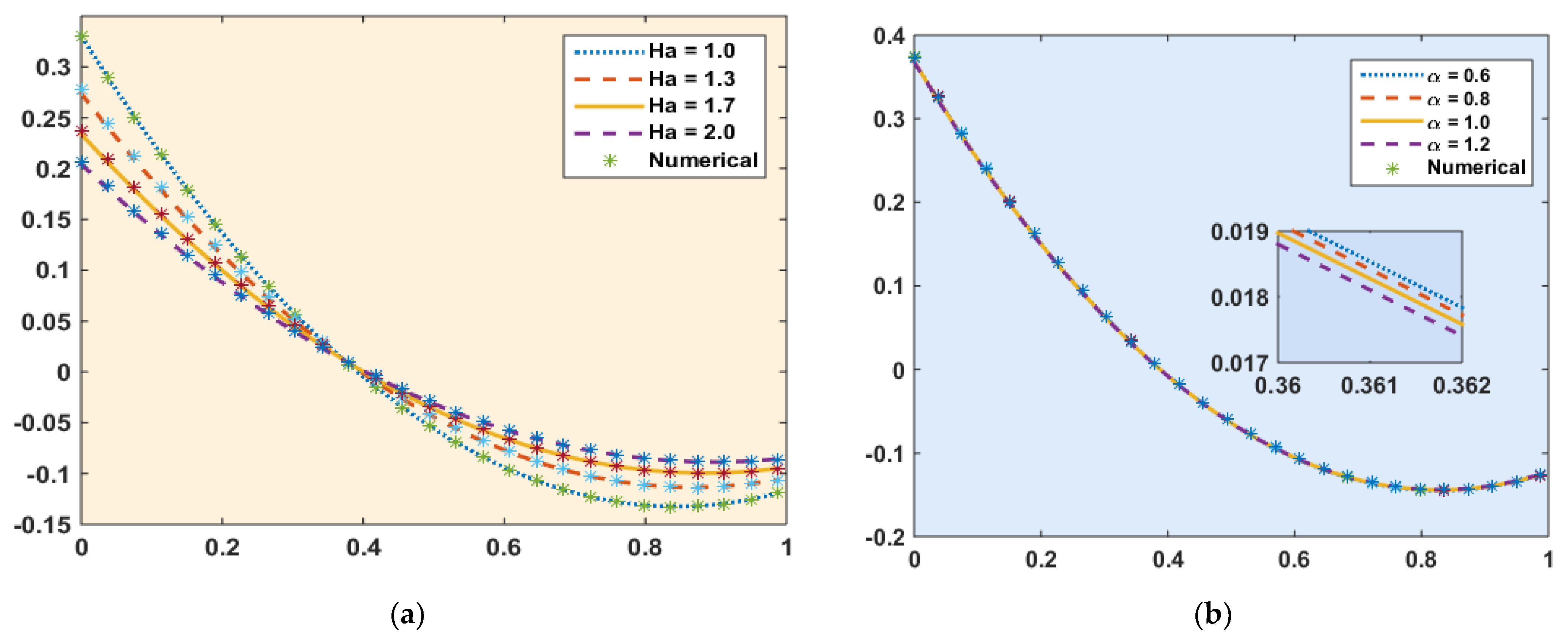
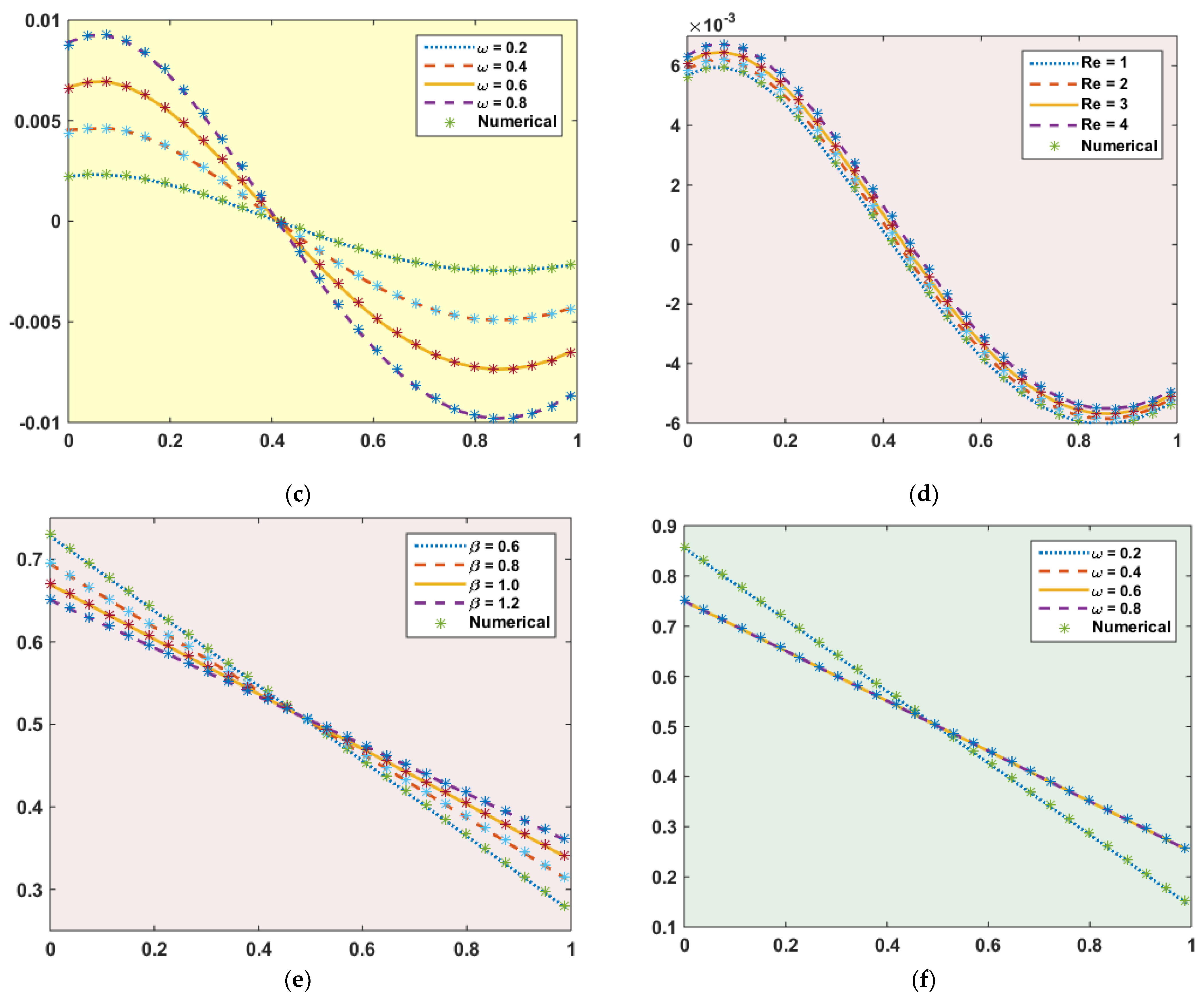
  • By increasing the Hartmann number there more resistance to flow which results in the reduction of velocity. This happens as the Hartmann number measures the relative implication of drag force derived from the magnetic induction of the velocity of the fluid flow system.
  • Velocity of the fluid enhances with higher values of the Reynolds number due to the strength of the inertial force. Moreover, the rotation parameter also accelerates the velocity of the fluid-flow system.
  • Temperature profile declines with an increase in the Hartmann number and thermal slip parameter.
  • With the larger values of Prandtl due to which momentum diffusivity dominates over thermal diffusivity, are a result of the decrease in the temperature profile.
  • Temperature profile decreases for high values of Eckert numbers, which is due to dominating bulk transport of the fluid flow.
In future studies, modern solution methodologies, based on artificial intelligence and machine learning, will be established to investigate the fluid flow problem [68,69,70,71,72,73,74,75,76] more efficiently.

Author Contributions

Conceptualization, M.S., M.A.Z.R. and M.T.S.; methodology, M.S. and K.S.N.; software, M.S., M.A.Z.R., M.T.S., K.S.N. and W.J.; validation, M.A.Z.R., M.T.S. and W.J.; formal analysis, K.S.N., B.F.F. and I.S.Y.; investigation, M.S., M.A.Z.R., M.T.S. and K.S.N.; resources, M.S., K.S.N., B.F.F. and I.S.Y.; writing—original draft preparation, M.S., M.A.Z.R., M.T.S., K.S.N. and W.J.; writing—review and editing, M.S., K.S.N., B.F.F. and I.S.Y.; visualization, M.A.Z.R. and M.T.S.; funding acquisition, K.S.N., B.F.F. and I.S.Y. All authors have read and agreed to the published version of the manuscript.

Funding

This work was received funding from King Khalid University, Ministry of Education and Taif University, all in Saudi Arabia.

Institutional Review Board Statement

Not applicable.

Informed Consent Statement

Not applicable.

Data Availability Statement

Not applicable.

Acknowledgments

The authors express their appreciation to the Deanship of Scientific Research at King Khalid University for funding this work through the research groups program under grant number R.G.P.2/110/41. Also, the authors extend their appreciation to the Deputyship for Research & Innovation, Ministry of Education, in Saudi Arabia for funding this research work through the project number: (IFP-KKU-2020/10). Bassem F. Felemban acknowledges Taif University Researchers Supporting Project number (TURSP-2020/260), Taif University, Taif, Saudi Arabia. All authors are thankful to the referees for their critical comments which improved the paper.

Conflicts of Interest

The authors declare no conflict of interest.

Nomenclature

Symbols
u, v, wVelocity components
kThermal Conductivity
TTemperature
L0Velocity slip coefficient
ReReynolds Number
f, gTransformed components of velocity
CPSpecific Heat
θTransformed temperature
LTThermal slip coefficient
NuPrandtl Number
Subscripts
nfNanofluid
hnfHybrid nanofluid
Greek Letters
ρDensity
μViscosity
ηTransformed coordinate
σElectrical conductivity
ϕ Nano particle Volume fraction
αTransformed velocity slip parameter
βTransformed thermal slip parameter
ωRotation parameter
Abbreviations
MHDMagnetohydrodynamics
MSEMean square error
PDEsPartial differential equations
CNTsCarbon nanotubes
ODEsOrdinary differential equations
AEAbsolute error
HFRHTHybrid nanofluid flow due to rotating disk with heat absorption and thermal slip effects

Appendix A

The outcomes of proposed computing solver LM-SNNs for scenario 3 to 8 of MHD-HFRHT are provided in Figure A1, Figure A2, Figure A3 and Figure A4.
Figure A1. Comparison of various plots against variation of ω (Scenario 4-Case 2). (a): Plot for Mean Square Error; (b): Plots for Mu, Grad and Validation; (c): Regression Plots; (d): Plot for Error Auto Correlation; (e):Time Fitness Plot; (f): Error histogram Plots.
Coatings 11 01554 g0a1aCoatings 11 01554 g0a1b
Figure A2. Comparison of various plots against variation of Re (Scenario 5-Case 2). (a): Plot for Mean Square Error; (b): Plots for Mu, Grad and Validation; (c): Regression Plots; (d): Plot for Error Auto Correlation; (e): Time Fitness Plot; (f): Error Histogram.
Coatings 11 01554 g0a2aCoatings 11 01554 g0a2b
Figure A3. Comparison of various plots against variation of Pr (Scenario 6-Case 1). (a): Plot for Mean Square Error; (b): Plots for Mu, Grad and Validation; (c): Regression Plots; (d): Plot for Error Auto Correlation; (e): Time Fitness Plot; (f): Error Histogram.
Coatings 11 01554 g0a3aCoatings 11 01554 g0a3b
Figure A4. Comparison of various plots against variation of β (Scenario 3-Case 2). (a): Plot for Mean Square Error; (b): Plots for Mu, Grad and Validation; (c): Regression Plots; (d): Plot for Error Auto Correlation; (e): Time Fitness Plot; (f): Error Histogram.
Coatings 11 01554 g0a4aCoatings 11 01554 g0a4b

References

  1. Chi, S.U.; Eastman, J.A. Enhancing Thermal Conductivity of Fluids with Nanoparticles; Argonne National Lab: Lemont, IL, USA, 1995; No. ANL/MSD/CP-84938; CONF-951135-29. [Google Scholar]
  2. Kang, H.U.; Kim, S.H.; Oh, J.M. Estimation of Thermal Conductivity of Nanofluid Using Experimental Effective Particle Volume. Exp. Heat Transf. 2006, 19, 181–191. [Google Scholar] [CrossRef]
  3. Lee, S.; Choi, S.S.; Li, S.A.; Eastman, J.A. Measuring thermal conductivity of fluids containing oxide nanoparticles. J. Heat Transf. 1999, 121, 280–289. [Google Scholar] [CrossRef]
  4. Babar, H.; Ali, H.M. Towards hybrid nanofluids: Preparation, thermophysical properties, applications, and challenges. J. Mol. Liq. 2019, 281, 598–633. [Google Scholar] [CrossRef]
  5. Babu, J.R.; Kumar, K.K.; Rao, S.S. State-of-art review on hybrid nanofluids. Renew. Sustain. Energy Rev. 2017, 77, 551–565. [Google Scholar] [CrossRef]
  6. Gulzar, O.; Qayoum, A.; Gupta, R. Experimental study on stability and rheological behaviour of hybrid Al2O3-TiO2 Therminol-55 nanofluids for concentrating solar collectors. Powder Technol. 2019, 352, 436–444. [Google Scholar] [CrossRef]
  7. Shah, T.R.; Ali, H.M. Applications of hybrid nanofluids in solar energy, practical limitations and challenges: A critical review. Sol. Energy 2019, 183, 173–203. [Google Scholar] [CrossRef]
  8. Yang, L.; Ji, W.; Mao, M.; Huang, J.N. An updated review on the properties, fabrication and application of hybrid-nanofluids along with their environmental effects. J. Clean. Prod. 2020, 257, 120408. [Google Scholar] [CrossRef]
  9. Shoaib, M.; Raja, M.A.Z.; Sabir, M.T.; Islam, S.; Shah, Z.; Kumam, P.; Alrabaiah, H. Numerical investigation for rotating flow of MHD hybrid nanofluid with thermal radiation over a stretching sheet. Sci. Rep. 2020, 10, 1–15. [Google Scholar] [CrossRef]
  10. Rajesh, V.; Chamkha, A.; Kavitha, M. Numerical investigation of Ag-CuO/water hybrid nanofluid flow past a moving oscillating cylinder with heat transfer. Math. Methods Appl. Sci. 2020, 1–16. [Google Scholar] [CrossRef]
  11. Devi, S.S.U.; Devi, S.A. Numerical investigation of three-dimensional hybrid Cu–Al2O3/water nanofluid flow over a stretching sheet with effecting Lorentz force subject to Newtonian heating. Can. J. Phys. 2016, 94, 490–496. [Google Scholar] [CrossRef]
  12. Nagoor, A.H.; Alaidarous, E.S.; Sabir, M.T.; Shoaib, M.; Raja, M.A.Z. Numerical treatment for three-dimensional rotating flow of carbon nanotubes with Darcy–Forchheimer medium by the Lobatto IIIA technique. AIP Adv. 2020, 10, 025016. [Google Scholar] [CrossRef] [Green Version]
  13. Alempour, S.M.; Arani, A.A.A.; Najafizadeh, M.M. Numerical investigation of nanofluid flow characteristics and heat transfer inside a twisted tube with elliptic cross section. J. Therm. Anal. Calorim. 2020, 140, 1237–1257. [Google Scholar] [CrossRef]
  14. Ouyang, C.; Akhtar, R.; Raja, M.A.Z.; Touseef Sabir, M.; Awais, M.; Shoaib, M. Numerical treatment with Lobatto IIIA technique for radiative flow of MHD hybrid nanofluid (Al2O3—Cu/H2O) over a convectively heated stretchable rotating disk with velocity slip effects. AIP Adv. 2020, 10, 055122. [Google Scholar] [CrossRef]
  15. Waini, I.; Ishak, A.; Pop, I. Transpiration effects on hybrid nanofluid flow and heat transfer over a stretching/shrinking sheet with uniform shear flow. Alex. Eng. J. 2020, 59, 91–99. [Google Scholar] [CrossRef]
  16. Afridi, M.I.; Tlili, I.; Goodarzi, M.; Osman, M.; Alam Khan, N. Khan Irreversibility Analysis of Hybrid Nanofluid Flow over a Thin Needle with Effects of Energy Dissipation. Symmetry 2019, 11, 663. [Google Scholar] [CrossRef] [Green Version]
  17. Shafiq, A.; Sindhu, T.N.; Khalique, C.M. Numerical investigation and sensitivity analysis on bioconvective tangent hyperbolic nanofluid flow towards stretching surface by response surface methodology. Alex. Eng. J. 2020, 59, 4533–4548. [Google Scholar] [CrossRef]
  18. Nadeem, S.; Abbas, N.; Malik, M. Inspection of hybrid based nanofluid flow over a curved surface. Comput. Methods Progr. Biomed. 2020, 189, 105193. [Google Scholar] [CrossRef]
  19. Anuar, N.S.; Bachok, N.; Pop, I. Radiative hybrid nanofluid flow past a rotating permeable stretching/shrinking sheet. Int. J. Numer. Methods Heat Fluid Flow 2020, 31, 914–932. [Google Scholar] [CrossRef]
  20. Sreedevi, P.; Reddy, P.S.; Chamkha, A. Heat and mass transfer analysis of unsteady hybrid nanofluid flow over a stretching sheet with thermal radiation. SN Appl. Sci. 2020, 2, 1–15. [Google Scholar] [CrossRef]
  21. Venkateswarlu, B.; Satya Narayana, P.V. Cu-Al2O3/H2O hybrid nanofluid flow past a porous stretching sheet due to temperatue-dependent viscosity and viscous dissipation. Heat Transf. 2020, 50, 432–449. [Google Scholar] [CrossRef]
  22. Ahmed, N.; Khan, U.; Mohyud-Din, S.T. Influence of shape factor on flow of magneto-nanofluid squeezed between parallel disks. Alex. Eng. J. 2018, 57, 1893–1903. [Google Scholar] [CrossRef]
  23. Kandasamy, R.; Adnan, N.A.B.; Mohammad, R. Nanoparticle shape effects on squeezed MHD flow of water based Cu, Al2O3 and SWCNTs over a porous sensor surface. Alex. Eng. J. 2018, 57, 1433–1445. [Google Scholar] [CrossRef]
  24. Shoaib, M.; Raja, M.A.Z.; Sabir, M.T.; Awais, M.; Islam, S.; Shah, Z.; Kumam, P. Numerical analysis of 3-D MHD hybrid nanofluid over a rotational disk in presence of thermal radiation with Joule heating and viscous dissipation effects using Lobatto IIIA technique. Alex. Eng. J. 2021, 60, 3605–3619. [Google Scholar] [CrossRef]
  25. Wang, X.-Q.; Mujumdar, A.S. A review on nanofluids—Part I: Theoretical and numerical investigations. Braz. J. Chem. Eng. 2008, 25, 613–630. [Google Scholar] [CrossRef] [Green Version]
  26. Reiner, M. A Mathematical Theory of Dilatancy. Am. J. Math. 1945, 67, 350. [Google Scholar] [CrossRef]
  27. Rivlin, R.S. The hydrodynamics of non-Newtonian fluids. I. Proc. R Soc. Lond. Ser. A Math. Phys. Sci. 1948, 193, 260–281. [Google Scholar]
  28. Ellahi, R.; Zeeshan, A.; Abbas, T.; Hussain, F. Thermally Charged MHD Bi-Phase Flow Coatings with Non-Newtonian Nanofluid and Hafnium Particles along Slippery Walls. Coatings 2019, 9, 300. [Google Scholar] [CrossRef] [Green Version]
  29. Ellahi, R.; Alamri, S.Z.; Basit, A.; Majeed, A. Effects of MHD and slip on heat transfer boundary layer flow over a moving plate based on specific entropy generation. J. Taibah Univ. Sci. 2018, 12, 476–482. [Google Scholar] [CrossRef] [Green Version]
  30. Alamri, S.Z.; Khan, A.A.; Azeez, M.; Ellahi, R. Effects of mass transfer on MHD second grade fluid towards stretching cylinder: A novel perspective of Cattaneo–Christov heat flux model. Phys. Lett. A 2018, 383, 276–281. [Google Scholar] [CrossRef]
  31. Yousif, M.A.; Ismael, H.F.; Abbas, T.; Ellahi, R. Numerical study of momentum and heat transfer of MHD Carreau nanofluid over an exponentially stretched plate with internal heat source/sink and radiation. Heat Transf. Res. 2019, 50, 649–658. [Google Scholar] [CrossRef]
  32. Pal, D.; Chatterjee, D.; Vajravelu, K. Influence of magneto-thermo radiation on heat transfer of a thin nanofluid film with non-uniform heat source/sink. Propuls. Power Res. 2020, 9, 169–180. [Google Scholar] [CrossRef]
  33. Iqbal, S.A.; Sajid, M.; Mahmood, K.; Naveed, M.; Khan, M.Y. An iterative approach to viscoelastic boundary layer flows with heat source/sink and thermal radiation. Therm. Sci. 2019, 24, 1275–1284. [Google Scholar] [CrossRef] [Green Version]
  34. Ramadevi, B.; Kumar, K.A.; Sugunamma, V.; Sandeep, N. Influence of non-uniform heat source/sink on the three-dimensional magnetohydrodynamic Carreau fluid flow past a stretching surface with modified Fourier’s law. Pramana 2019, 93, 86. [Google Scholar] [CrossRef]
  35. Wang, C.F.; Kafle, B.; Tesema, T.E.; Kookhaee, H.; Habteyes, T.G. Molecular Sensitivity of Near-Field Vibrational Infrared Imaging. J. Phys. Chem. C 2020, 124, 21018–21026. [Google Scholar] [CrossRef]
  36. Mozaffari, S.; Tchoukov, P.; Mozaffari, A.; Atias, J.; Czarnecki, J.; Nazemifard, N. Capillary driven flow in nanochannels–Application to heavy oil rheology studies. Colloids Surf. A Physicochem. Eng. Asp. 2017, 513, 178–187. [Google Scholar] [CrossRef]
  37. Ghasemi, H.; Mozaffari, S.; Mousavi, S.H.; Aghabarari, B.; Abu-Zahra, N. Decolorization of wastewater by heterogeneous Fenton reaction using MnO2-Fe3O4/CuO hybrid catalysts. J. Environ. Chem. Eng. 2021, 9, 105091. [Google Scholar] [CrossRef]
  38. Tesema, T.E.; Kookhaee, H.; Habteyes, T.G. Extracting Electronic Transition Bands of Adsorbates from Molecule–Plasmon Excitation Coupling. J. Phys. Chem. Lett. 2020, 11, 3507–3514. [Google Scholar] [CrossRef]
  39. Khan, I.; Raja, M.A.Z.; Shoaib, M.; Kumam, P.; Alrabaiah, H.; Shah, Z.; Islam, S. Design of Neural Network With Levenberg-Marquardt and Bayesian Regularization Backpropagation for Solving Pantograph Delay Differential Equations. IEEE Access 2020, 8, 137918–137933. [Google Scholar] [CrossRef]
  40. Sabir, Z.; Saoud, S.; Raja, M.A.Z.; Wahab, H.A.; Arbi, A. Heuristic computing technique for numerical solutions of nonlinear fourth order Emden–Fowler equation. Math. Comput. Simul. 2020, 178, 534–548. [Google Scholar] [CrossRef]
  41. Jafarian, A.; Mokhtarpour, M.; Baleanu, D. Artificial neural network approach for a class of fractional ordinary differential equation. Neural Comput. Appl. 2016, 28, 765–773. [Google Scholar] [CrossRef]
  42. Almalki, M.M.; Alaidarous, E.S.; Maturi, D.A.; Raja, M.A.Z.; Shoaib, M. Intelligent computing technique based supervised learning for squeezing flow model. Sci. Rep. 2021, 11, 1–15. [Google Scholar] [CrossRef] [PubMed]
  43. Raja, M.A.Z.; Shoaib, M.; Tabassum, R.; Khan, M.I.; Gowda, R.J.P.; Prasannakumara, B.C.; Malik, M.Y.; Xia, W.-F. Intelligent computing for the dynamics of entropy optimized nanofluidic system under impacts of MHD along thick surface. Int. J. Mod. Phys. B 2021, 35, 2150269. [Google Scholar] [CrossRef]
  44. Ebrahimi, A.; Tamnanloo, J.; Mousavi, S.H.; Miandoab, E.S.; Hosseini, E.; Ghasemi, H.; Mozaffari, S. Discrete-Continuous Genetic Algorithm for Designing a Mixed Refrigerant Cryogenic Process. Ind. Eng. Chem. Res. 2021, 60, 7700–7713. [Google Scholar] [CrossRef]
  45. Kiani, A.K.; Khan, W.U.; Raja, M.A.Z.; He, Y.; Sabir, Z.; Shoaib, M. Intelligent Backpropagation Networks with Bayesian Regularization for Mathematical Models of Environmental Economic Systems. Sustainability 2021, 13, 9537. [Google Scholar] [CrossRef]
  46. Bukhari, A.H.; Sulaiman, M.; Islam, S.; Shoaib, M.; Kumam, P.; Raja, M.A.Z. Neuro-fuzzy modeling and prediction of summer precipitation with application to different meteorological stations. Alex. Eng. J. 2020, 59, 101–116. [Google Scholar] [CrossRef]
  47. Naz, S.; Raja, M.A.Z.; Mehmood, A.; Zameer, A.; Shoaib, M. Neuro-intelligent networks for Bouc–Wen hysteresis model for piezostage actuator. Eur. Phys. J. Plus 2021, 136, 1–20. [Google Scholar] [CrossRef]
  48. Umar, M.; Raja, M.A.Z.; Sabir, Z.; Alwabli, A.S.; Shoaib, M. A stochastic computational intelligent solver for numerical treatment of mosquito dispersal model in a heterogeneous environment. Eur. Phys. J. Plus 2020, 135, 1–23. [Google Scholar] [CrossRef]
  49. Ahmad, I.; Ilyas, H.; Urooj, A.; Aslam, M.S.; Shoaib, M.; Raja, M.A.Z. Novel applications of intelligent computing paradigms for the analysis of nonlinear reactive transport model of the fluid in soft tissues and microvessels. Neural Comput. Appl. 2019, 31, 9041–9059. [Google Scholar] [CrossRef]
  50. Umar, M.; Sabir, Z.; Raja, M.A.Z.; Aguilar, J.G.; Amin, F.; Shoaib, M. Neuro-swarm intelligent computing paradigm for nonlinear HIV infection model with CD4+ T-cells. Math. Comput. Simul. 2021, 188, 241–253. [Google Scholar] [CrossRef]
  51. Umar, M.; Sabir, Z.; Raja, M.A.Z.; Shoaib, M.; Gupta, M.; Sánchez, Y.G. A Stochastic Intelligent Computing with Neuro-Evolution Heuristics for Nonlinear SITR System of Novel COVID-19 Dynamics. Symmetry 2020, 12, 1628. [Google Scholar] [CrossRef]
  52. Cheema, T.N.; Raja, M.A.Z.; Ahmad, I.; Naz, S.; Ilyas, H.; Shoaib, M. Intelligent computing with Levenberg–Marquardt artificial neural networks for nonlinear system of COVID-19 epidemic model for future generation disease control. Eur. Phys. J. Plus 2020, 135, 1–35. [Google Scholar] [CrossRef]
  53. Umar, M.; Sabir, Z.; Amin, F.; Guirao, J.L.G.; Raja, M.A.Z. Stochastic numerical technique for solving HIV infection model of CD4+ T cells. Eur. Phys. J. Plus 2020, 135, 1–19. [Google Scholar] [CrossRef]
  54. Shoaib, M.; Raja, M.A.Z.; Sabir, M.T.; Bukhari, A.H.; Alrabaiah, H.; Shah, Z.; Kumam, P.; Islam, S. A Stochastic Numerical Analysis Based on Hybrid NAR-RBFs Networks Nonlinear SITR Model for Novel COVID-19 Dynamics. Comput. Methods Programs Biomed. 2021, 202, 105973. [Google Scholar] [CrossRef]
  55. Khan, M.I.; Hafeez, M.U.; Hayat, T.; Khan, M.I.; Alsaedi, A. Magneto rotating flow of hybrid nanofluid with entropy generation. Comput. Methods Progr. Biomed. 2020, 183, 105093. [Google Scholar] [CrossRef] [PubMed]
  56. Khan, M.I.; Khan, M.W.A.; Hayat, T.; Alsaedi, A. Dissipative flow of hybrid nanomaterial with entropy optimization. Mater. Res. Express 2019, 6, 085003. [Google Scholar] [CrossRef]
  57. Iqbal, Z.; Azhar, E.; Maraj, E.N. Utilization of the computational technique to improve the thermophysical performance in the transportation of an electrically conducting Al2O3—Ag/H2O hybrid nanofluid. Eur. Phys. J. Plus 2017, 132, 544. [Google Scholar] [CrossRef]
  58. Waini, I.; Ishak, A.; Pop, I. Unsteady flow and heat transfer past a stretching/shrinking sheet in a hybrid nanofluid. Int. J. Heat Mass Transf. 2019, 136, 288–297. [Google Scholar] [CrossRef]
  59. Huminic, G.; Huminic, A. Heat transfer capability of the hybrid nanofluids for heat transfer applications. J. Mol. Liq. 2018, 272, 857–870. [Google Scholar] [CrossRef]
  60. Shoaib, M.; Raja, M.A.Z.; Khan, M.A.R.; Farhat, I.; Awan, S.E. Neuro-Computing Networks for Entropy Generation under the Influence of MHD and Thermal Radiation. Surf. Interfaces 2021, 25, 101243. [Google Scholar] [CrossRef]
  61. Almalki, M.M.; Alaidarous, E.S.; Maturi, D.A.; Raja, M.A.Z.; Shoaib, M. A Levenberg–Marquardt Backpropagation Neural Network for the Numerical Treatment of Squeezing Flow With Heat Transfer Model. IEEE Access 2020, 8, 227340–227348. [Google Scholar] [CrossRef]
  62. Shoaib, M.; Raja, M.A.Z.; Jamshed, W.; Nisar, K.S.; Khan, I.; Farhat, I. Intelligent computing Levenberg Marquardt approach for entropy optimized single-phase comparative study of second grade nanofluidic system. Int. Commun. Heat Mass Transf. 2021, 127, 105544. [Google Scholar] [CrossRef]
  63. Wang, Y.; Yang, J.; Mo, Y.; Xiao, C.; An, W. Disparity Estimation for Camera Arrays Using Reliability Guided Disparity Propagation. IEEE Access 2018, 6, 21840–21849. [Google Scholar] [CrossRef]
  64. Lopez, M.; Valero, S.; Senabre, C.; Aparicio, J.; Gabaldon, A. Application of SOM neural networks to short-term load forecasting: The Spanish electricity market case study. Electr. Power Syst. Res. 2012, 91, 18–27. [Google Scholar] [CrossRef]
  65. Ibrahim, M.; Jemei, S.; Wimmer, G.; Hissel, D. Nonlinear autoregressive neural network in an energy management strategy for battery/ultra-capacitor hybrid electrical vehicles. Electr. Power Syst. Res. 2016, 136, 262–269. [Google Scholar] [CrossRef]
  66. Alwakeel, M.; Shaaban, Z. Face recognition based on Haar wavelet transform and principal component analysis via Levenberg-Marquardt backpropagation neural network. Eur. J. Sci. Res. 2010, 42, 25–31. [Google Scholar]
  67. Marquardt, D.W. An algorithm for least-squares estimation of nonlinear parameters. J. Soc. Ind. Appl. Math. 1963, 11, 431–441. [Google Scholar] [CrossRef]
  68. Umar, M.; Akhtar, R.; Sabir, Z.; Wahab, H.A.; Zhiyu, Z.; Imran, A.; Shoaib, M.; Raja, M.A.Z. Numerical Treatment for the Three-Dimensional Eyring-Powell Fluid Flow over a Stretching Sheet with Velocity Slip and Activation Energy. Adv. Math. Phys. 2019, 2019, 1–12. [Google Scholar] [CrossRef] [Green Version]
  69. Shoaib, M.; Akhtar, R.; Khan, M.A.R.; Rana, M.A.; Siddiqui, A.M.; Zhiyu, Z.; Raja, M.A.Z. A Novel Design of Three-Dimensional MHD Flow of Second-Grade Fluid past a Porous Plate. Math. Probl. Eng. 2019, 2019, 1–11. [Google Scholar] [CrossRef] [Green Version]
  70. Awan, S.E.; Raja, M.A.Z.; Gul, F.; Khan, Z.A.; Mehmood, A.; Shoaib, M. Numerical Computing Paradigm for Investigation of Micropolar Nanofluid Flow Between Parallel Plates System with Impact of Electrical MHD and Hall Current. Arab. J. Sci. Eng. 2020, 46, 645–662. [Google Scholar] [CrossRef]
  71. Shoaib, M.; Raja, M.A.Z.; Zubair, G.; Farhat, I.; Nisar, K.S.; Sabir, Z.; Jamshed, W. Intelligent Computing with Levenberg–Marquardt Backpropagation Neural Networks for Third-Grade Nanofluid Over a Stretched Sheet with Convective Conditions. Arab. J. Sci. Eng. 2021, 1–19. [Google Scholar] [CrossRef]
  72. Ali, Y.; Afzal Rana, M.; Shoaib, M. Three Dimensional Second Grade Fluid Flow Between Two Parallel Horizontal Plates with Periodic Suction/Injection in Slip Flow Regime. Punjab Univ. J. Math. 2020, 50, 133–145. [Google Scholar]
  73. Mozaffari, S.; Ghasemi, H.; Tchoukov, P.; Czarnecki, J.; Nazemifard, N. Lab-on-a-Chip Systems in Asphaltene Characterization: A Review of Recent Advances. Energy Fuels 2021, 35, 9080–9101. [Google Scholar] [CrossRef]
  74. Bibi, A.; Xu, H. Peristaltic channel flow and heat transfer of Carreau magneto hybrid nanofluid in the presence of homogeneous/heterogeneous reactions. Sci. Rep. 2020, 10, 1–20. [Google Scholar] [CrossRef]
  75. Ghasemi, H.; Darjani, S.; Mazloomi, H.; Mozaffari, S. Preparation of stable multiple emulsions using food-grade emulsifiers: Evaluating the effects of emulsifier concentration, W/O phase ratio, and emulsification process. SN Appl. Sci. 2020, 2, 1–9. [Google Scholar] [CrossRef]
  76. Abbasi, A.; Farooq, W.; Khan, S.U.; Amer, H.; Khan, M.I. Electroosmosis optimized thermal model for peristaltic flow of with Sutterby nanoparticles in asymmetric trapped channel. Eur. Phys. J. Plus 2021, 136, 1–18. [Google Scholar] [CrossRef]
Figure 1. Geometry of the Flow Model.
Coatings 11 01554 g001
Figure 2. Shape factors of Nano particles.
Coatings 11 01554 g002
Figure 3. Working Flow Chart.
Coatings 11 01554 g003
Figure 4. Bi layer model of NAR.
Coatings 11 01554 g004
Figure 5. Basic structure of NAR Model.
Coatings 11 01554 g005
Figure 6. Comparison of various plots against variation of Ha (Scenario 1-Case 1).(a) Plot for Mean Square Error; (b) Plots for Mu, Grad and Validation; (c) Regression Plots; (d) Plot for Error Auto Correlation; (e) Time Fitness Plot; (f) Error Histogram.
Coatings 11 01554 g006aCoatings 11 01554 g006b
Figure 7. Comparison of various plots against variation of α (Scenario 2-Case 4). (a) Plot for Mean Square Error; (b) Plots for Mu, Grad and Validation; (c) Regression Plots; (d) Plot for Error Auto Correlation; (e) Time Fitness Plot; (f) Error Histogram.
Coatings 11 01554 g007aCoatings 11 01554 g007b
Figure 8. Comparison of Proposed LM-SNNs Results with Reference Numerical Results. (a) Behavior of f ( η ) for variable Ha; (b) Behavior of f ( η ) for variable α ; (c) Behavior of g ( η ) for variable ω ; (d) Behavior of g ( η ) for variable Re; (e) Behavior of θ ( η ) for variable β ; (f) Behavior of θ ( η ) for variable ω .
Coatings 11 01554 g008aCoatings 11 01554 g008b
Figure 9. Comparison of Absolute Error Plots for all Scenarios. (a): Evaluation of AE for Scenario 1; (b): Evaluation of AE for Scenario 2; (c): Evaluation of AE for Scenario 3; (d): Evaluation of AE for Scenario 4; (e): Evaluation of AE for Scenario 5; (f): Evaluation of AE for Scenario 6.
Coatings 11 01554 g009aCoatings 11 01554 g009b
Table 1. Thermophysical properties of base fluid and nanoparticles [58,59].
MaterialThermophysical Properties
Density
(Kg/m3)
Thermal Conductivity
(W m−1K−1)
Electrical Conductivity
(s/m)
Specific Heat
(J Kg−1K−1)
Water (H2O)9970.6135.5 × 10−64179
Cu Nanoparticles89334003.5 × 107385
Al2O3 Nanoparticles3970405.96 × 107765
Table 2. Variation of parameters for MHD-HFRHT flow.
Scen.Case Study 1Case Study 2Case Study 3Case Study 4
1Ha = 1.0Ha = 1.3Ha = 1.7Ha = 2.0
2 α = 0.6 α = 0.8 α = 1.0 α = 1.2
3 β = 0.6 β = 0.8 β = 1.0 β = 1.2
4 ω = 0.2 ω = 0.4 ω = 0.6 ω = 0.8
5Re = 1.0Re = 2.0Re = 3.0Re = 4.0
6Pr = 6.0Pr = 6.3Pr = 6.7Pr = 7.0
Table 3. Numerical values of all parameters of LM-SNNs methodology.
Scen.CasesNeuronsMSEGradient MuEpochsComputation Time (s)
TrainingTestingValidation
1
(Ha)
I701.210 × 10−106.056 × 10−101.384 × 10−109.745 × 10−81 × 10−811711
II701.054 × 10−101.520 × 10−101.255 × 10−109.833 × 10−81 × 10−97209
III801.170 × 10−102.340 × 10−101.427 × 10−109.830 × 10−81 × 10−912511
IV707.816 × 10−101.284 × 10−99.305 × 10−109.765 × 10−81 × 10−812713
2
(α)
I706.129 × 10−119.158 × 10−107.982 × 10−119.850 × 10−81 × 10−813114
II709.734 × 10−111.174 × 10−101.108 × 10−109.804 × 10−81 × 10−89008
III701.074 × 10−111.335 × 10−101.300 × 10−109.778 × 10−81 × 10−812214
IV709.275 × 10−112.112 × 10−101.137 × 10−109.961 × 10−81 × 10−88508
3
(β)
I701.700 × 10−101.438 × 10−102.598 × 10−109.673 × 10−81 × 10−97708
II809.865 × 10−119.929 × 10−107.447 × 10−109.972 × 10−81 × 10−810510
III801.221 × 10−101.410 × 10−101.532 × 10−109.850 × 10−81 × 10−99709
IV809.865 × 10−111.314 × 10−101.251 × 10−109.686 × 10−81 × 10−94806
4
(ω)
I707.490 × 10−112.124 × 10−101.030 × 10−109.825 × 10−81 × 10−916816
II701.607× 10−103.154 × 10−102.905 × 10−109.897 × 10−81 × 10−99409
III804.030 × 10−114.620 × 10−115.413 × 10−119.980 × 10−81 × 10−919118
IV706.417 × 10−116.722 × 10−115.568 × 10−119.976 × 10−81 × 10−911511
5
(Re)
I708.406 × 10−118.462 × 10−111.034 × 10−109.920 × 10−81 × 10−98408
II801.204 × 10−102.416 × 10−101.474 × 10−109.906 × 10−81 × 10−919518
III701.012 × 10−101.187 × 10−101.095 × 10−109.930 × 10−81 × 10−911511
IV704.521 × 10−105.461 × 10−106.011 × 10−109.899 × 10−81 × 10−816315
6
(Pr)
I703.614 × 10−108.054 × 10−104.766 × 10−109.955 × 10−81 × 10−819118
II701.057 × 10−101.075 × 10−101.298 × 10−109.998 × 10−81 × 10−916415
III807.955 × 10−109.290 × 10−109.197 × 10−109.943 × 10−81 × 10−813014
IV801.145 × 10−101.248 × 10−102.319 × 10−109.851 × 10−81 × 10−919819
Publisher’s Note: MDPI stays neutral with regard to jurisdictional claims in published maps and institutional affiliations.

