
Entropy Optimized Second Grade Fluid with MHD and Marangoni Convection Impacts: An Intelligent Neuro-Computing Paradigm

 ,
,  , , , , ,
  , and
, and
Abstract
:1. Introduction
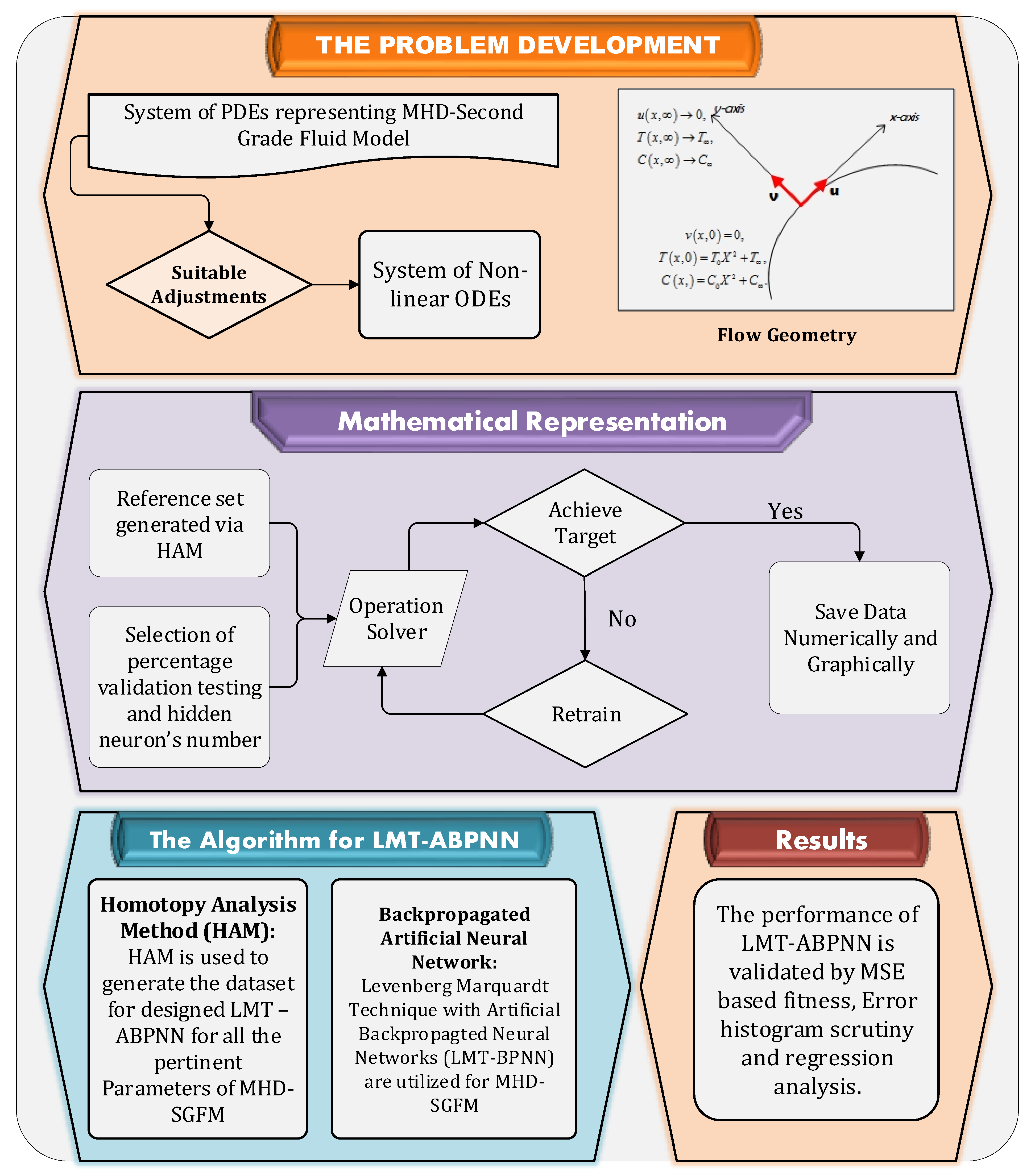
- An innovative application of Levenberg Marquardt Technique with artificial back propagated neural networks (LMT-ABPNN) is designed to examine the EOP in MHD-SGFM with Marangoni convection, Joule heating, and dissipation impact.
- Generating datasets through HAM and utilizing in training/validation/testing processes as targets to determine the approximated solution of proposed LMT-ABPNN.
- The suggested technique efficiently examines the dynamics of the problem for many scenarios based on the variation of pertinent parameters to depict flows, velocity, concentration, and temperature profiles.
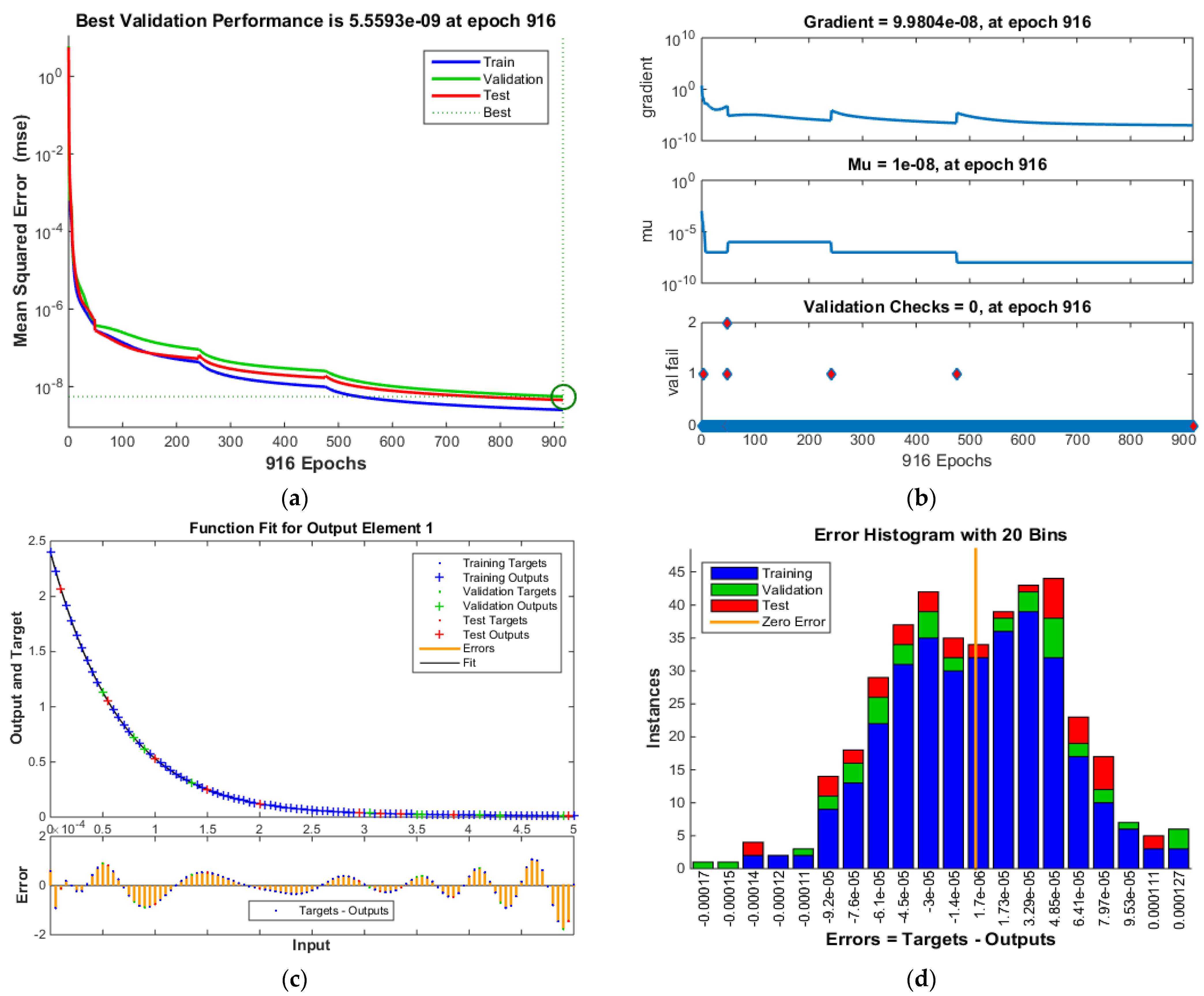
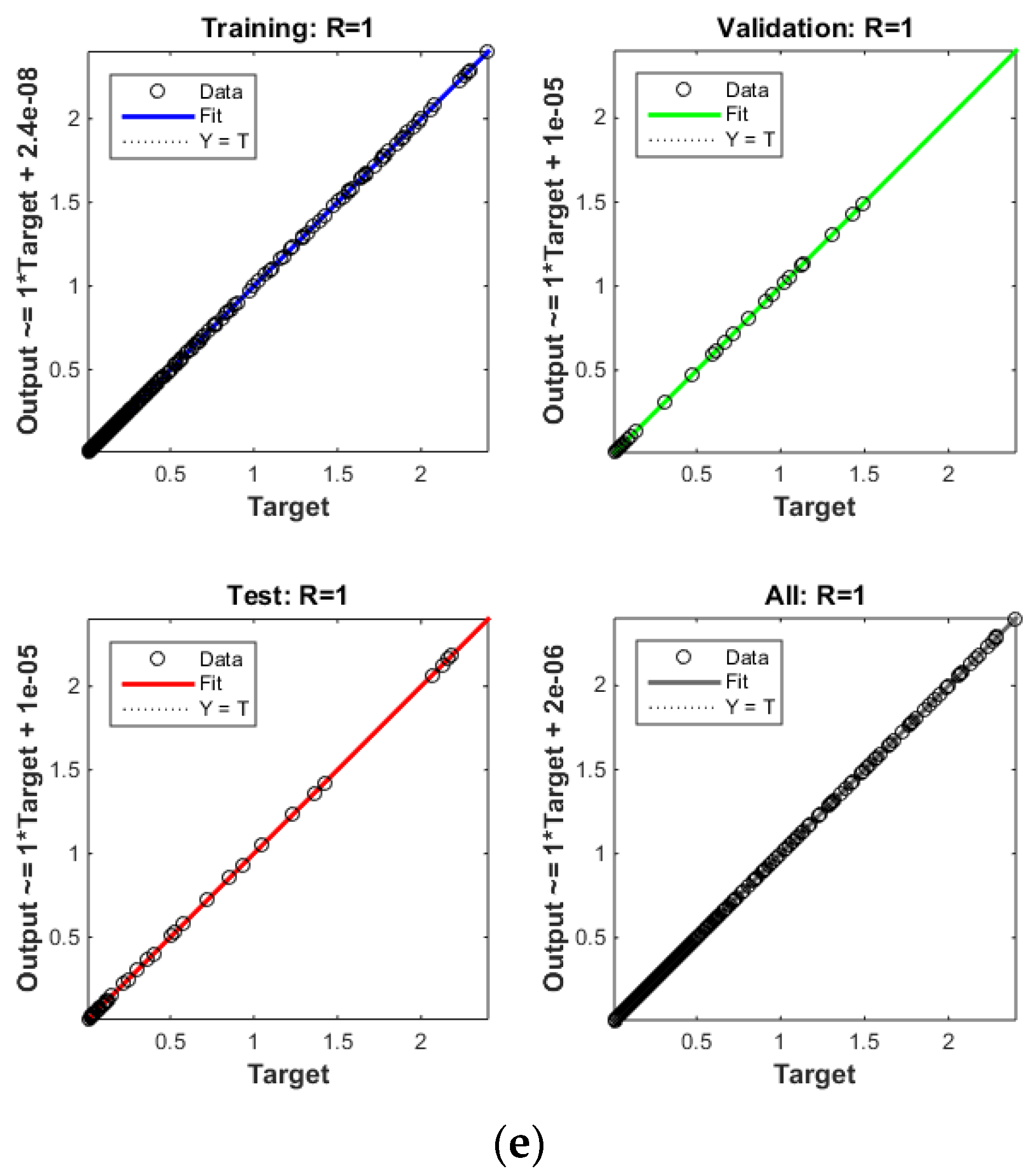
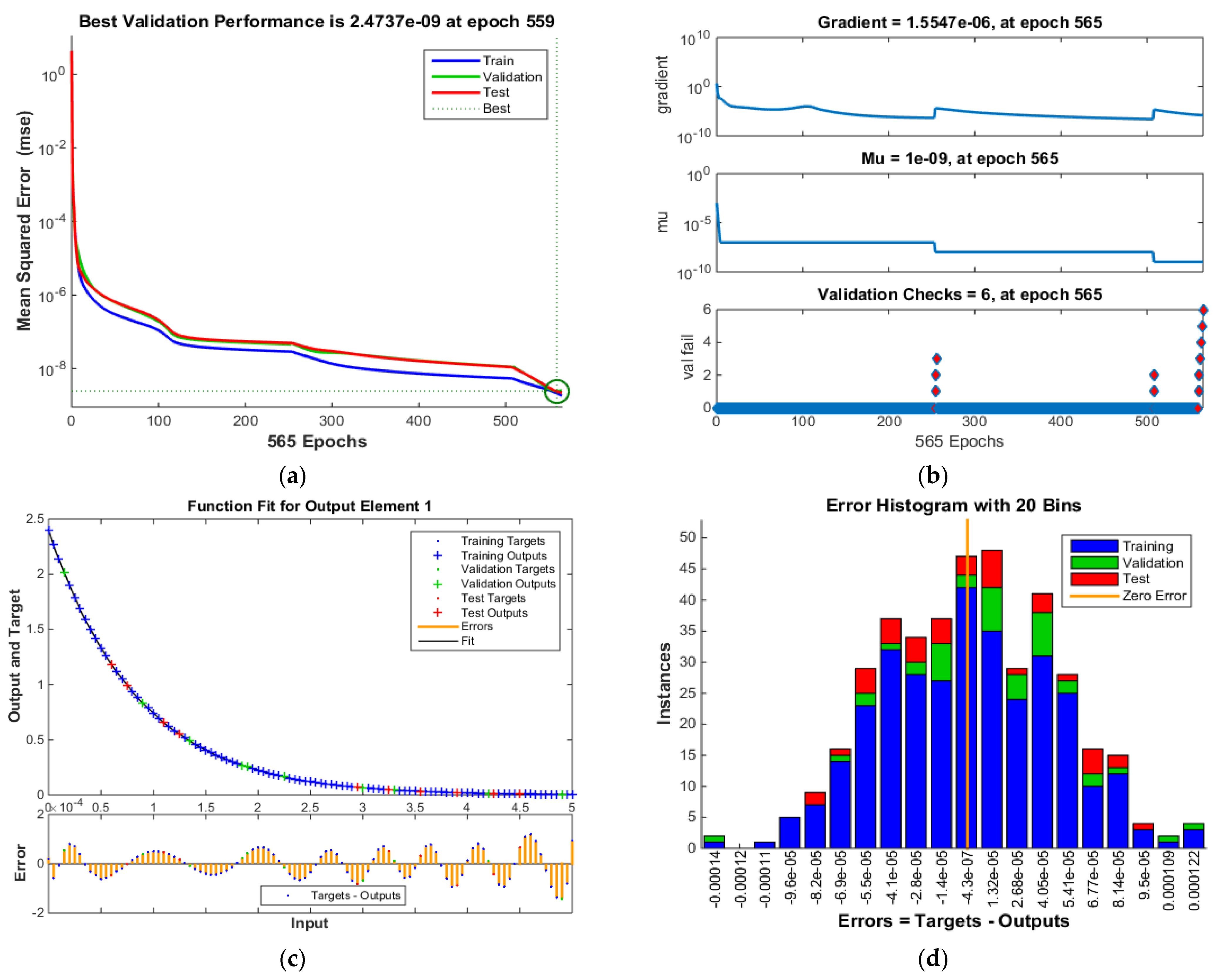
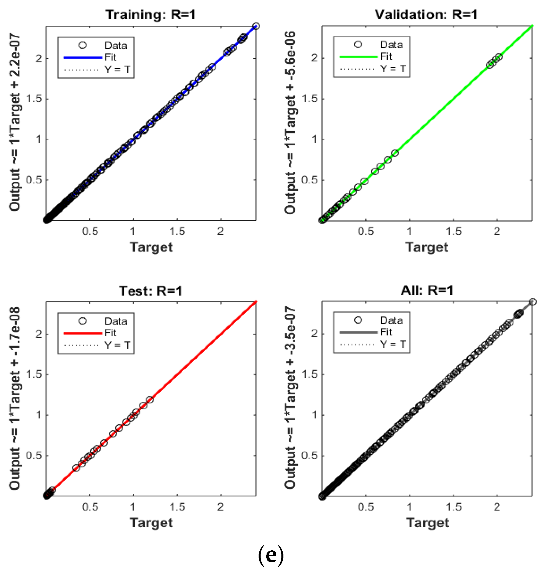
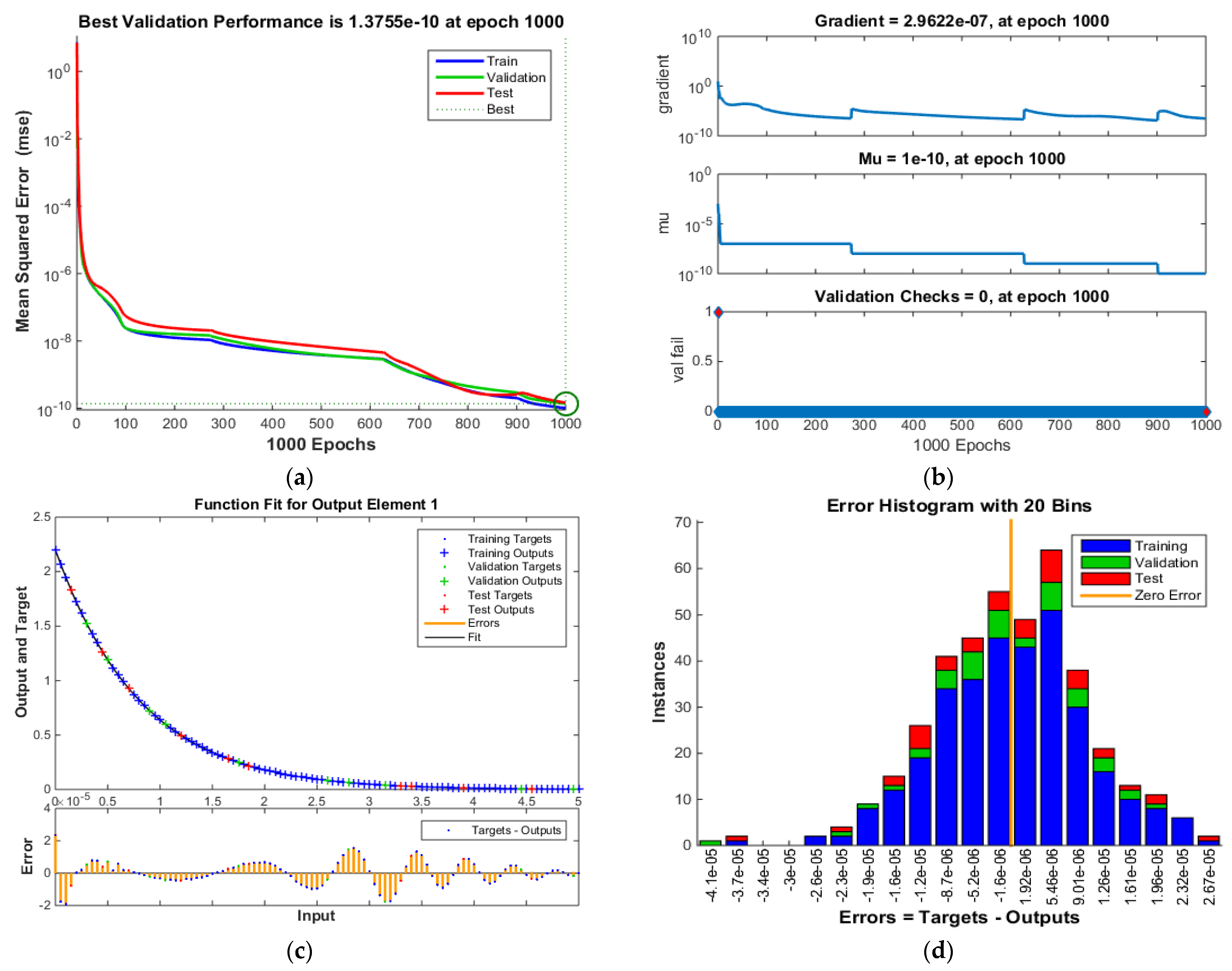
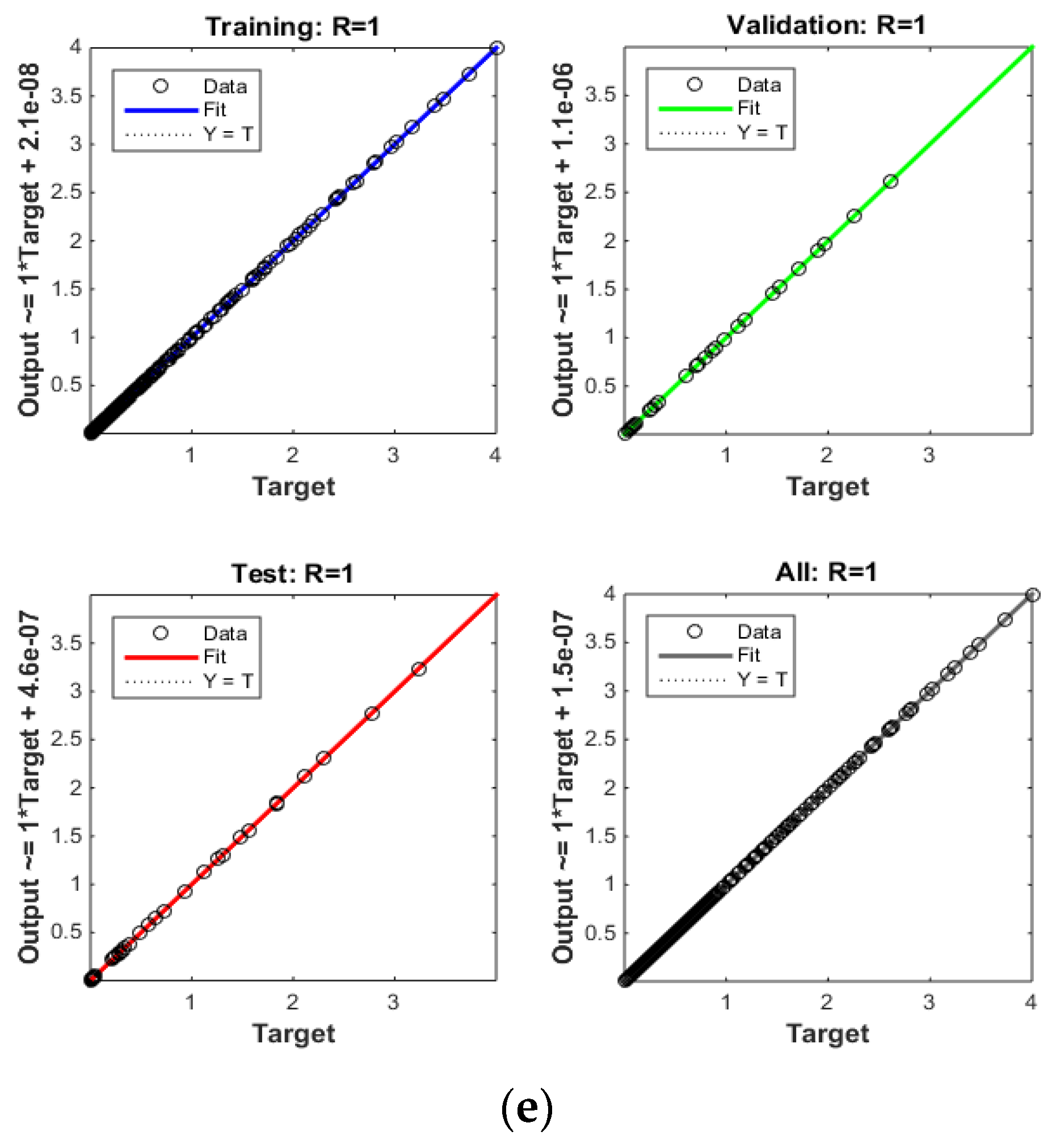
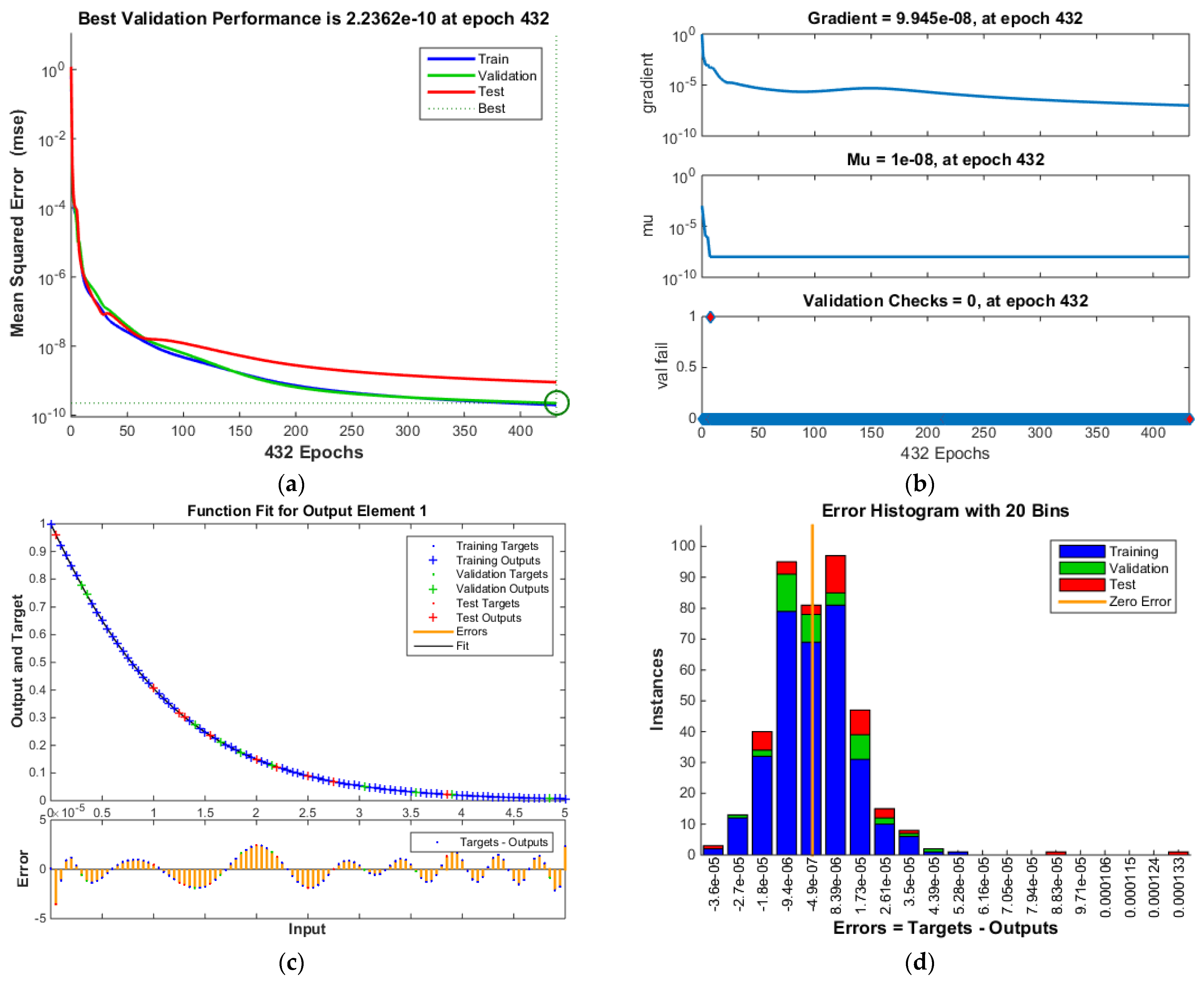
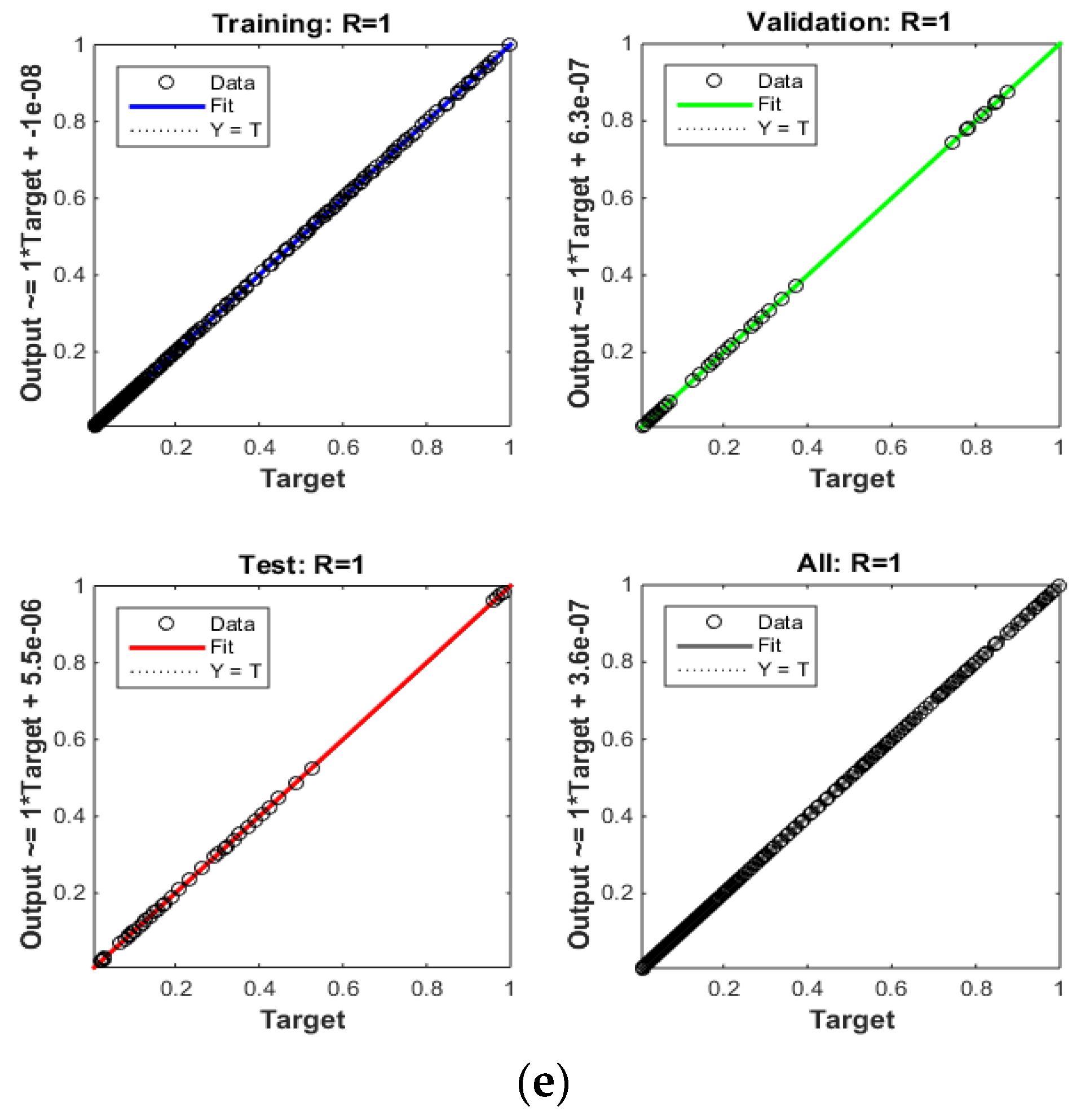
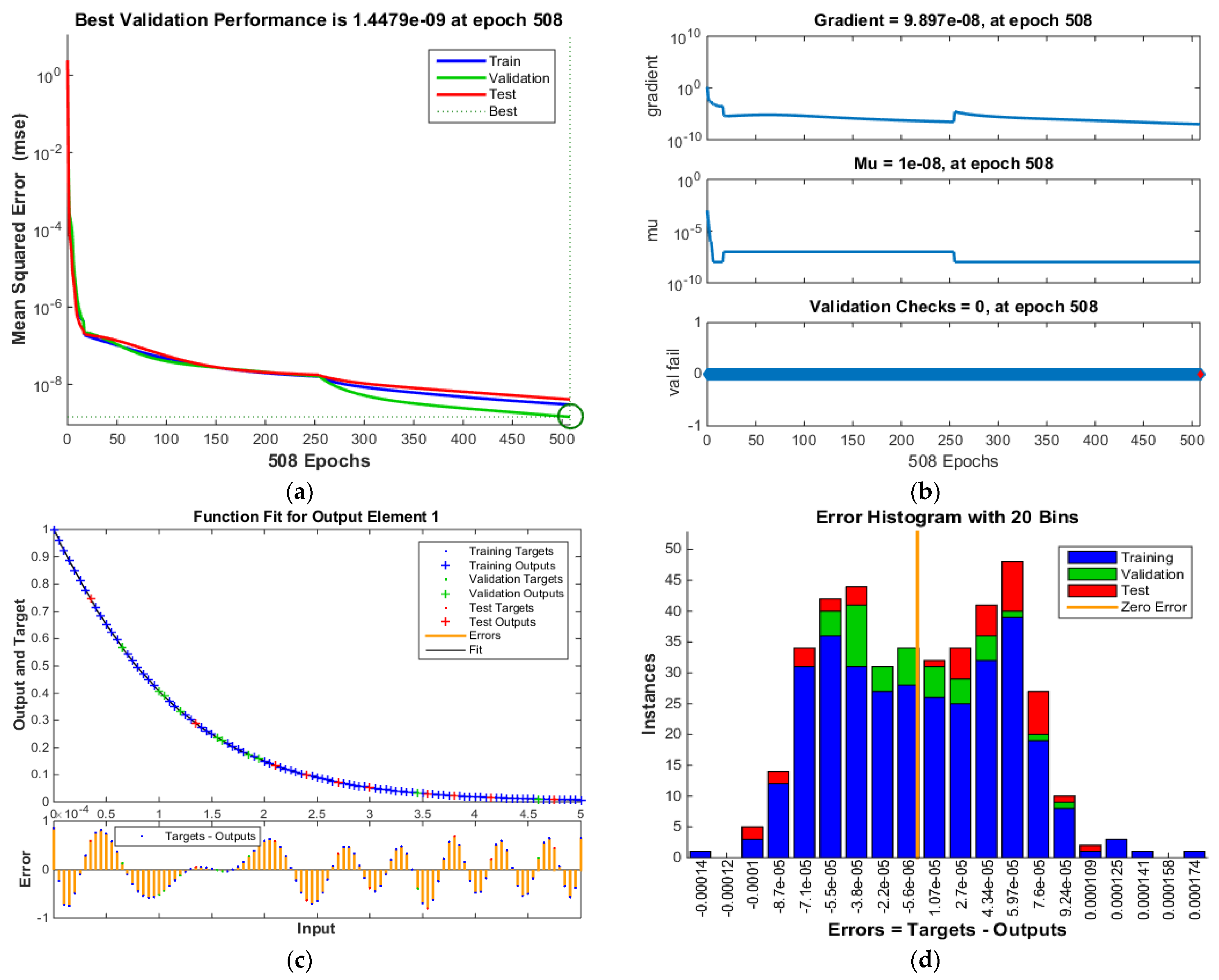
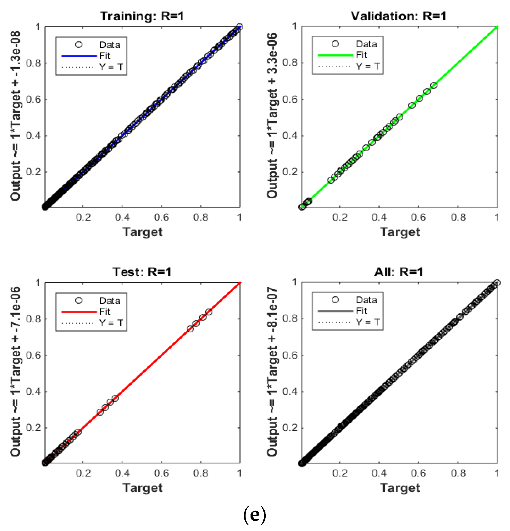
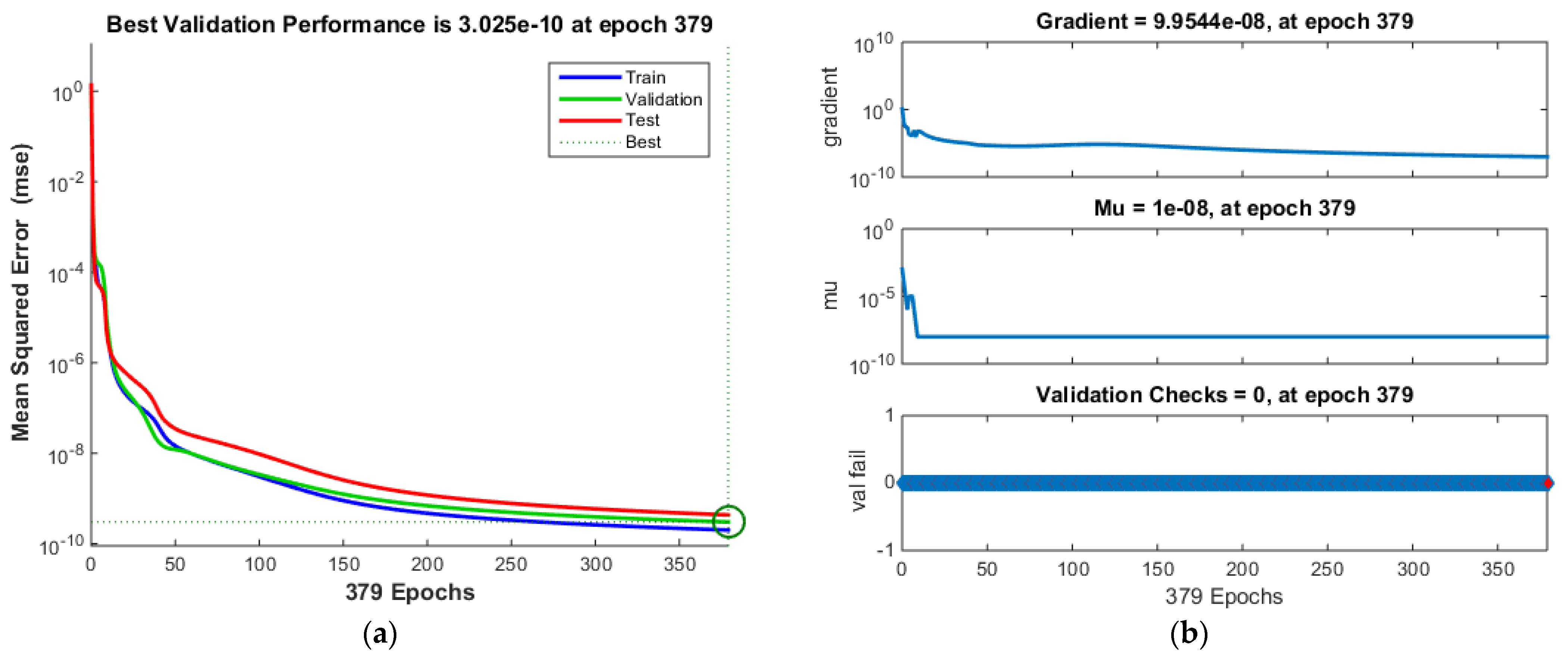
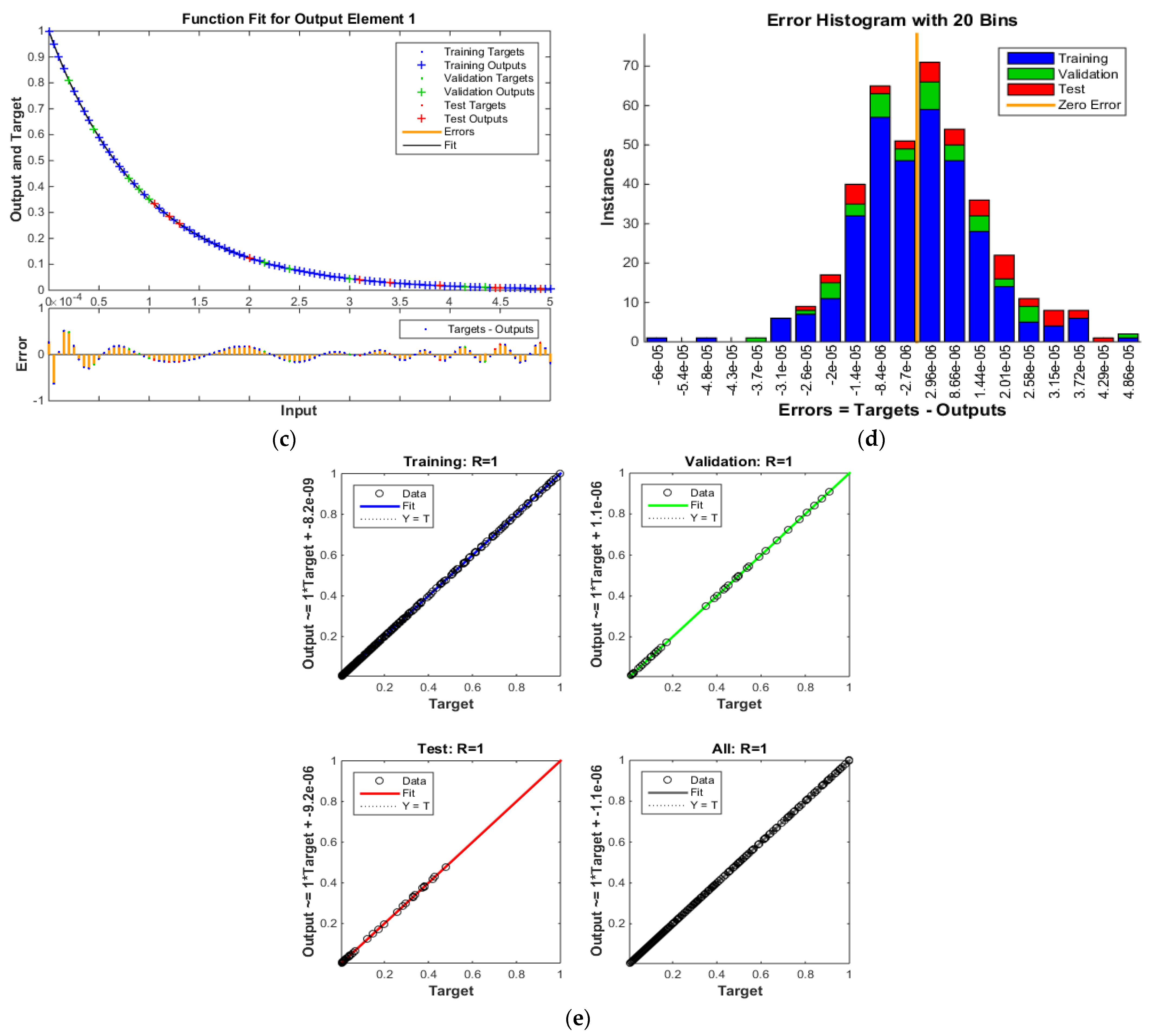
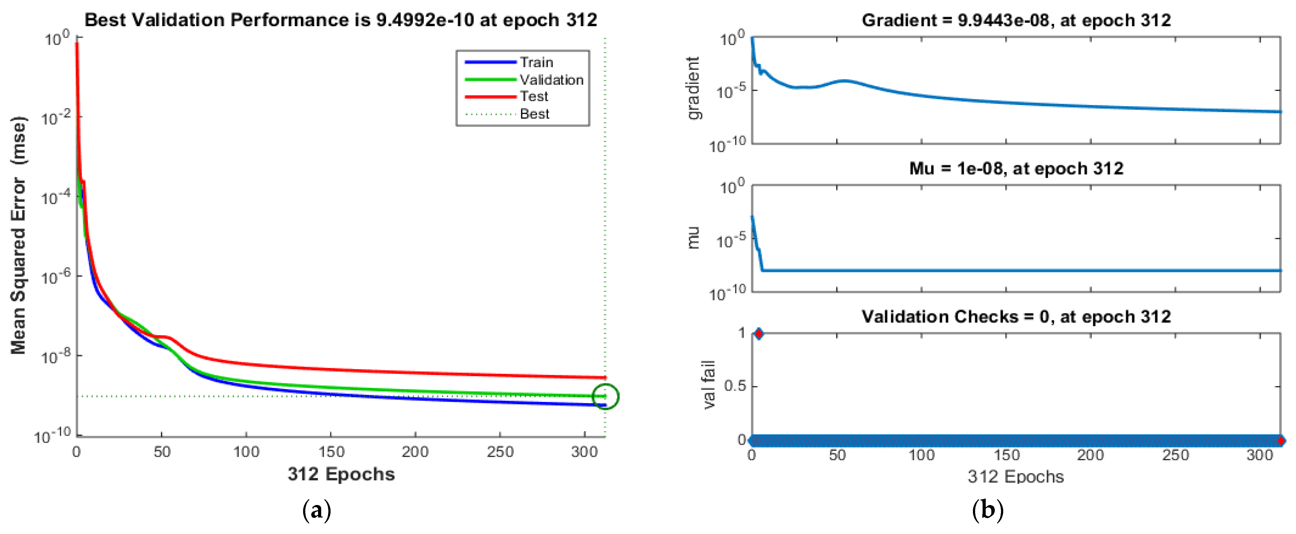
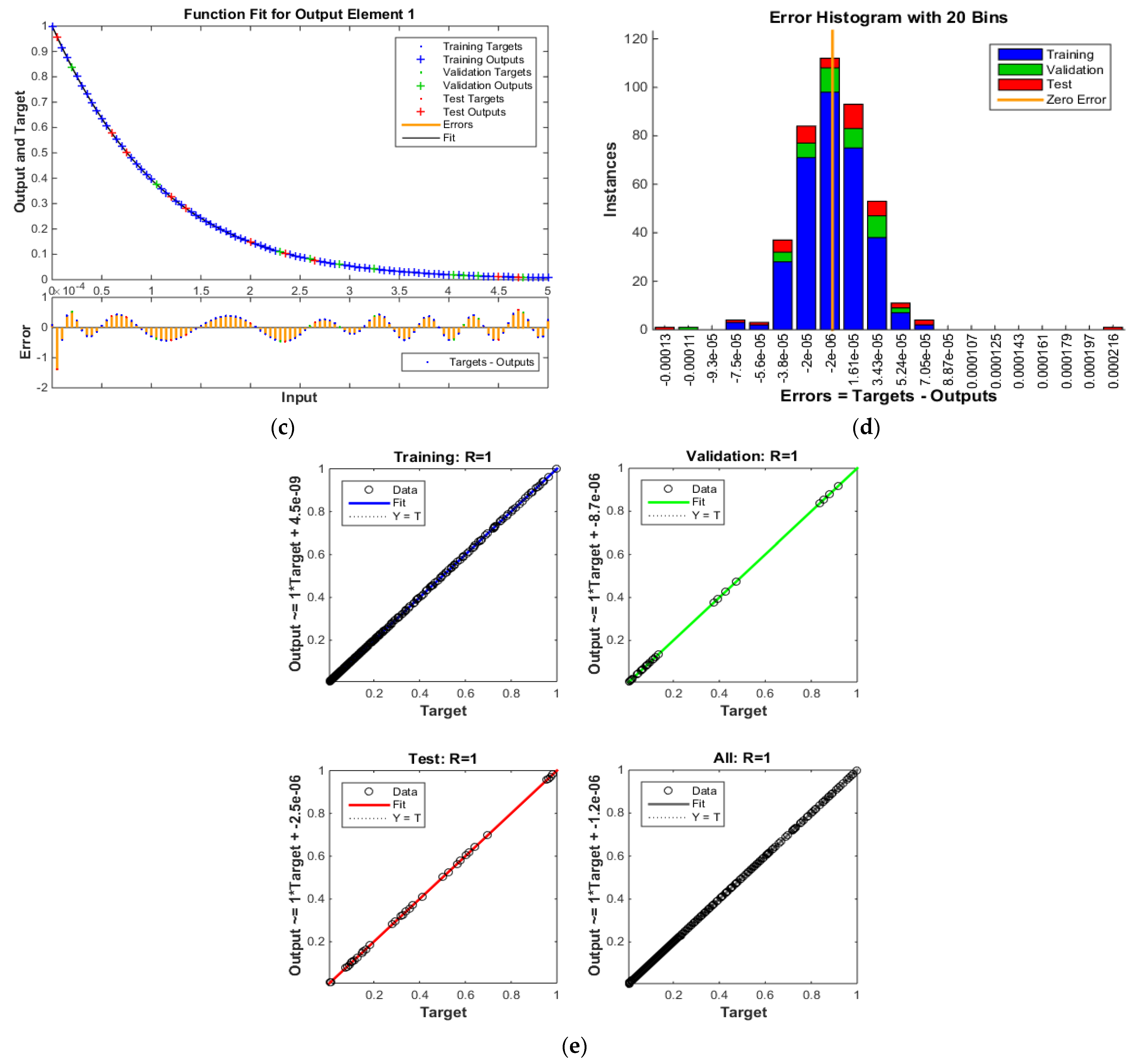
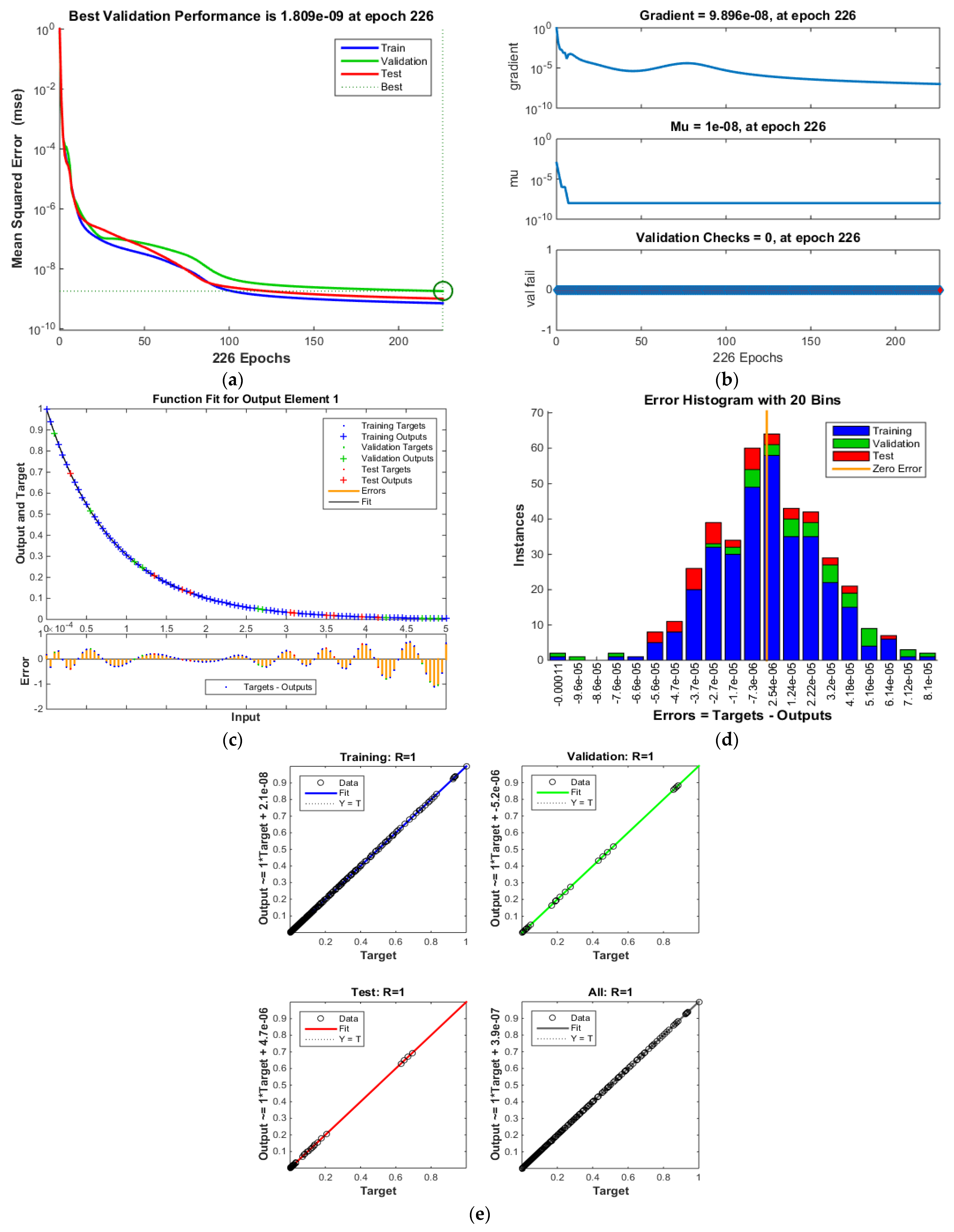
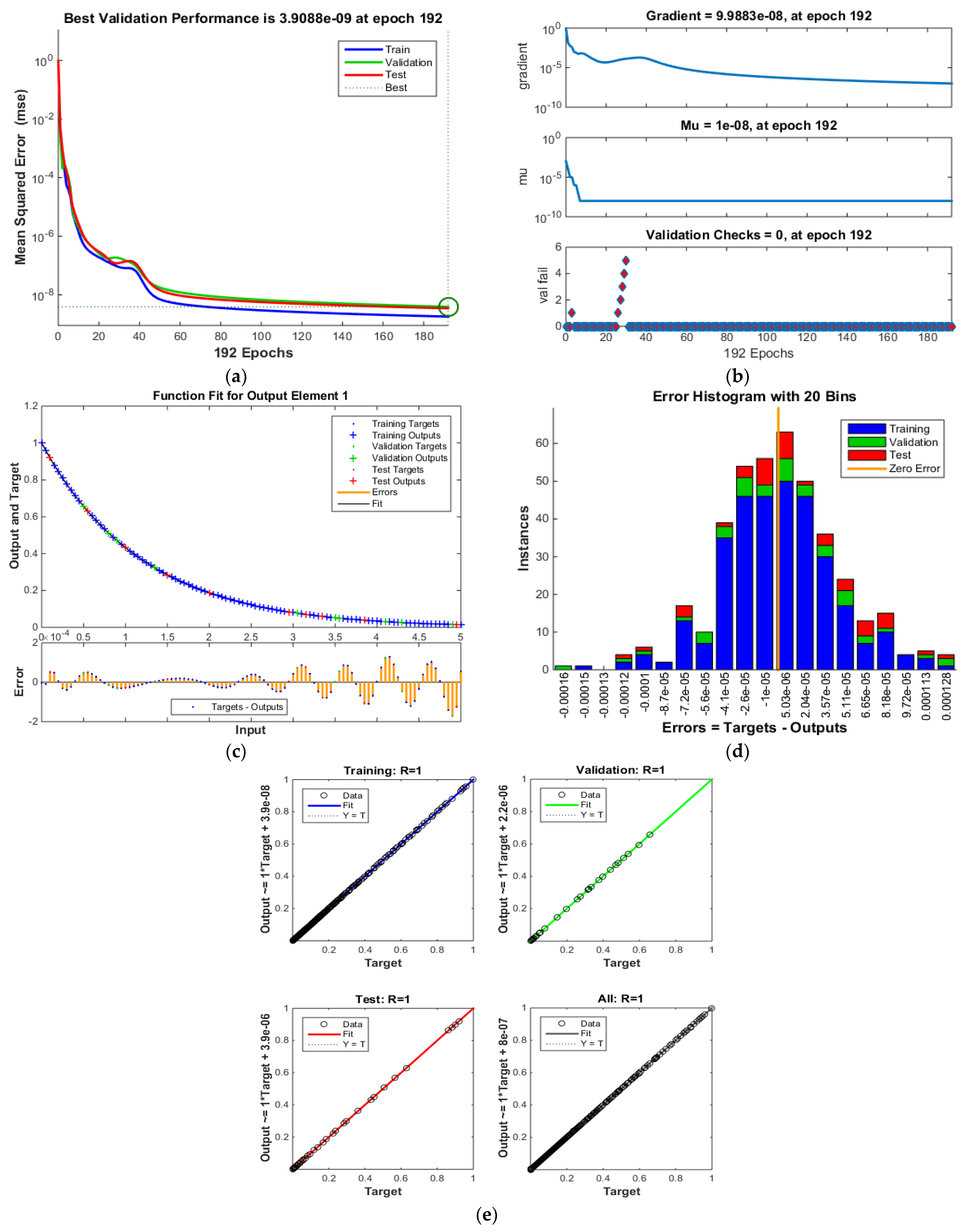
- The LMT-ABPNN’s validity and verification are based on a thorough examination of accuracy assessments, histograms, and regression analysis conducted for the MHD-SGFM, which are given graphically and numerically in sufficient detail.
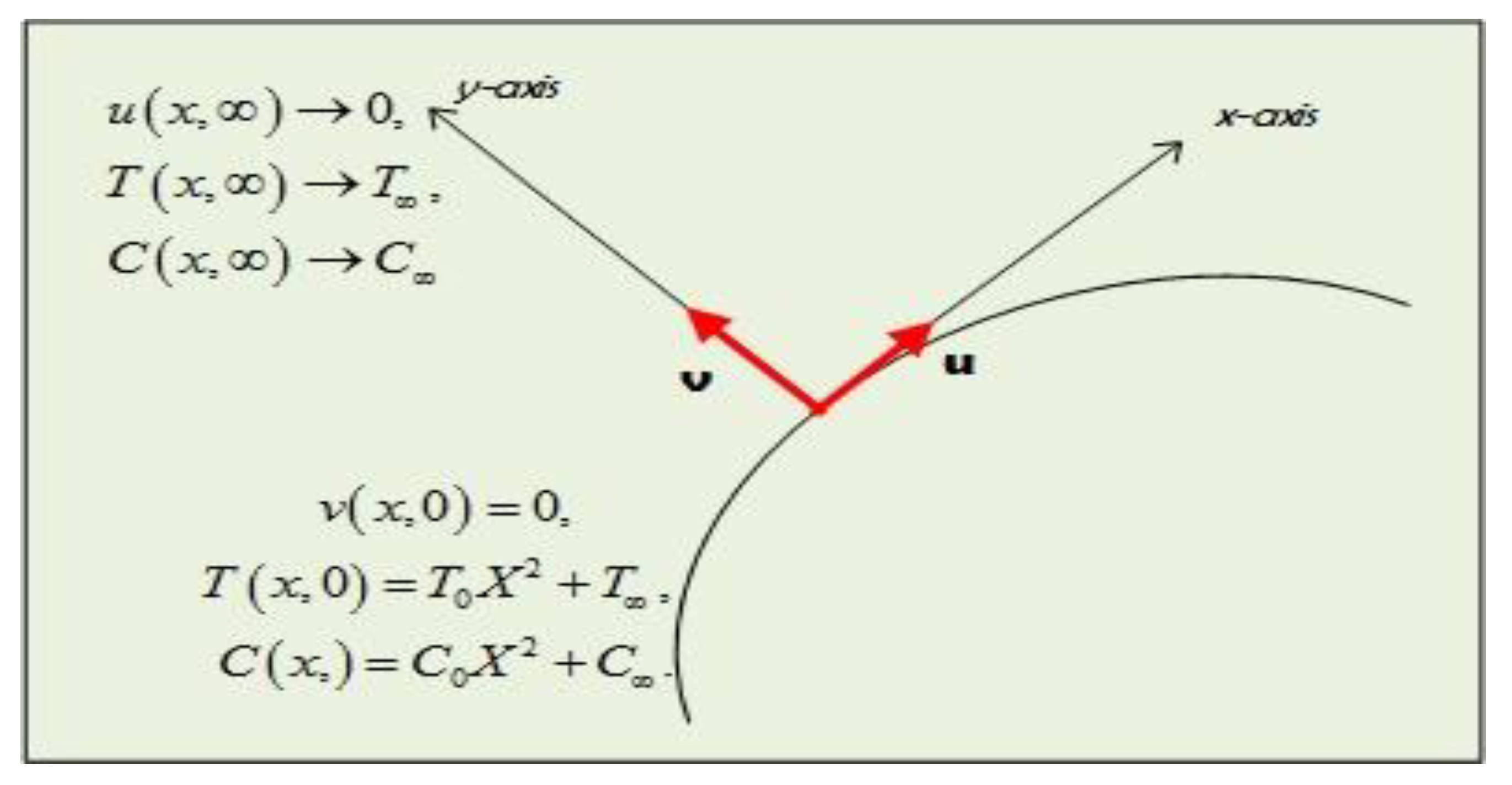
2. Problem Statement
Entropy Optimization
3. Solution Methodology
4. Result Interpretations
5. Impact of Profiles
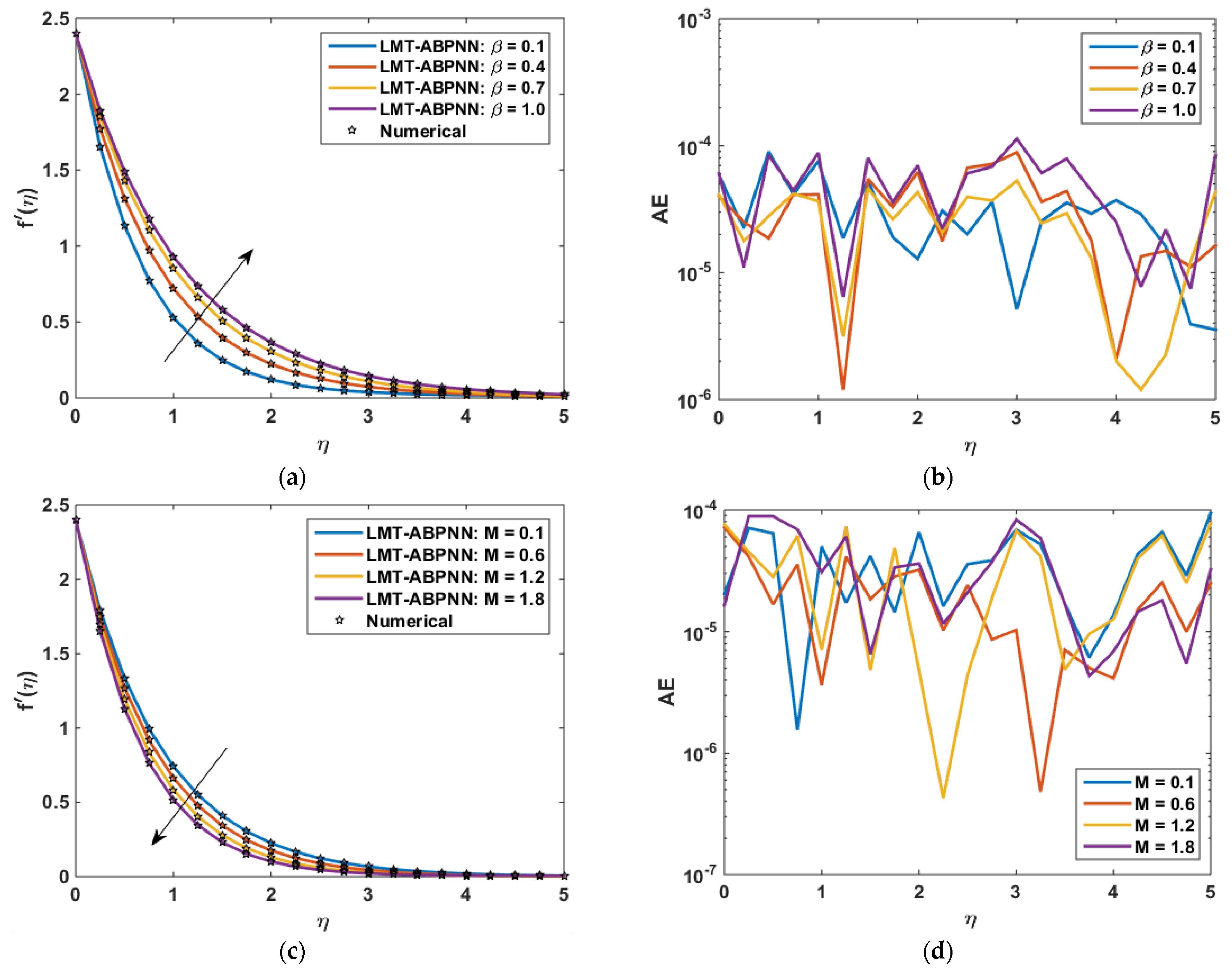
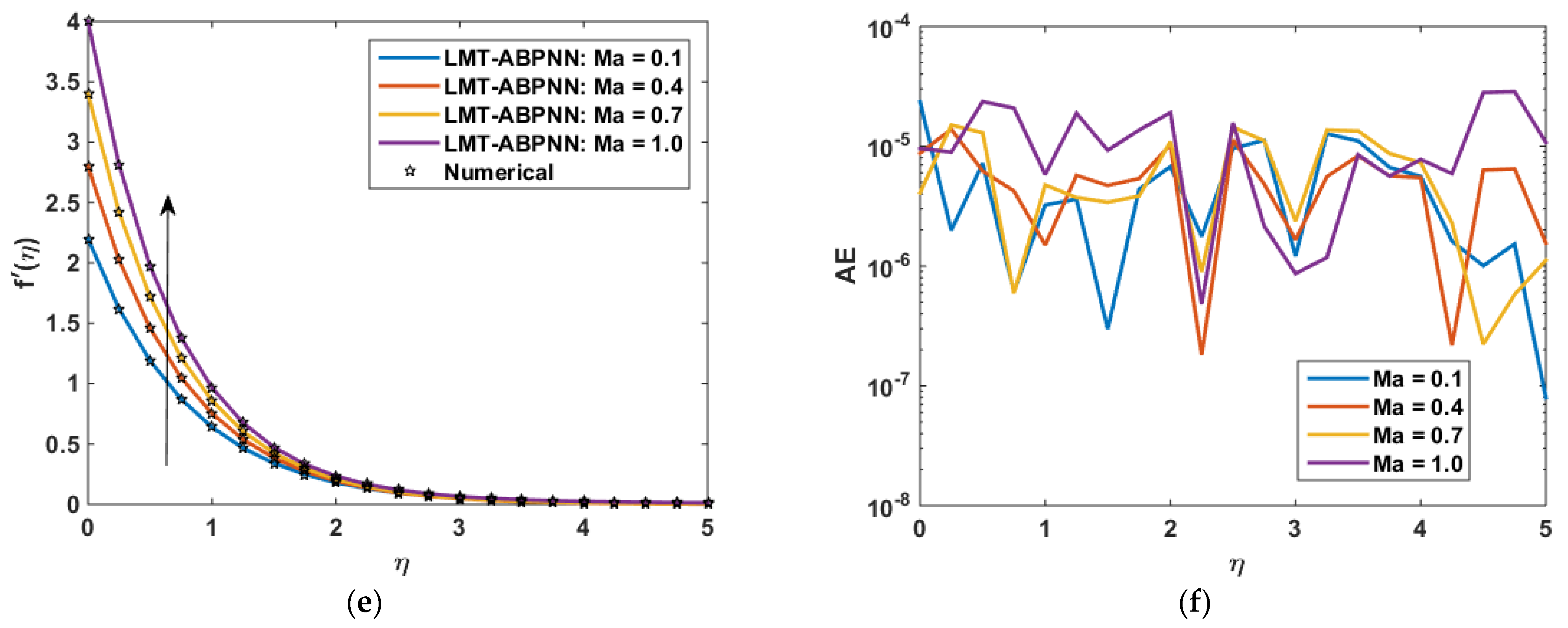
5.1. Influence on Velocity Gradient
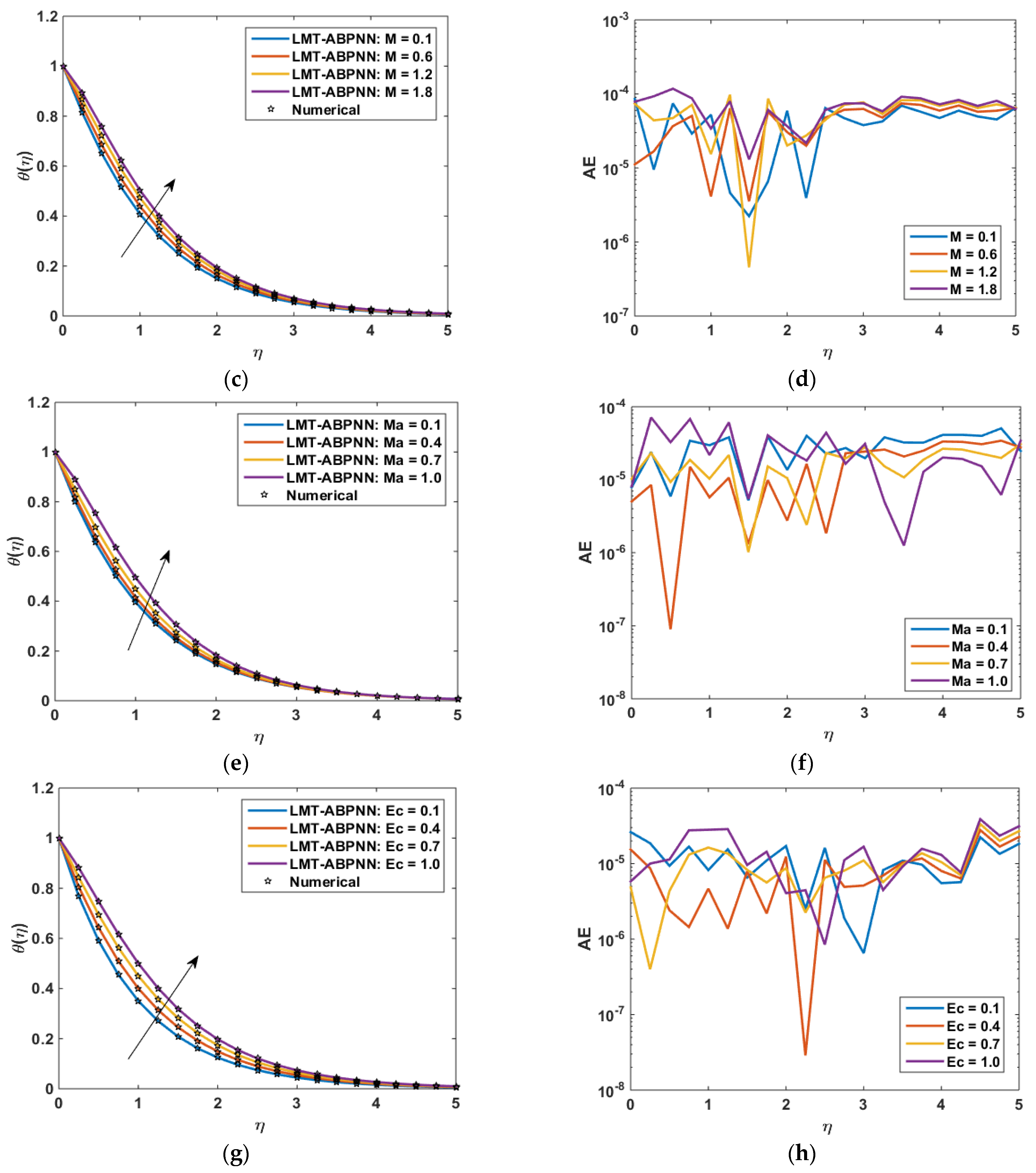
5.2. Influence on Temperature Gradient
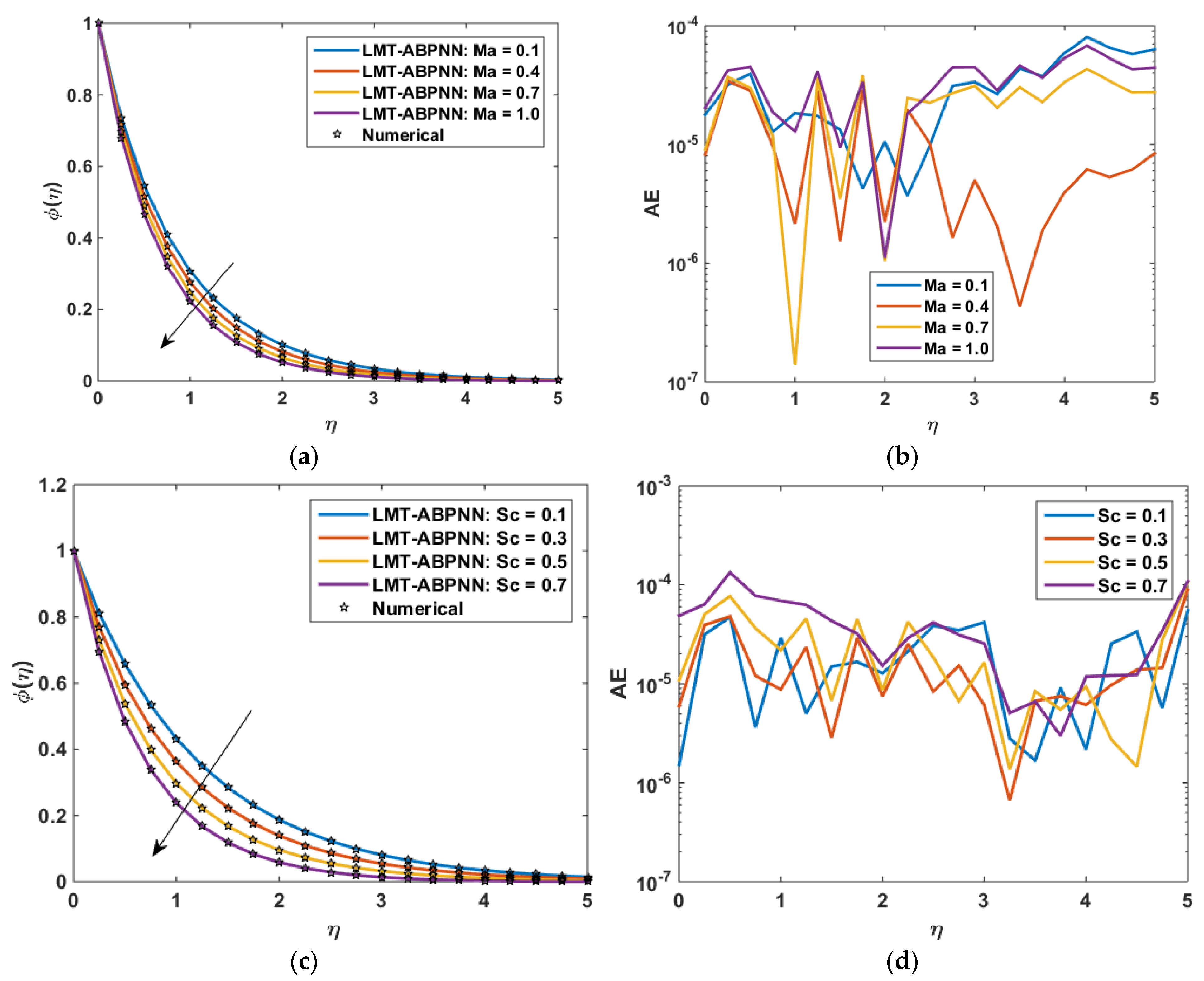
5.3. Influence on Concentration Field
5.4. Entropy Generation and Bejan Number Analysis
6. Conclusions
- The LMT-ABPNN’s validity and verification are based on a thorough examination of accuracy assessments, histograms, and regression analysis.
- The higher the network’s testing and training efficiency, the better the convergence of the produced results for the lowest Mu and gradient values.
- The larger , the higher while has the reverse influence on .
- For higher values of , boosts.
- The concentration drops as grow.
- An augmentation is noticed for for higher estimations of and
- Larger and decays the Bejan number.
Author Contributions
Funding
Institutional Review Board Statement
Informed Consent Statement
Data Availability Statement
Acknowledgments
Conflicts of Interest
Nomenclature
| Ambient concentration | Prandtl number | ||
| Ambient Temperature of fluid | Schmidt Number | ||
| Bejan number | Temperature of fluid | ||
| Brinkman Number | Thermal Conductivity | ||
| Cartesian co-ordinates | Velocity components | ||
| Concentration | Greek Symbol | ||
| Dimensionless Parameter | Density | ||
| Eckert number | Dynamic viscosity | ||
| Entropy optimization rate | Electric conductivity | ||
| Reference length | Positive constant | ||
| Magnetic strength | SG Fluid parameter | ||
| Marangoni ratio parameter | SG liquid parameter | ||
| Mass Diffusivity | Specific Heat | ||
References
- Pearson, J.R.A. On convection cells induced by surface tension. J. Fluid Mech. 1958, 4, 489–500. [Google Scholar] [CrossRef]
- Scriven, L.E.; Sternling, C.V. The marangoni effects. Nature 1960, 187, 186–188. [Google Scholar] [CrossRef]
- Qayyum, S. Dynamics of marangoni convection in hybrid nanofluid flow submerged in ethylene glycol and water base fluids. Int. Commun. Heat Mass Transf. 2020, 119, 104962. [Google Scholar] [CrossRef]
- Jawad, M.; Saeed, A.; Kumam, P.; Shah, Z.; Khan, A. Analysis of boundary layer MHD darcy-forchheimer radiative nanofluid flow with soret and dufour effects by means of marangoni convection. Case Stud. Therm. Eng. 2021, 23, 100792. [Google Scholar] [CrossRef]
- Gul, T.; Ullah, M.Z.; Alzahrani, A.K.; Zaheer, Z.; Amiri, I.S. MHD Thin film flow of kerosene oil based CNTs nanofluid under the influence of marangoni convection. Phys. Scr. 2020, 95, 015702. [Google Scholar] [CrossRef]
- Gul, T.; Akbar, R.; Zaheer, Z.; Amiri, I.S. The impact of the Marangoni convection and magnetic field versus blood-based carbon nanotube nanofluids. Proc. Inst. Mech. Eng. Part N J. Nanomater. Nanoeng. Nanosyst. 2020, 234, 37–46. [Google Scholar] [CrossRef]
- Rasool, G.; Shafiq, A.; Khalique, C.M. Marangoni forced convective casson type nanofluid flow in the presence of lorentz force generated by riga plate. Discret. Contin. Dyn. Syst. S 2021, 14, 2517. [Google Scholar] [CrossRef]
- Rasool, G.; Zhang, T.; Chamkha, A.J.; Shafiq, A.; Tlili, I.; Shahzadi, G. Entropy generation and consequences of binary chemical reaction on MHD Darcy–Forchheimer Williamson nanofluid flow over non-linearly stretching surface. Entropy 2020, 22, 18. [Google Scholar] [CrossRef] [PubMed] [Green Version]
- Modather, M.; Chamkha, A. An Analytical study of MHD heat and mass transfer oscillatory flow of a micropolar fluid over a vertical permeable plate in a porous medium. Turk. J. Eng. Environ. Sci. 2010, 33, 245–258. [Google Scholar]
- Krishna, M.V.; Chamkha, A.J. Hall and ion slip effects on MHD rotating boundary layer flow of nanofluid past an infinite vertical plate embedded in a porous medium. Results Phys. 2019, 15, 102652. [Google Scholar] [CrossRef]
- Chamkha, A.J.; Issa, C.; Khanafer, K. Natural convection from an inclined plate embedded in a variable porosity porous medium due to solar radiation. Int. J. Therm. Sci. 2002, 41, 73–81. [Google Scholar] [CrossRef]
- Chamkha, A.J. Non-darcy fully developed mixed convection in a porous medium channel with heat generation/absorption and hydromagnetic effects. Numer. Heat Transf. Part A Appl. 1997, 32, 653–675. [Google Scholar] [CrossRef]
- Takhar, H.S.; Chamkha, A.J.; Nath, G. MHD Flow over a moving plate in a rotating fluid with magnetic field, hall currents and free stream velocity. Int. J. Eng. Sci. 2002, 40, 1511–1527. [Google Scholar] [CrossRef]
- Takhar, H.S.; Chamkha, A.J.; Nath, G. Unsteady flow and heat transfer on a semi-infinite flat plate with an aligned magnetic field. Int. J. Eng. Sci. 1999, 37, 1723–1736. [Google Scholar] [CrossRef]
- Chamkha, A.J. Hydromagnetic three-dimensional free convection on a vertical stretching surface with heat generation or absorption. Int. J. Heat Fluid Flow 1999, 20, 84–92. [Google Scholar] [CrossRef]
- Ali, B.; Shafiq, A.; Siddique, I.; Al-Mdallal, Q.; Jarad, F. Significance of suction/injection, gravity modulation, thermal radiation, and magnetohydrodynamic on dynamics of micropolar fluid subject to an inclined sheet via finite element approach. Case Stud. Therm. Eng. 2021, 28, 101537. [Google Scholar] [CrossRef]
- Ali, B.; Thumma, T.; Habib, D.; Riaz, S. Finite element analysis on transient MHD 3D rotating flow of Maxwell and tangent hyperbolic nanofluid past a bidirectional stretching sheet with Cattaneo Christov heat flux model. Therm. Sci. Eng. Prog. 2021, 101089. (In press) [Google Scholar] [CrossRef]
- Ali, B.; Siddique, I.; Ahmadian, A.; Senu, N.; Ali, L.; Haider, A. Significance of Lorentz and Coriolis forces on dynamics of water based silver tiny particles via finite element simulation. Ain Shams Eng. J. 2021, in press. [Google Scholar] [CrossRef]
- Li, Y.X.; Qayyum, S.; Khan, M.I.; Elmasry, Y.; Chu, Y.M. Motion of hybrid nanofluid (MnZnFe2O4–NiZnFe2O4–H2O) with homogeneous–heterogeneous reaction: Marangoni convection. Math. Comput. Simul. 2021, 190, 1379–1391. [Google Scholar] [CrossRef]
- Khan, M.I.; Qayyum, S.; Shah, F.; Kumar, R.N.; Gowda, R.P.; Prasannakumara, B.C.; Chu, Y.M.; Kadry, S. Marangoni convective flow of hybrid nanofluid (MnZnFe2O4-NiZnFe2O4-H2O) with Darcy Forchheimer medium. Ain Shams Eng. J. 2021, 12, 3931–3938. [Google Scholar] [CrossRef]
- Khan, M.I.; Qayyum, S.; Chu, Y.M.; Khan, N.B.; Kadry, S. Transportation of marangoni convection and irregular heat source in entropy optimized dissipative flow. Int. Commun. Heat Mass Transf. 2021, 120, 105031. [Google Scholar] [CrossRef]
- Malaikah, H.; Ijaz Khan, M. Dynamics of Marangoni convection in radiative flow of power-law fluid with entropy optimization. Int. J. Mod. Phys. B 2021, 35, 2150280. [Google Scholar] [CrossRef]
- Ahmed, S.E.; Oztop, H.F.; Elshehabey, H.M. Thermosolutal Marangoni convection of bingham non-Newtonian fluids within inclined lid-driven enclosures full of porous media. Heat Transf. 2021, 50, 7898–7917. [Google Scholar] [CrossRef]
- Khan, M.I.; Qayyum, S.; Chu, Y.M.; Kadry, S. Numerical simulation and modeling of entropy generation in Marangoni convective flow of nanofluid with activation energy. Numer. Methods Partial. Differ. Equ. 2020, in press. [Google Scholar] [CrossRef]
- Khan, S.A.; Hayat, T.; Alsaedi, A.; Zai, Q.Z. Irreversibility analysis in Marangoni forced convection flow of second grade fluid. J. Phys. Commun. 2020, 4, 085013. [Google Scholar] [CrossRef]
- Abiodun, O.I.; Jantan, A.; Omolara, A.E.; Dada, K.V.; Mohamed, N.A.; Arshad, H. State-of-the-art in artificial neural network applications: A survey. Heliyon 2018, 4, e00938. [Google Scholar] [CrossRef] [Green Version]
- Bui, D.K.; Nguyen, T.N.; Ngo, T.D.; Nguyen-Xuan, H. An artificial neural network (ANN) expert system enhanced with the electromagnetism-based firefly algorithm (EFA) for predicting the energy consumption in buildings. Energy 2020, 190, 116370. [Google Scholar] [CrossRef]
- Zhao, Z.; Lou, Y.; Chen, Y.; Lin, H.; Li, R.; Yu, G. Prediction of interfacial interactions related with membrane fouling in a membrane bioreactor based on radial basis function artificial neural network (ANN). Bioresour. Technol. 2019, 282, 262–268. [Google Scholar] [CrossRef] [PubMed]
- Moayedi, H.; Mosallanezhad, M.; Rashid, A.S.A.; Jusoh, W.A.W.; Muazu, M.A. A systematic review and meta-analysis of artificial neural network application in geotechnical engineering: Theory and applications. Neural Comput. Appl. 2020, 32, 495–518. [Google Scholar] [CrossRef]
- Bukhari, A.H.; Sulaiman, M.; Islam, S.; Shoaib, M.; Kumam, P.; Raja, M.A.Z. Neuro-fuzzy modeling and prediction of summer precipitation with application to different meteorological stations. Alex. Eng. J. 2020, 59, 101–116. [Google Scholar] [CrossRef]
- Xia, M.; Zheng, X.; Imran, M.; Shoaib, M. Data-driven prognosis method using hybrid deep recurrent neural network. Appl. Soft Comput. 2020, 93, 106351. [Google Scholar] [CrossRef]
- Khan, R.A.; Ullah, H.; Raja, M.A.Z.; Khan, M.A.R.; Islam, S.; Shoaib, M. Heat transfer between two porous parallel plates of steady nano fludis with Brownian and thermophoretic effects: A new stochastic numerical approach. Int. Commun. Heat Mass Transf. 2021, 126, 105436. [Google Scholar] [CrossRef]
- Aljohani, J.L.; Alaidarous, E.S.; Raja, M.A.Z.; Shoaib, M.; Alhothuali, M.S. Intelligent computing through neural networks for numerical treatment of non-Newtonian wire coating analysis model. Sci. Rep. 2021, 11, 9072. [Google Scholar] [CrossRef]
- Shah, Z.; Raja, M.A.Z.; Chu, Y.M.; Khan, W.A.; Abbas, S.Z.; Shoaib, M.; Irfan, M. Computational intelligence of Levenberg-Marquardt backpropagation neural networks to study the dynamics of expanding/contracting cylinder for cross magneto-nanofluid flow model. Phys. Scr. 2021, 96, 055219. [Google Scholar] [CrossRef]
- Shoaib, M.; Raja, M.A.Z.; Jamshed, W.; Nisar, K.S.; Khan, I.; Farhat, I. Intelligent computing Levenberg Marquardt approach for entropy optimized single-phase comparative study of second grade nanofluidic system. Int. Commun. Heat Mass Transf. 2021, 127, 105544. [Google Scholar] [CrossRef]
- Raja, M.A.Z.; Shoaib, M.; Tabassum, R.; Khan, M.I.; Gowda, R.P.; Prasannakumara, B.C.; Malik, M.Y.; Xia, W.F. Intelligent computing for the dynamics of entropy optimized nanofluidic system under impacts of MHD along thick surface. Int. J. Mod. Phys. B 2021, 35, 2150269. [Google Scholar] [CrossRef]
- Raja, M.A.Z.; Shoaib, M.; Khan, Z.; Zuhra, S.; Saleel, C.A.; Nisar, K.S.; Islam, S.; Khan, I. Supervised neural networks learning algorithm for three dimensional hybrid nanofluid flow with radiative heat and mass fluxes. Ain Shams Eng. J. 2021, in press. [Google Scholar] [CrossRef]
- Ilyas, H.; Ahmad, I.; Raja, M.A.Z.; Tahir, M.B.; Shoaib, M. Neuro-intelligent mappings of hybrid hydro-nanofluid Al2O3–Cu–H2O model in porous medium over rotating disk with viscous dissolution and JOULE heating. Int. J. Hydrog. Energy 2021, 46, 28298–28326. [Google Scholar] [CrossRef]
- Ullah, H.; Khan, I.; Fiza, M.; Hamadneh, N.N.; Fayz-Al-Asad, M.; Islam, S.; Khan, I.; Raja, M.A.Z.; Shoaib, M. MHD boundary layer flow over a stretching sheet: A new stochastic method. Math. Probl. Eng. 2021, 2021, 9924593. [Google Scholar] [CrossRef]
- Ahmad, I.; Ilyas, H.; Raja, M.A.Z.; Khan, Z.; Shoaib, M. Stochastic numerical computing with Levenberg–Marquardt backpropagation for performance analysis of heat sink of functionally graded material of the porous fin. Surf. Interfaces 2021, 26, 101403. [Google Scholar] [CrossRef]
- Khan, I.; Ullah, H.; AlSalman, H.; Fiza, M.; Islam, S.; Zahoor Raja, A.; Shoaib, M.; Gumaei, A.H. Falkner–Skan equation with heat transfer: A new stochastic numerical approach. Math. Probl. Eng. 2021, 2021, 3921481. [Google Scholar] [CrossRef]
- Umar, M.; Sabir, Z.; Raja, M.A.Z.; Aguilar, J.G.; Amin, F.; Shoaib, M. Neuro-swarm intelligent computing paradigm for nonlinear HIV infection model with CD4+ T-cells. Math. Comput. Simul. 2021, 188, 241–253. [Google Scholar] [CrossRef]
- Sabir, Z.; Raja, M.A.Z.; Guirao, J.L.; Saeed, T. Meyer Wavelet neural networks to solve a novel design of fractional order pantograph lane-emden differential model. Chaos Solitons Fractals 2021, 152, 111404. [Google Scholar] [CrossRef]
- Ali, W.; Li, Y.; Raja, M.A.Z.; Khan, W.U.; He, Y. State estimation of an underwater markov chain maneuvering target using intelligent computing. Entropy 2021, 23, 1124. [Google Scholar] [CrossRef] [PubMed]
- Shercliff, J.A. Textbook of Magnetohydrodynamics; Pergamon Press: Oxford, UK, 1965. [Google Scholar]
- Cramer, K.R.; Pai, S.I. Magnetofluid Dynamics for Engineers and Applied Physicists; McGrawhill: New York, NY, USA, 1973. [Google Scholar]
- Hayat, T.; Khan, S.A.; Alsaedi, A. Simulation and modeling of entropy optimized MHD flow of second grade fluid with dissipation effect. J. Mater. Res. Technol. 2020, 9, 11993–12006. [Google Scholar] [CrossRef]
- Magyari, E.; Chamkha, A.J. Exact analytical results for the thermosolutal MHD Marangoni boundary layers. Int. J. Therm. Sci. 2008, 47, 848–857. [Google Scholar] [CrossRef]
- Sheikholeslami, M.; Chamkha, A.J. Influence of Lorentz forces on nanofluid forced convection considering Marangoni convection. J. Mol. Liq. 2017, 225, 750–757. [Google Scholar] [CrossRef]
- Shoaib, M.; Akhtar, R.; Khan, M.A.R.; Rana, M.A.; Siddiqui, A.M.; Zhiyu, Z.; Raja, M.A.Z. A novel design of three-dimensional mhd flow of second-grade fluid past a porous plate. Math. Probl. Eng. 2019, 2019, 2584397. [Google Scholar] [CrossRef] [Green Version]
- Shoaib, M.; Rana, M.A.; Siddiqui, A.M. The effect of slip condition on the three-dimensional flow of Jeffrey fluid along a plane wall with periodic suction. J. Braz. Soc. Mech. Sci. Eng. 2017, 39, 2495–2503. [Google Scholar] [CrossRef]
- Siddiqui, A.M.; Shoaib, M.; Rana, M.A. Three-dimensional flow of Jeffrey fluid along an infinite plane wall with periodic suction. Meccanica 2017, 52, 2705–2714. [Google Scholar] [CrossRef]
- Awais, M.; Raja, M.A.Z.; Awan, S.E.; Shoaib, M.; Ali, H.M. Heat and mass transfer phenomenon for the dynamics of casson fluid through porous medium over shrinking wall subject to Lorentz force and heat source/sink. Alex. Eng. J. 2021, 60, 1355–1363. [Google Scholar] [CrossRef]


| Scenario | Fluid Variants | Case (1) | Case (2) | Case (3) | Case (4) |
|---|---|---|---|---|---|
| 1 | 0.1 | 0.4 | 0.7 | 1.0 | |
| 2 | 0.1 | 0.6 | 1.2 | 1.8 | |
| 3 | Ma | 0.1 | 0.4 | 0.7 | 1.0 |
| 4 | Ec | 0.1 | 0.4 | 0.7 | 1.0 |
| 5 | Sc | 0.1 | 0.3 | 0.5 | 0.7 |
| Physical Quantities | MSE | Performance | Grad | Mu | Epochs | Time | ||
|---|---|---|---|---|---|---|---|---|
| Training | Validation | Testing | ||||||
| 2.52 × 10⁻⁹ | 5.56 × 10⁻⁹ | 4.53 × 10⁻⁹ | 2.52 × 10⁻⁹ | 9.98 × 10⁻⁸ | 1.00 × 10⁻⁸ | 916 | 34 s | |
| M | 2.14 × 10⁻⁹ | 2.47 × 10⁻⁹ | 2.41 × 10⁻⁹ | 1.83 × 10⁻⁹ | 1.55 × 10⁻⁶ | 1.00 × 10⁻⁹ | 565 | 11 s |
| Ma | 1.01 × 10⁻¹⁰ | 1.38 × 10⁻¹⁰ | 1.46 × 10⁻¹⁰ | 1.01 × 10⁻¹⁰ | 2.96 × 10⁻⁷ | 1.00 × 10⁻¹⁰ | 1000 | 32 s |
| Physical Quantities | MSE | Performance | Grad | Mu | Epochs | Time | ||
|---|---|---|---|---|---|---|---|---|
| Training | Validation | Testing | ||||||
| 1.99 × 10⁻¹⁰ | 2.24 × 10⁻¹⁰ | 9.02 × 10⁻¹⁰ | 1.99 × 10⁻¹⁰ | 9.95 × 10⁻⁸ | 1.00 × 10⁻⁸ | 432 | 10 s | |
| M | 2.99 × 10⁻⁹ | 1.45 × 10⁻⁹ | 4.09 × 10⁻⁹ | 2.99 × 10⁻⁹ | 9.90 × 10⁻⁸ | 1.00 × 10⁻⁸ | 508 | 24 s |
| Ma | 5.69 × 10⁻¹⁰ | 9.50 × 10⁻¹⁰ | 2.79 × 10⁻⁹ | 5.69 × 10⁻¹⁰ | 9.94 × 10⁻⁸ | 1.00 × 10⁻⁸ | 312 | 9 s |
| Ec | 2.01 × 10⁻¹⁰ | 3.03 × 10⁻¹⁰ | 4.34 × 10⁻¹⁰ | 2.01 × 10⁻¹⁰ | 9.95 × 10⁻⁸ | 1.00 × 10⁻⁸ | 379 | 14 s |
| Physical Quantities | MSE | Performance | Grad | Mu | Epochs | Time | ||
|---|---|---|---|---|---|---|---|---|
| Training | Validation | Testing | ||||||
| Ma | 7.13 × 10⁻¹⁰ | 1.81 × 10⁻⁹ | 1.01 × 10⁻⁹ | 7.13 × 10⁻¹⁰ | 9.90 × 10⁻⁸ | 1.00 × 10⁻⁸ | 226 | 8 s |
| Sc | 1.81 × 10⁻⁹ | 3.91 × 10⁻⁹ | 3.47 × 10⁻⁹ | 1.81 × 10⁻⁹ | 9.99 × 10⁻⁸ | 1.00 × 10⁻⁸ | 192 | 6 s |
Publisher’s Note: MDPI stays neutral with regard to jurisdictional claims in published maps and institutional affiliations. |
© 2021 by the authors. Licensee MDPI, Basel, Switzerland. This article is an open access article distributed under the terms and conditions of the Creative Commons Attribution (CC BY) license (https://creativecommons.org/licenses/by/4.0/).
Share and Cite
Shoaib, M.; Tabassum, R.; Nisar, K.S.; Raja, M.A.Z.; Rafiq, A.; Khan, M.I.; Jamshed, W.; Abdel-Aty, A.-H.; Yahia, I.S.; E. Mahmoud, E. Entropy Optimized Second Grade Fluid with MHD and Marangoni Convection Impacts: An Intelligent Neuro-Computing Paradigm. Coatings 2021, 11, 1492. https://doi.org/10.3390/coatings11121492
Shoaib M, Tabassum R, Nisar KS, Raja MAZ, Rafiq A, Khan MI, Jamshed W, Abdel-Aty A-H, Yahia IS, E. Mahmoud E. Entropy Optimized Second Grade Fluid with MHD and Marangoni Convection Impacts: An Intelligent Neuro-Computing Paradigm. Coatings. 2021; 11(12):1492. https://doi.org/10.3390/coatings11121492
Chicago/Turabian StyleShoaib, Muhammad, Rafia Tabassum, Kottakkaran Sooppy Nisar, Muhammad Asif Zahoor Raja, Ayesha Rafiq, Muhammad Ijaz Khan, Wasim Jamshed, Abdel-Haleem Abdel-Aty, I. S. Yahia, and Emad E. Mahmoud. 2021. "Entropy Optimized Second Grade Fluid with MHD and Marangoni Convection Impacts: An Intelligent Neuro-Computing Paradigm" Coatings 11, no. 12: 1492. https://doi.org/10.3390/coatings11121492