
Comparative Numerical Study of Thermal Features Analysis between Oldroyd-B Copper and Molybdenum Disulfide Nanoparticles in Engine-Oil-Based Nanofluids Flow


 ,
,  , , , ,
  ,
,  and
and
Abstract
:1. Introduction
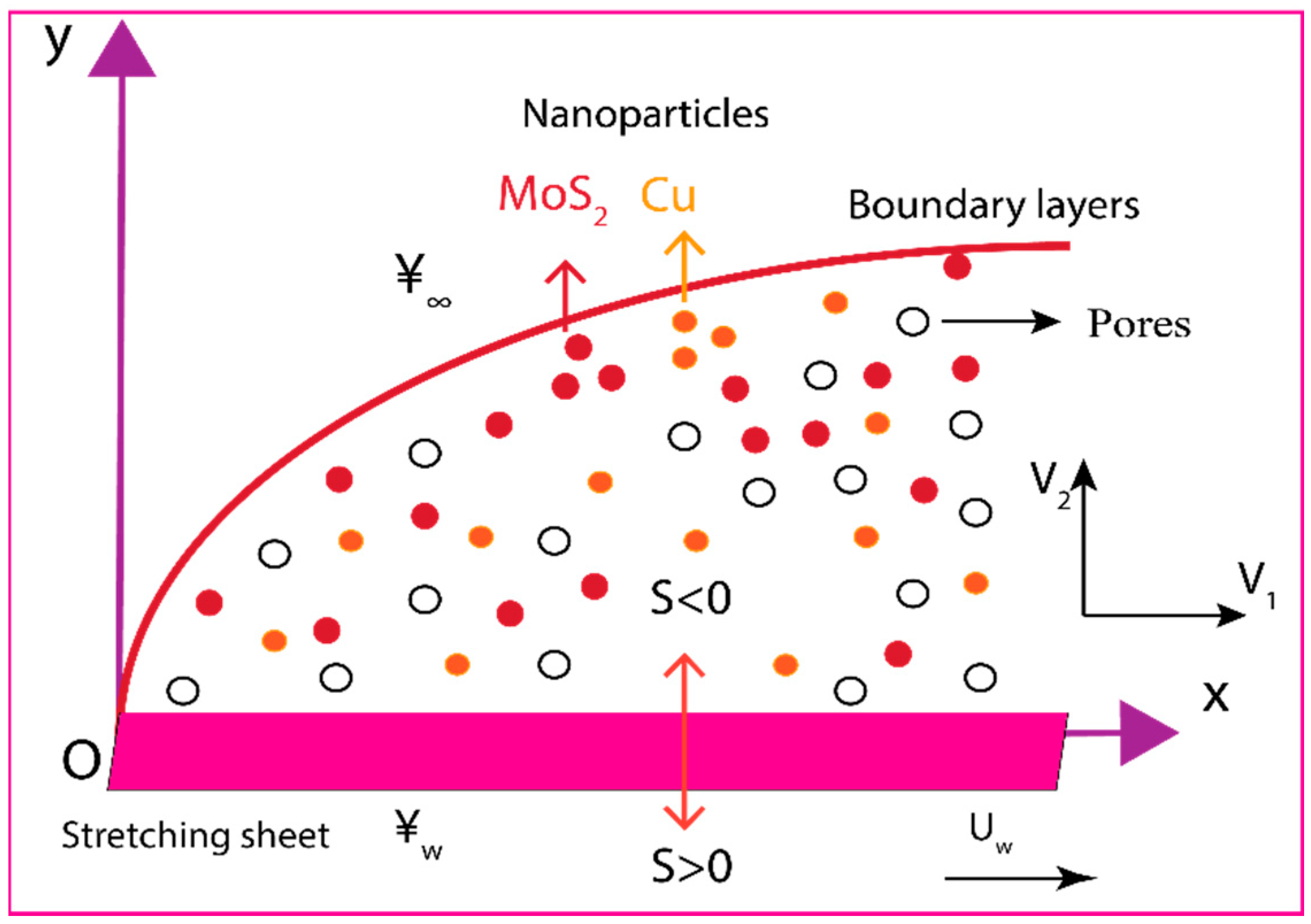
2. Mathematical Formulation
2.1. Model Equations
2.2. Thermophysical Features of the Oldroyd-B Nanofluid
2.3. Nanosolid-Particles and Base Fluid Attributes
2.4. Rosseland Approximations
3. The Solution to the Problem
3.1. Nusselt Number
3.2. Entropy Generation Analysis
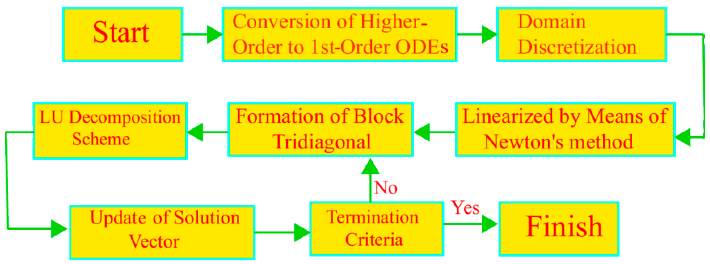
4. Numerical Implementation
Conversion of ODEs
5. Code Validation
6. Results and Discussion
7. Final Outcomes
- (a)
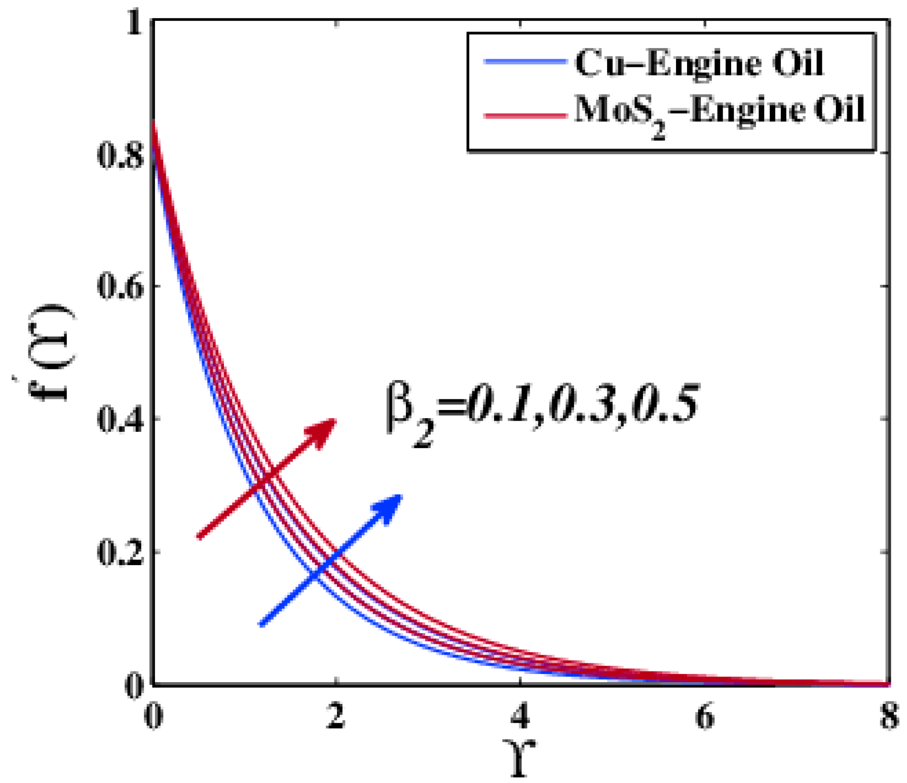
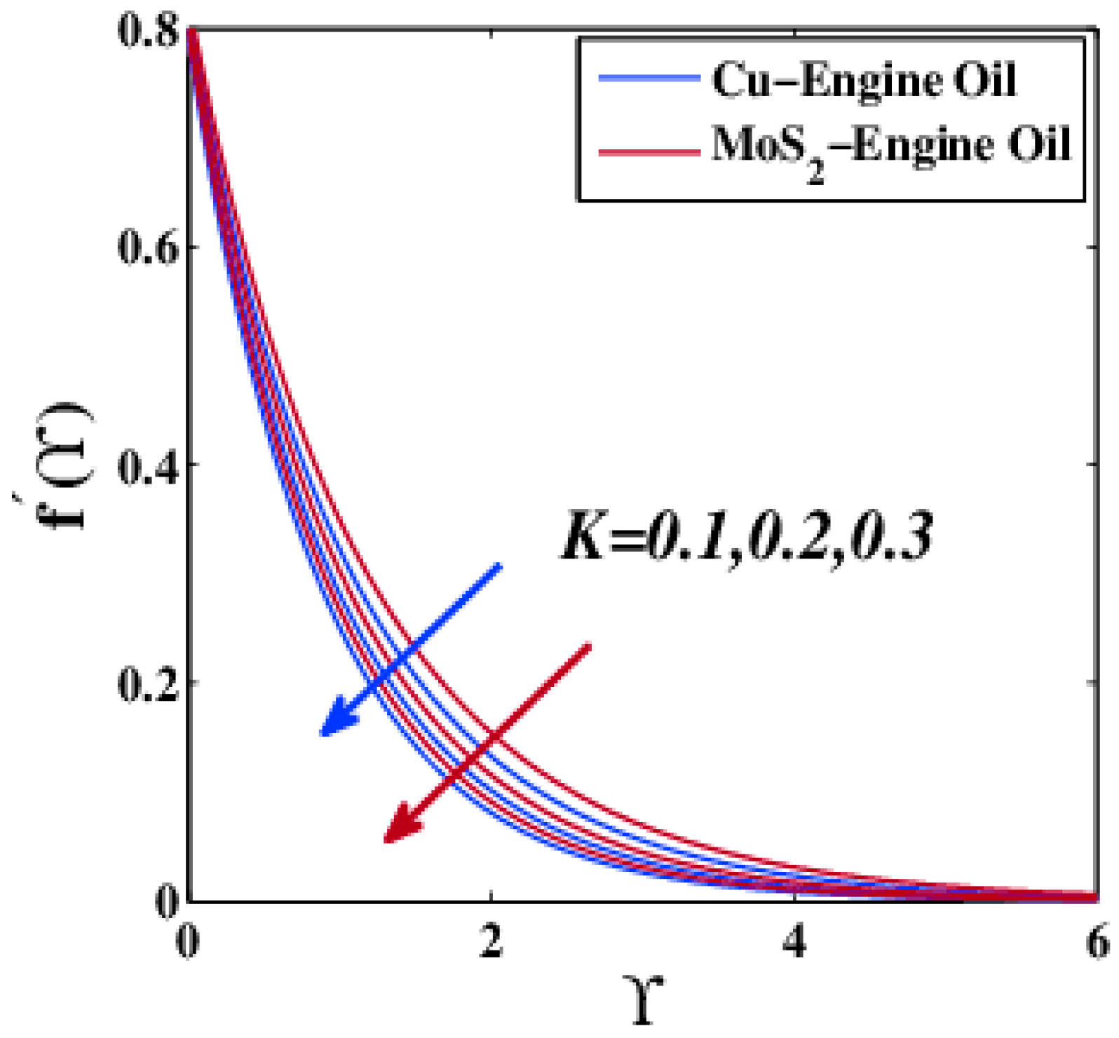
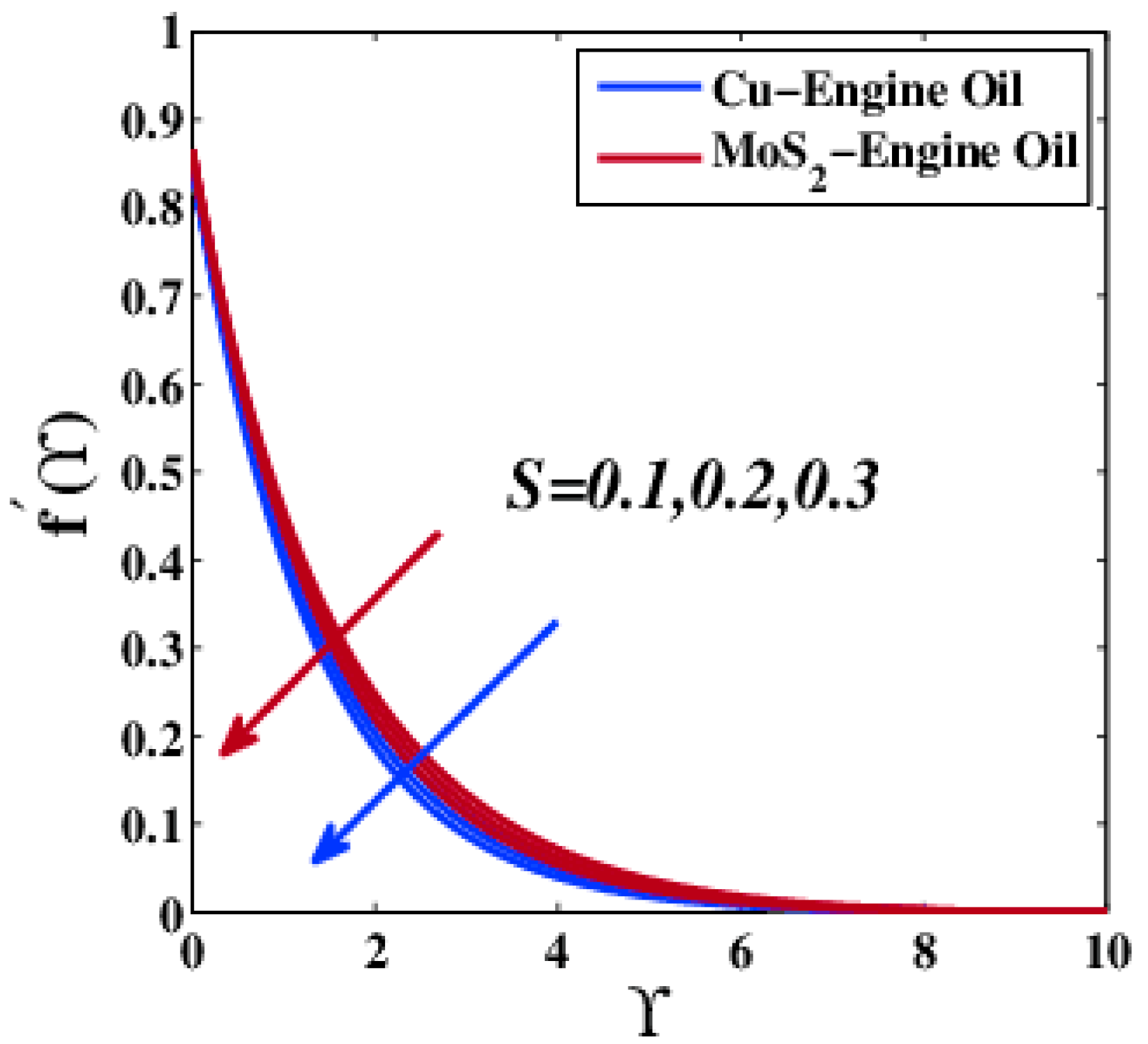
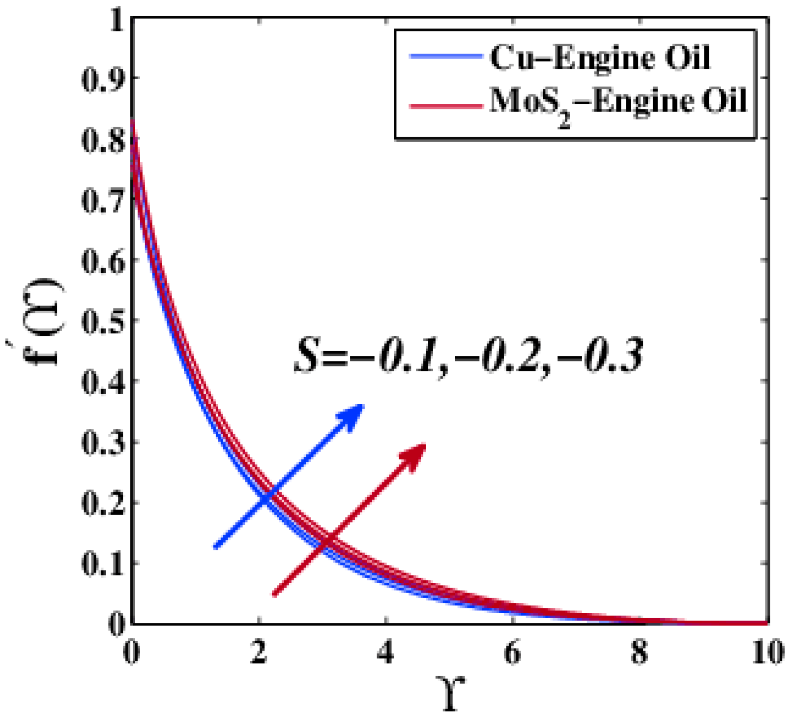
- An increase in velocity distribution was observed, under the influence of and . Otherwise, this profile decreased due to the increase of , , , and .
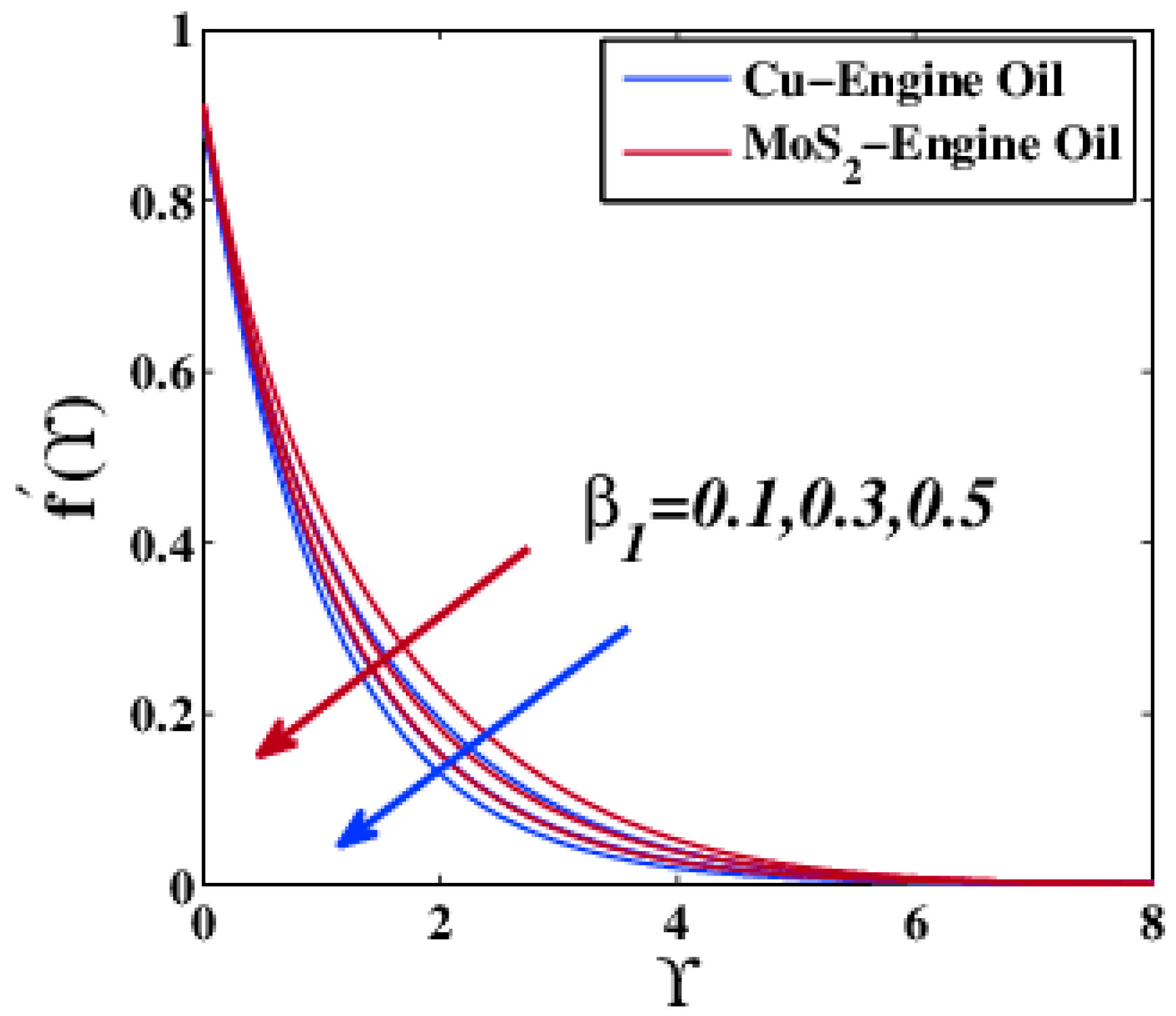
- (b)
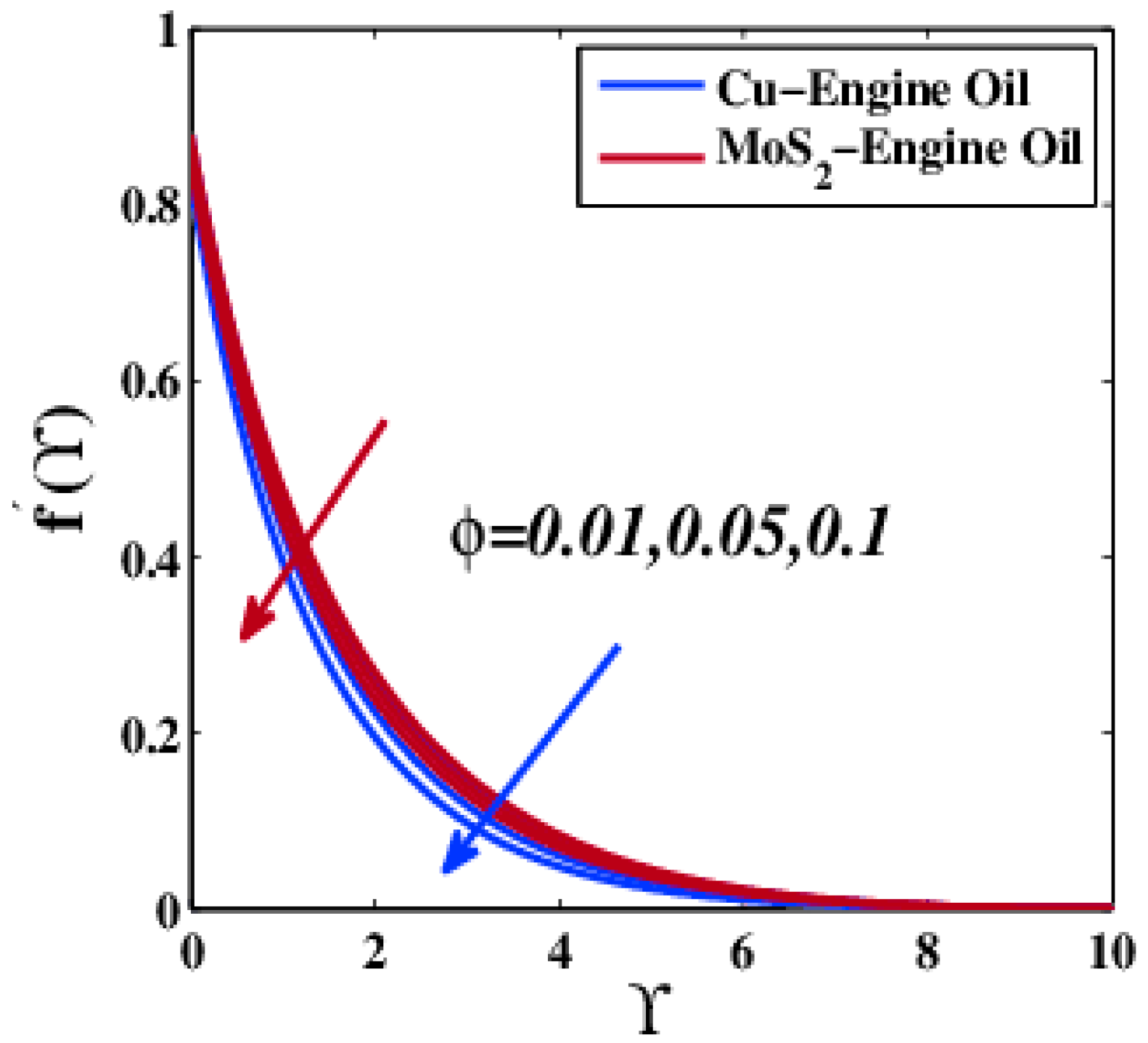
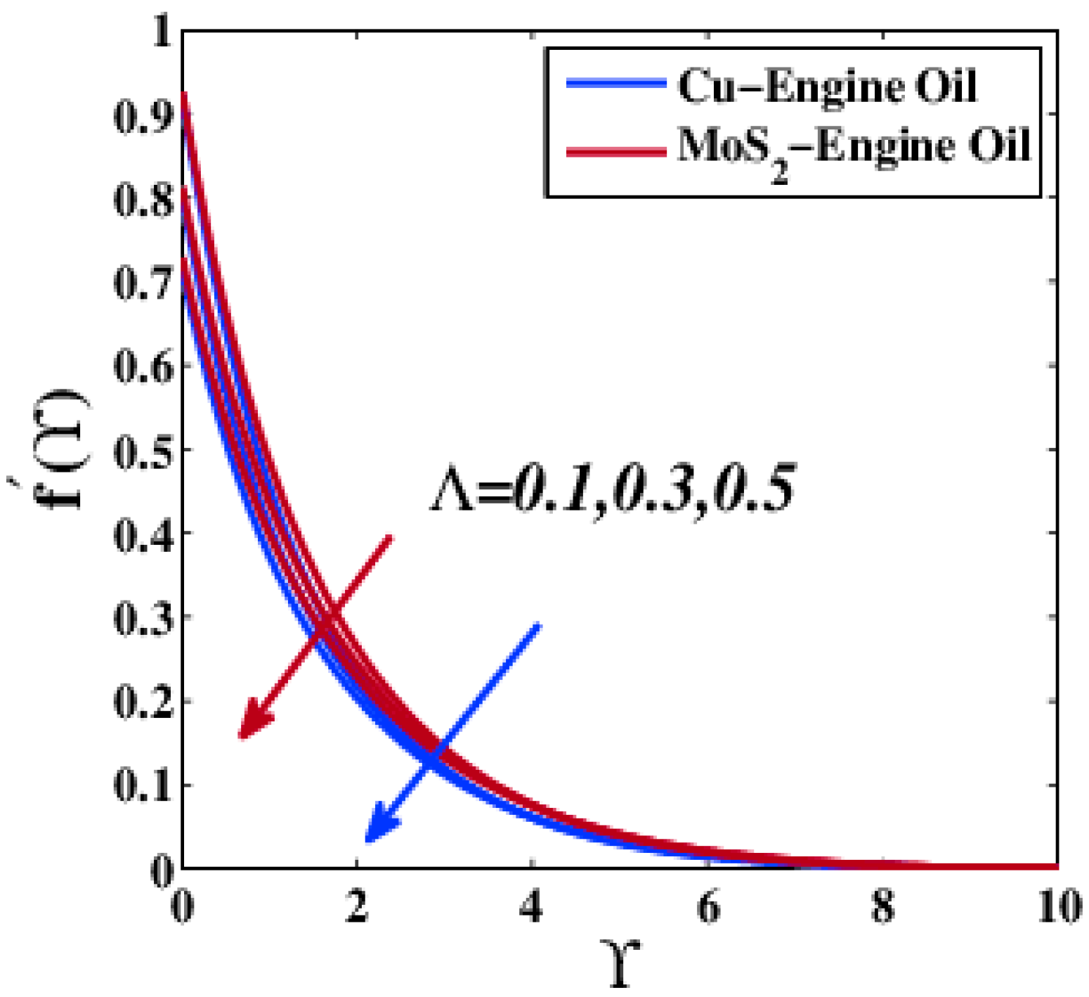
- The velocity of molybdenum disulfide engine oil (MoS2–EO) nanofluid was found to be higher than copper engine oil (Cu–EO) nanofluid. This comparison was depicted under the impact of the Deborah number, porous media parameter, nanoparticle volume fraction parameter, velocity slip parameter, suction, and injection.
- (c)
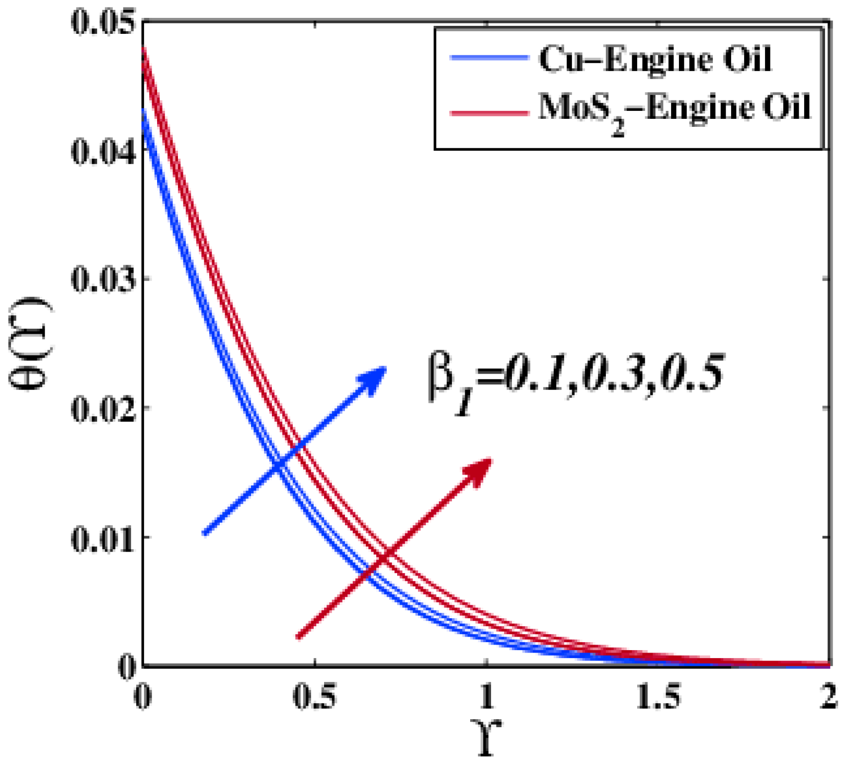
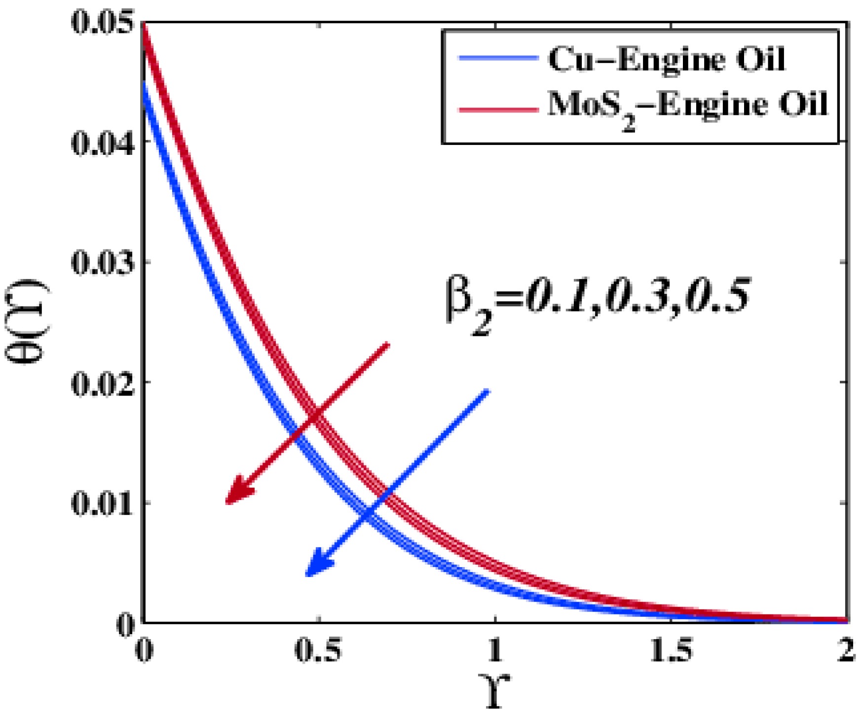
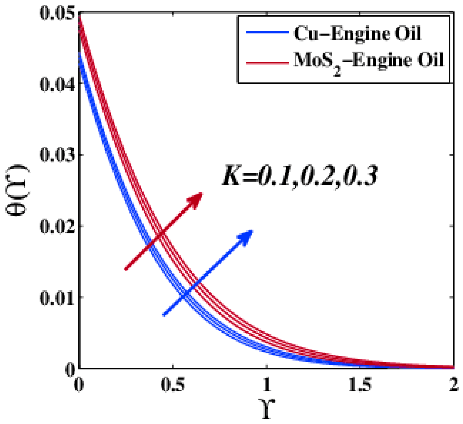
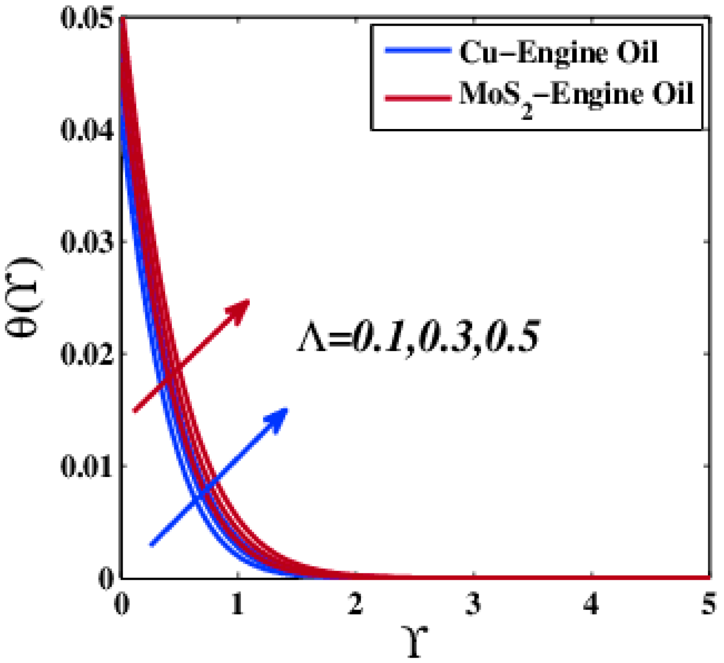
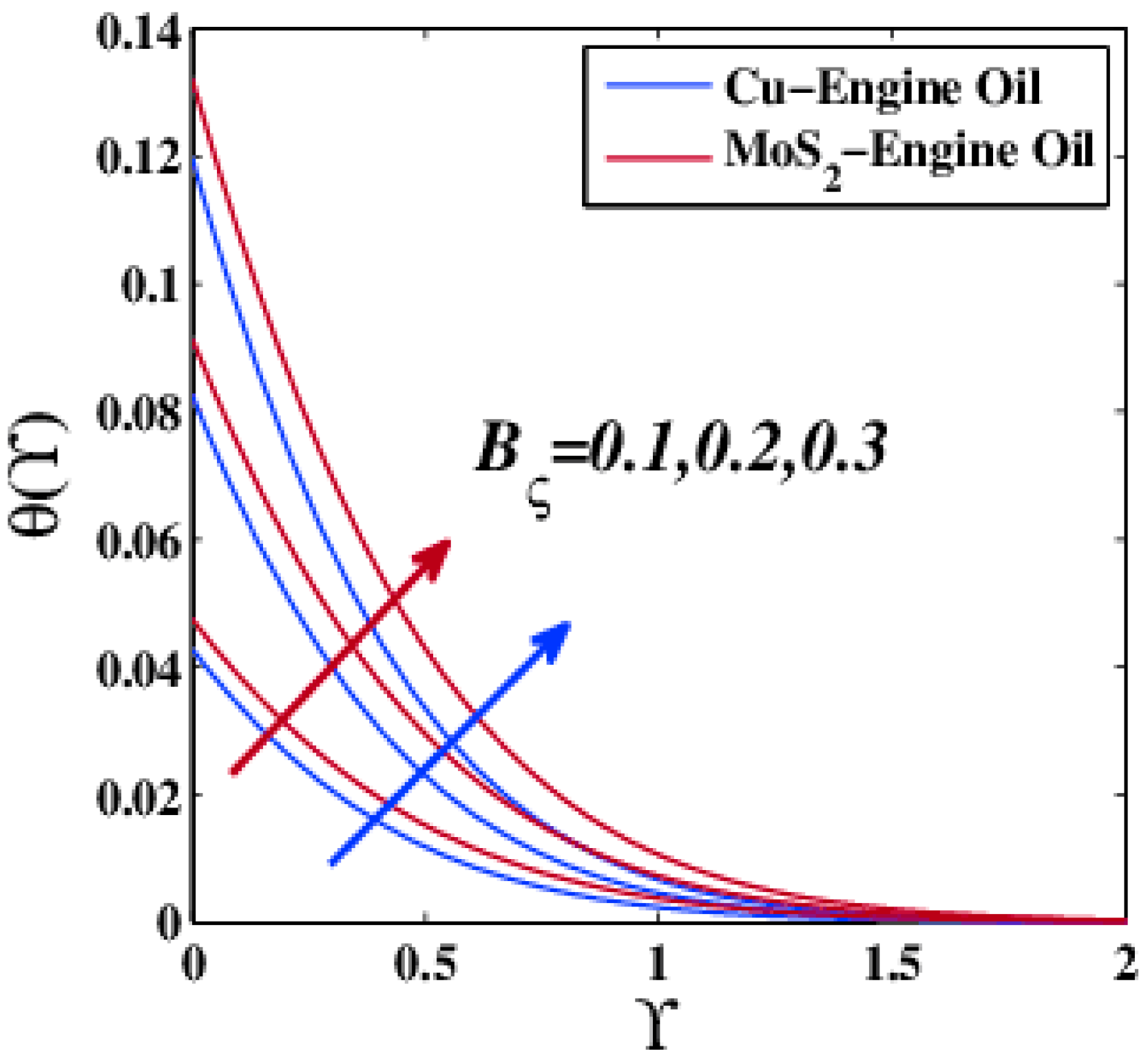
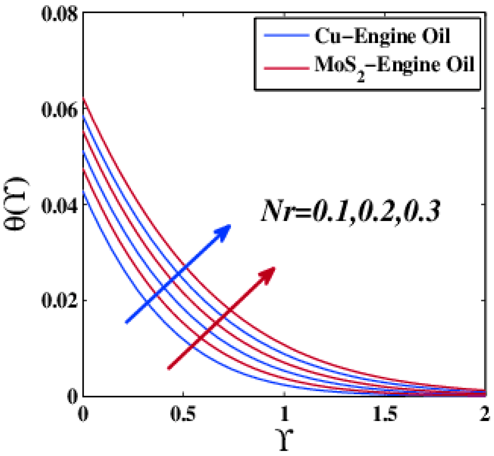
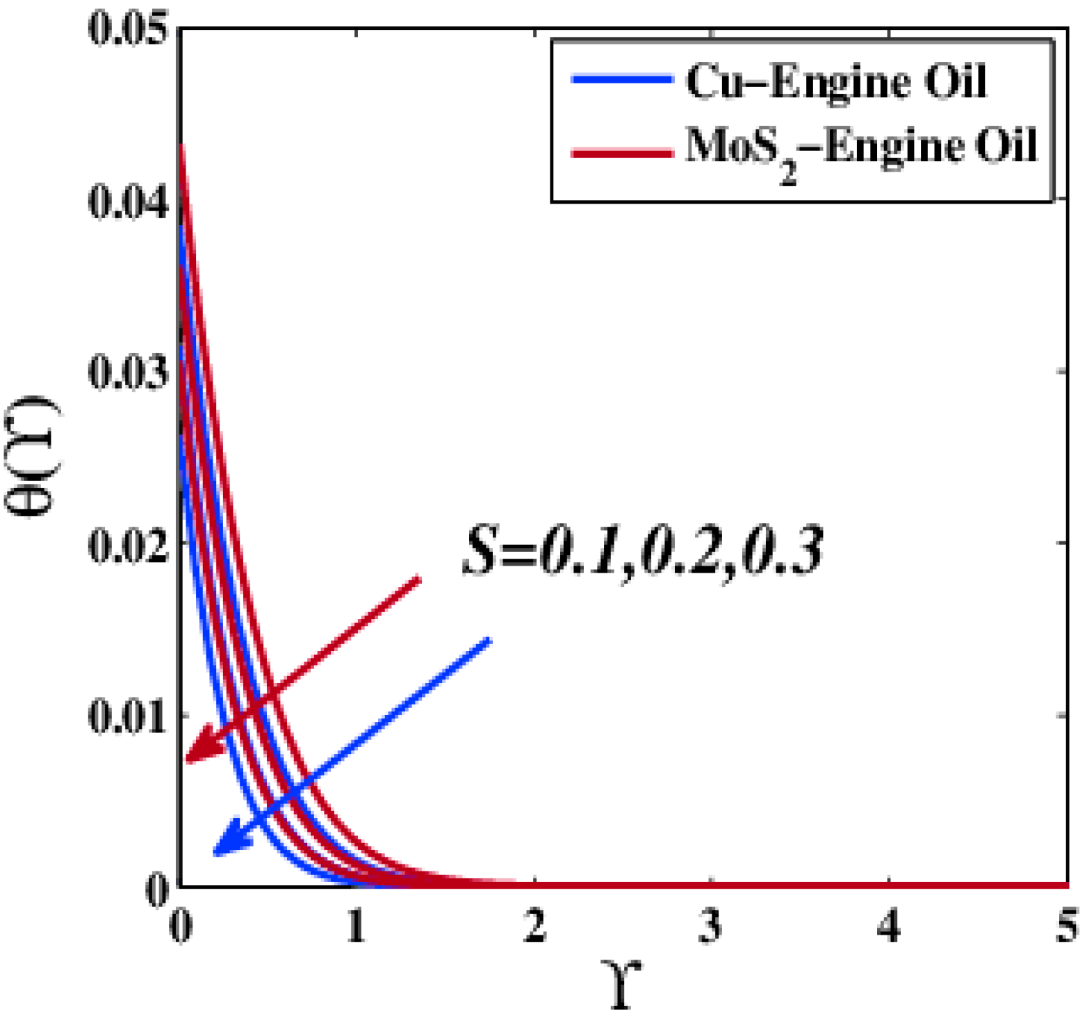
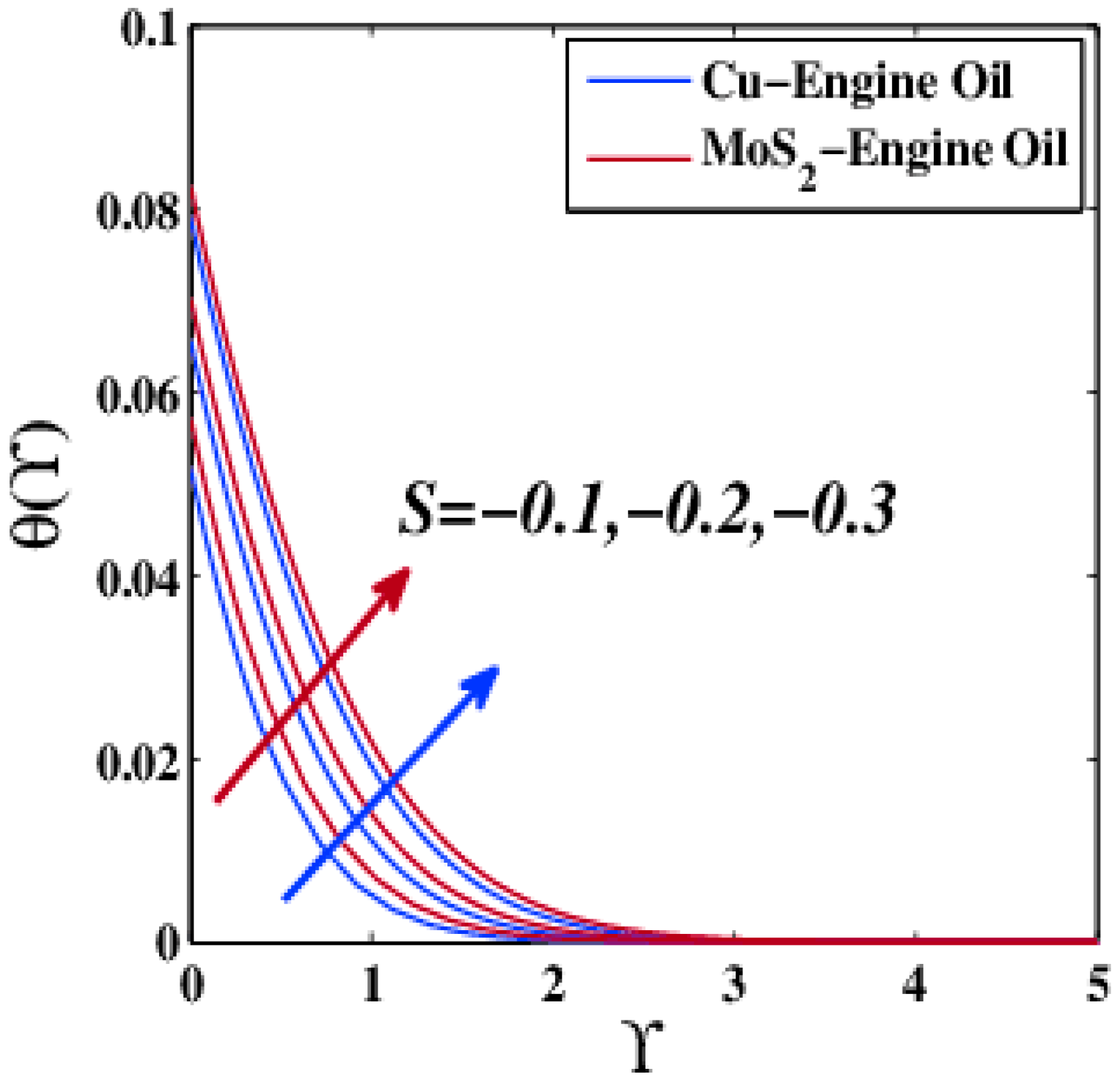
- The fluid temperature increased due to increasing values of , , , , , , , and . However, the same profile decreased due to and .
- (d)
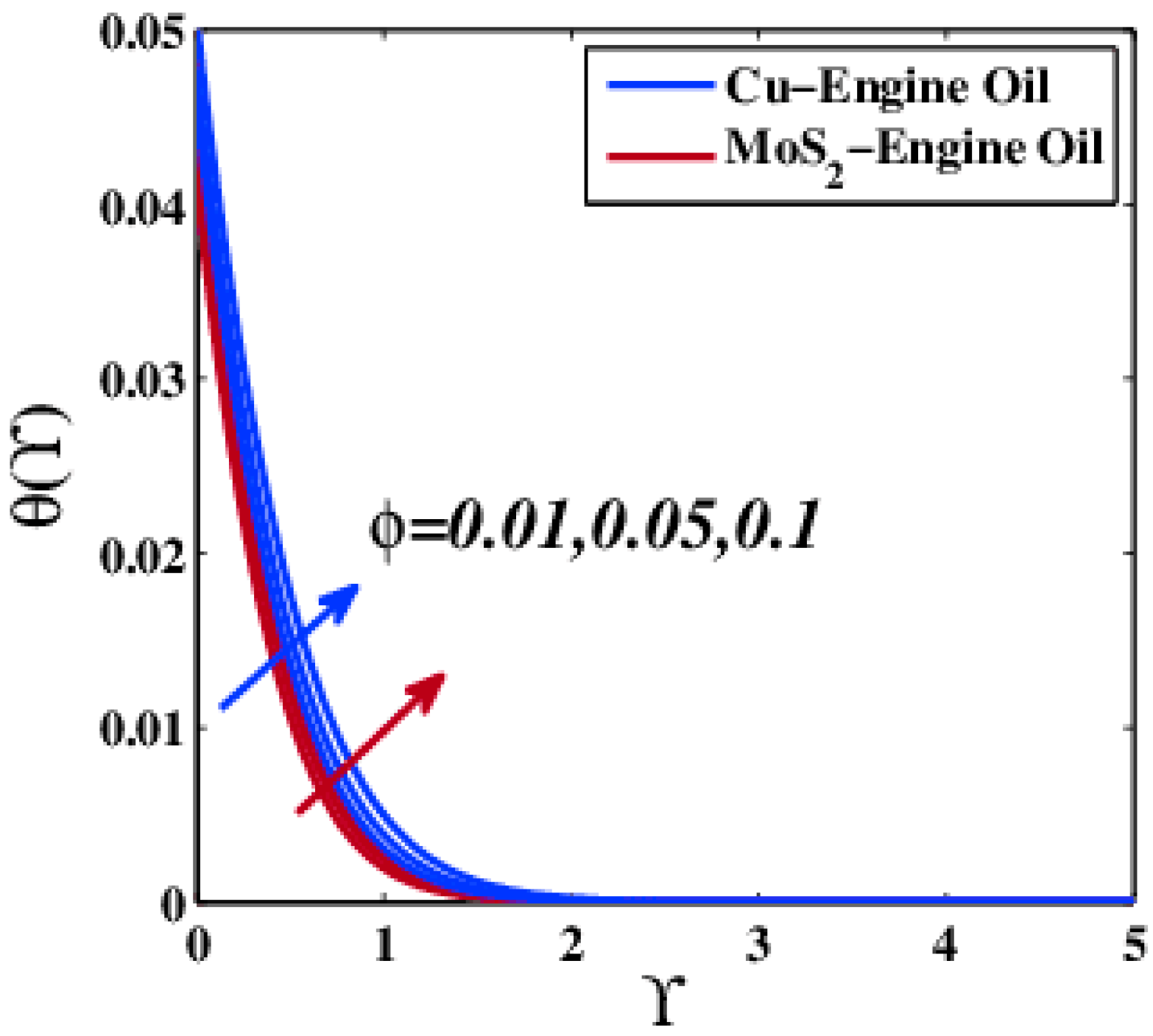
- Temperature profiles showed that the graphs for MoS2–EO were above those for the Cu–EO nanofluid. These two lines can be observed when varying controlling parameters such as the Deborah number, porous media parameter, velocity slip parameter, Biot number, variable thermal conductivity, radiation parameter, suction, and injection. However, the temperature measured for the Cu–EO nanofluid was greater than for MoS2–EO, for various values of the nanoparticle volume fraction parameter.
- (e)
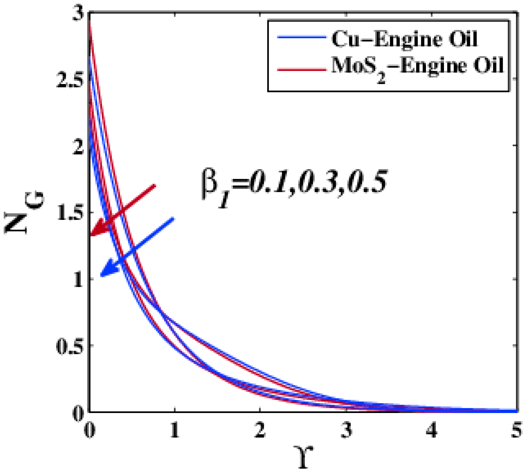
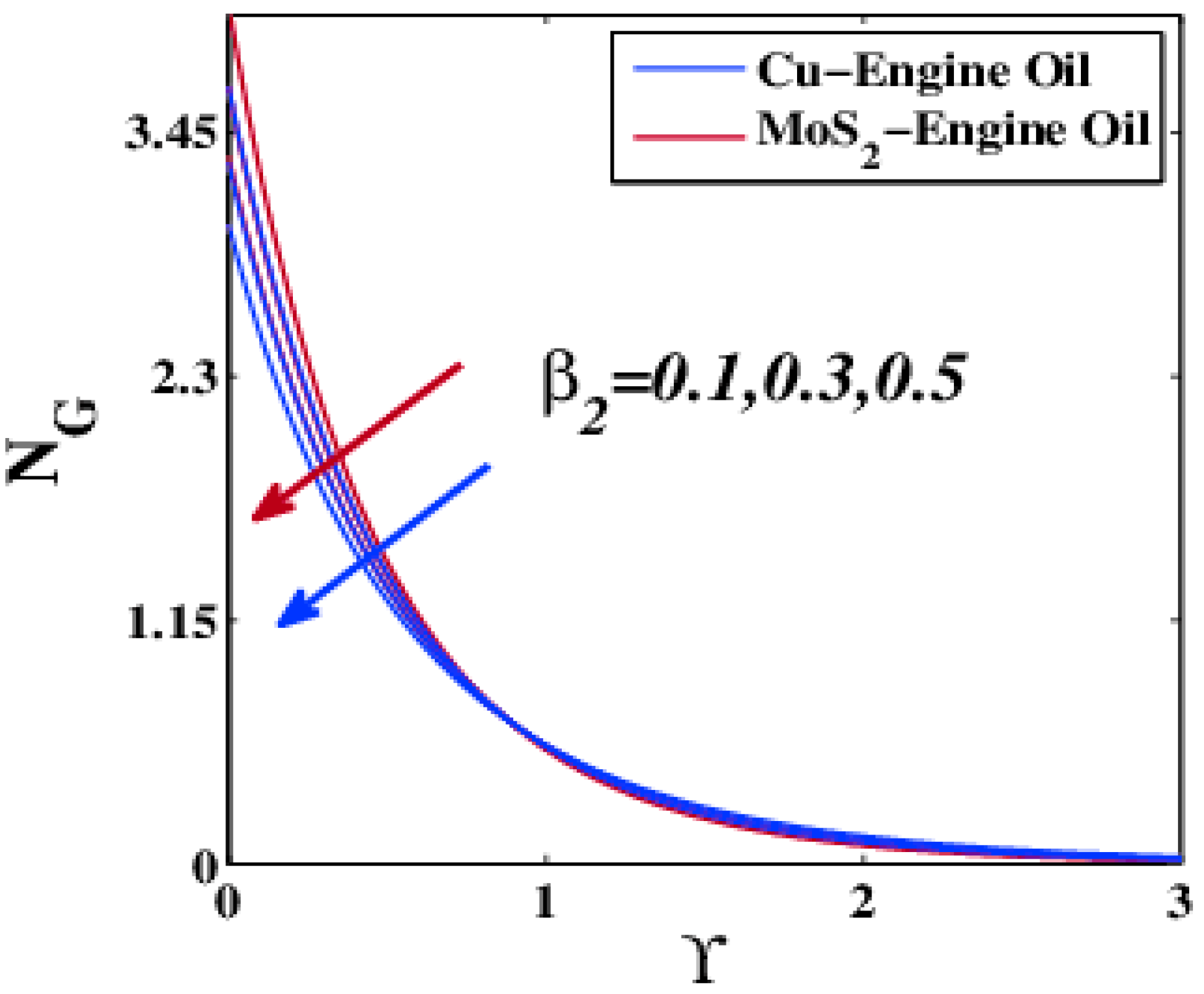
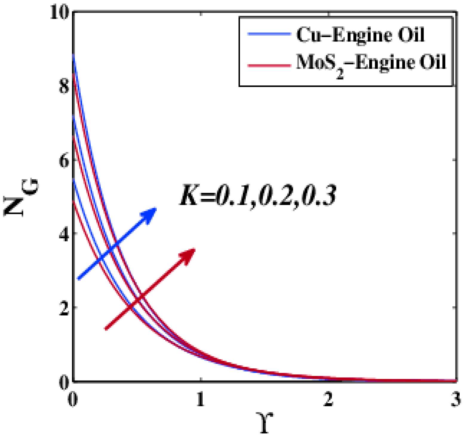
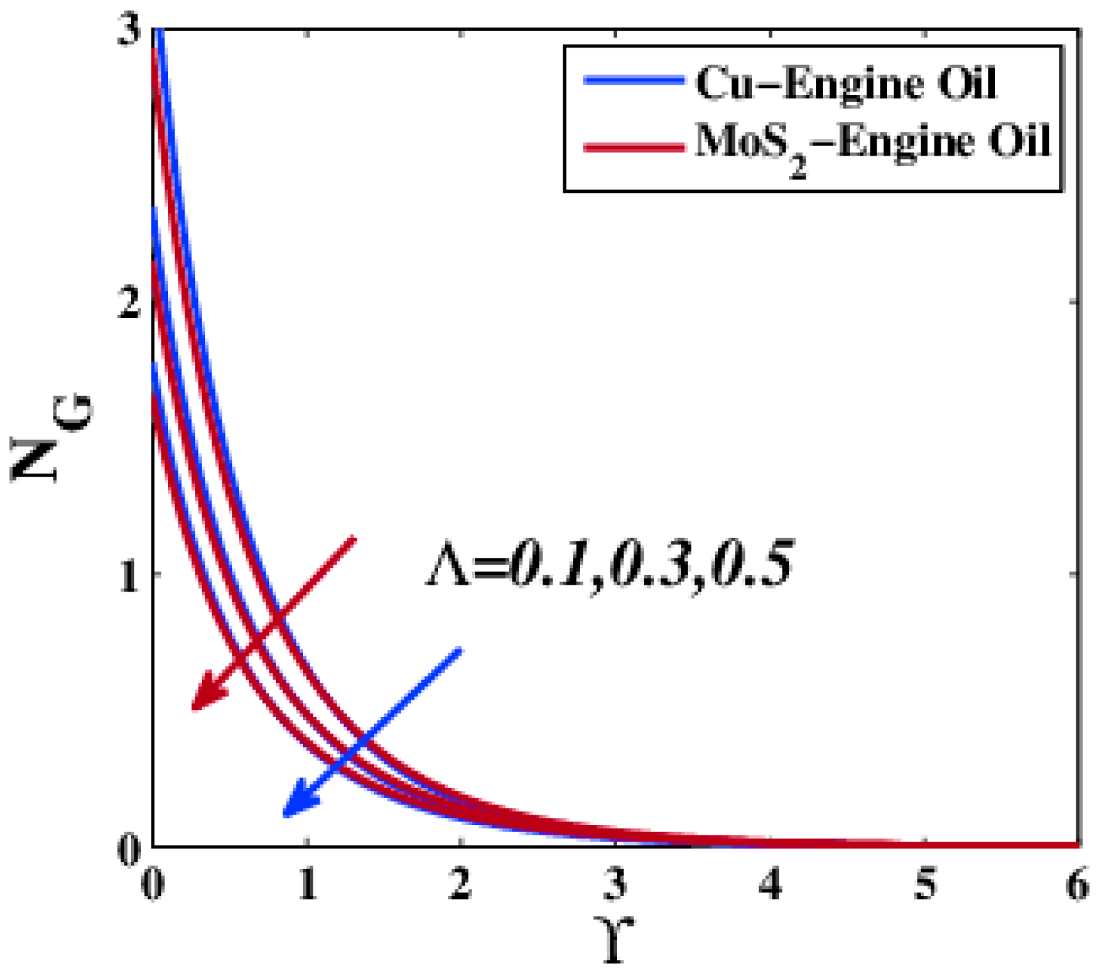
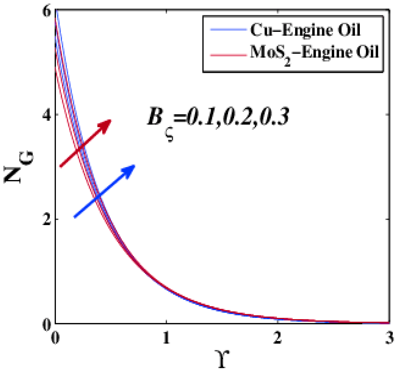
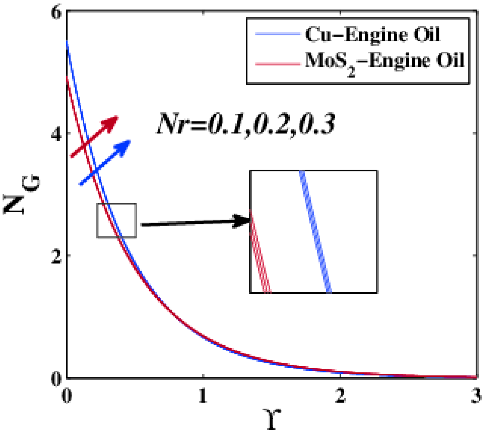
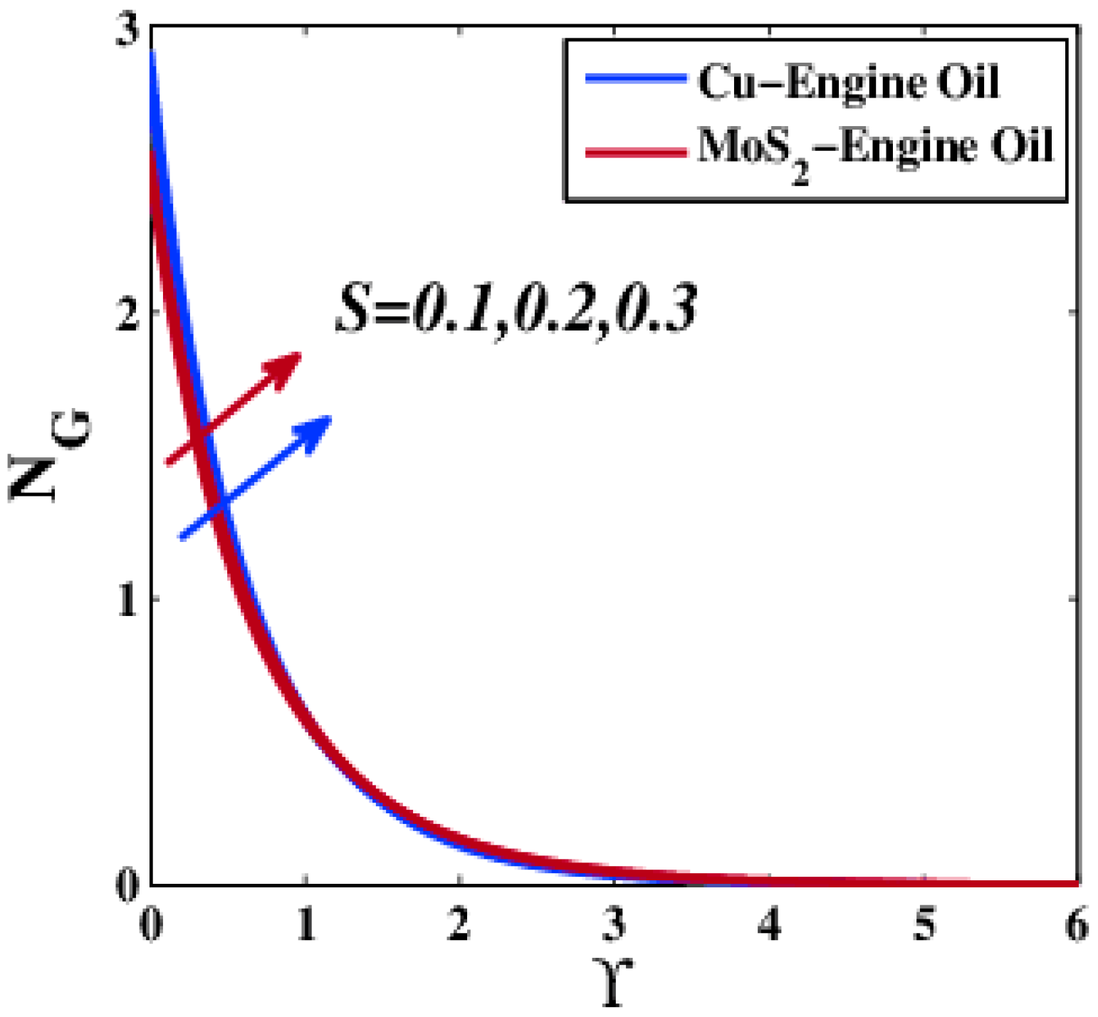
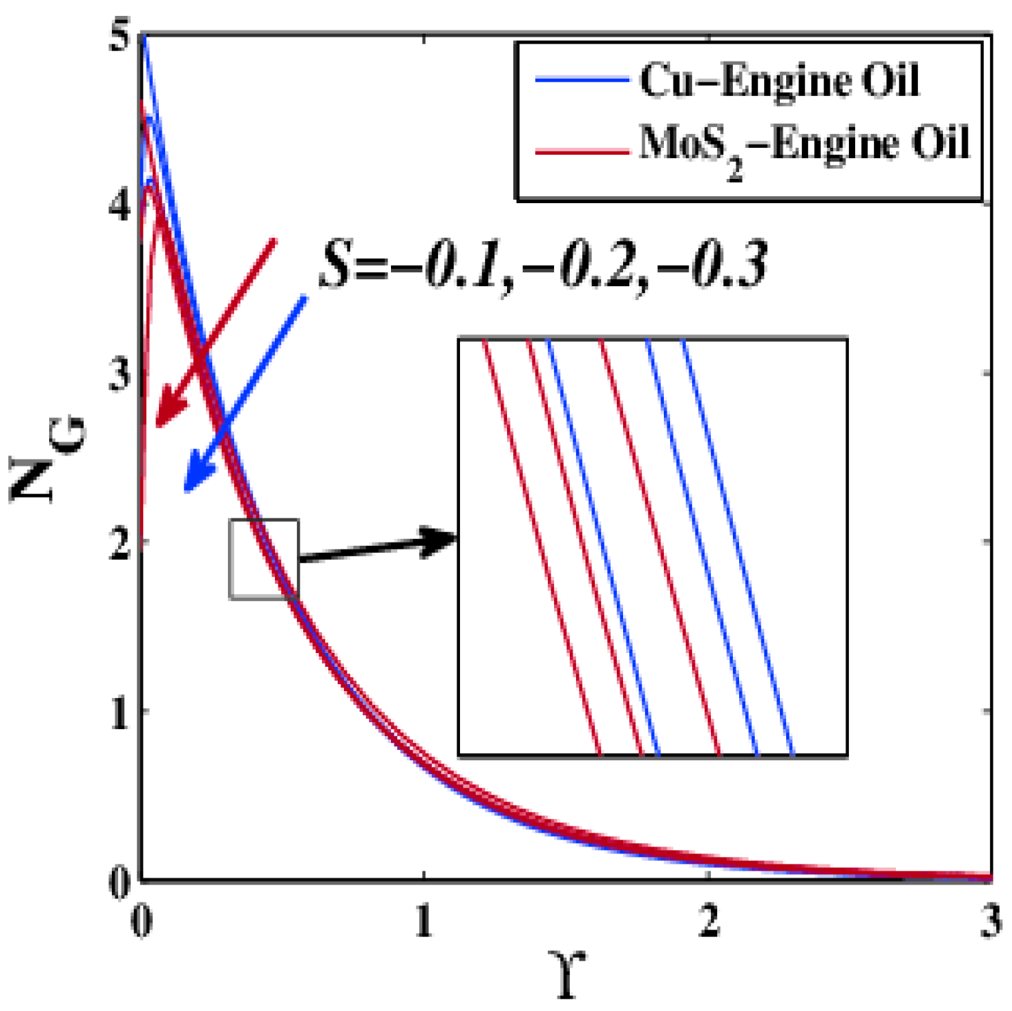
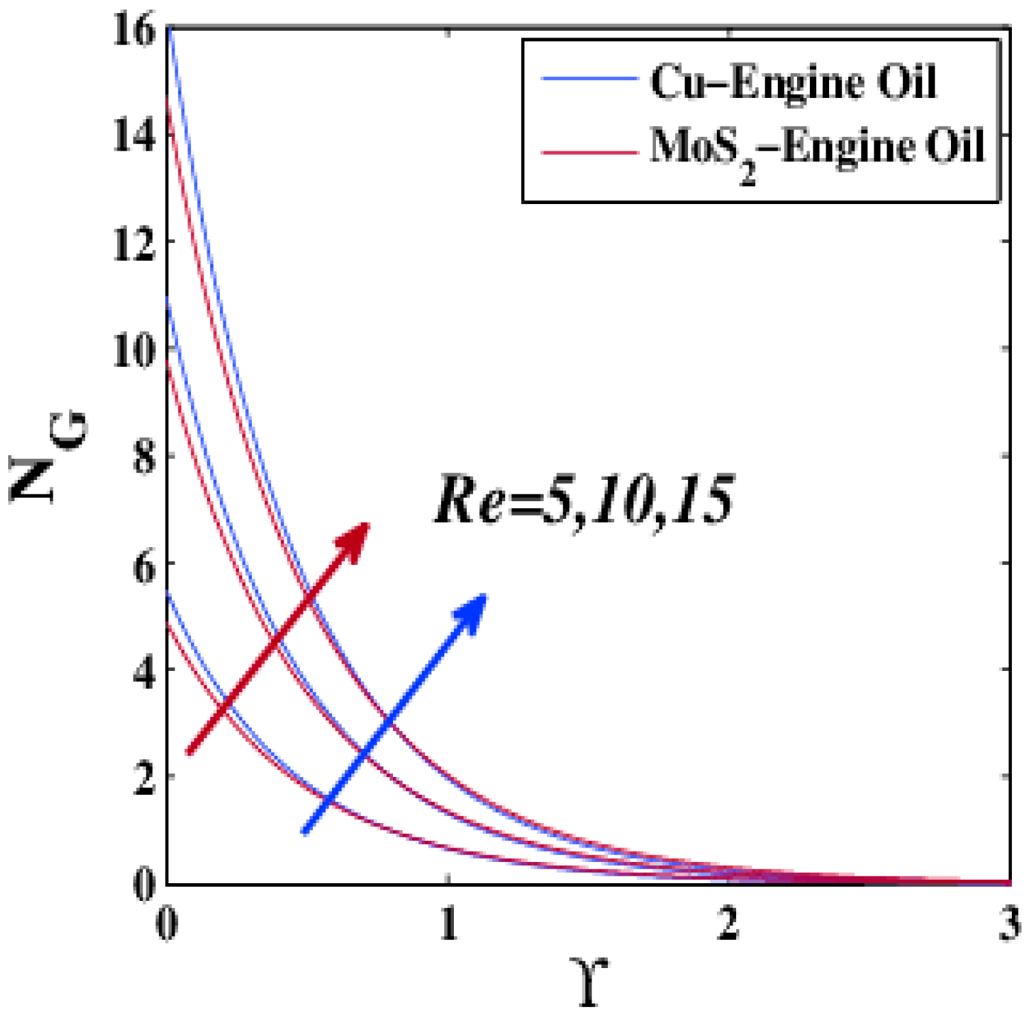
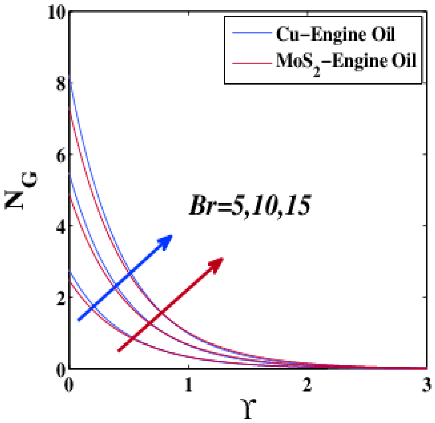
- The roles of Deborah number ( and ), velocity slip parameter, and injection parameter were to lessen the values of entropy generation. At the same time, this profile was enhanced when the following parameters increased: porous media parameter, volume friction parameter, Biot number, radiation parameter, suction parameter, Reynolds number, and Brinkman number.
- (f)
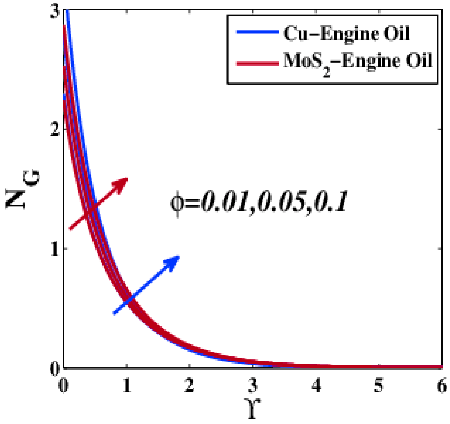
- At the small thickness boundary layer, the entropy generation of MoS2–EO was higher than that of Cu–EO when this profile was affected by Deborah number. Moreover, Cu–EO entropy generation was greatest for increasing series of porous media parameter, nanoparticle volume fraction parameter, velocity slip parameter, Biot number, radiation parameter, suction, injection, Reynolds number, and Brinkman number.
- (g)
- The local Nusselt number was an ascending function of , and . Moreover, the local Nusselt number was a decreasing function of . The effects of and are valid for both Cu–EO and MoS2–EO. However, the effect of on the local Nusselt number was described as follows: (i) decrease for Cu–EO; (ii) increase for MoS2–EO.
8. Future Direction
Author Contributions
Funding
Institutional Review Board Statement
Informed Consent Statement
Data Availability Statement
Conflicts of Interest
Nomenclatures
| initial stretching rate | Greek Symbols | ||
| Biot number | fluid temperature (K) | ||
| Brinkman number | fluid temperature of the surface (K) | ||
| skin friction coefficient | ambient temperature (K) | ||
| specific heat | volume fraction of the nanoparticles | ||
| dimensional entropy | density | ||
| Heat transfer coefficient | Stefan─Boltzmann constant | ||
| thermal conductivity | stream function | ||
| porous medium | independent similarity variable | ||
| absorption coefficient | dimensionless temperature | ||
| variable thermal conductivity | velocity slip | ||
| radiation parameter | dynamic viscosity () | ||
| dimensionless entropy generation | kinematic viscosity () | ||
| local Nusselt number | thermal diffusivity | ||
| Prandtl number | Deborah number-I | ||
| radiative heat flux | Deborah number-II | ||
| wall heat flux | dimensionless temperature gradient | ||
| Reynolds number | Subscripts | ||
| suction/injection parameter | base fluid | ||
| velocity component | particles | ||
| stretching velocity | nanofluid | ||
| vertical velocity | |||
| dimensional space coordinates | |||
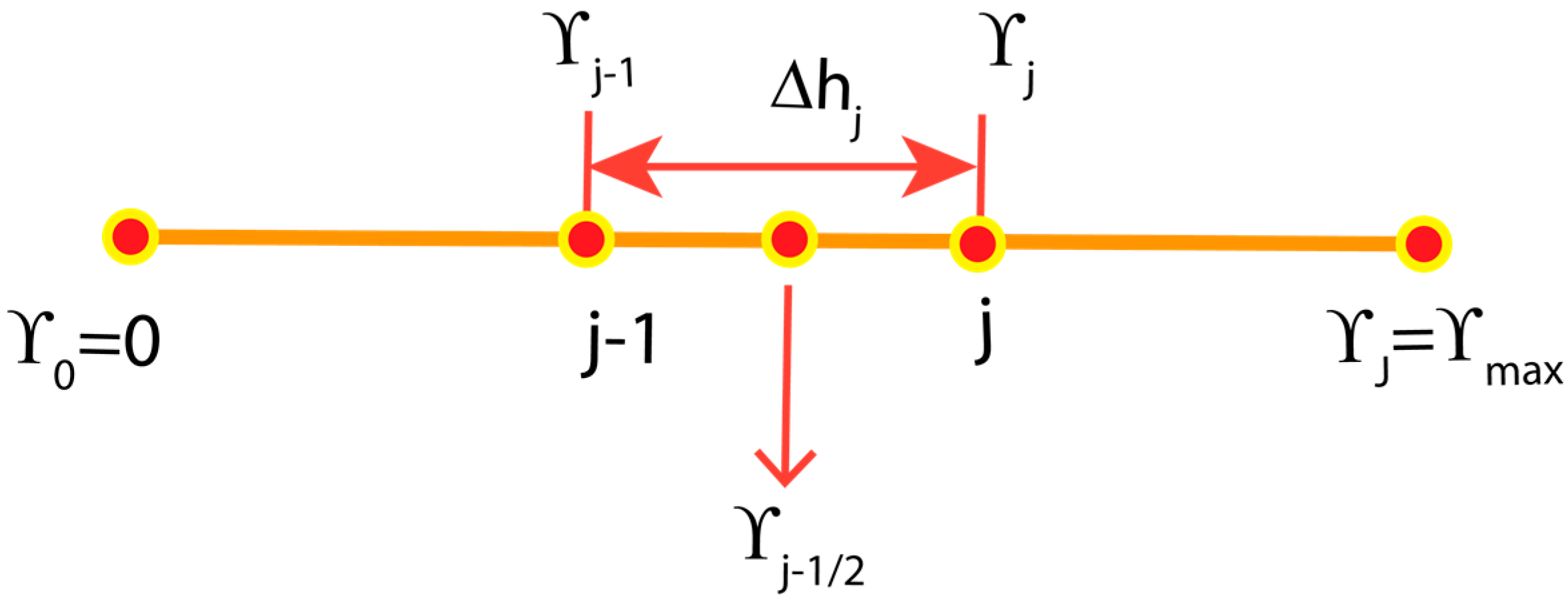
Appendix A. In This Part, We Give the Details of the Numerical Procedure for the Keller-Box Method
Appendix A.1. Difference Equations
Appendix A.2. Newton Linearization
Appendix A.3. Block Tridiagonal Structure
References
- Choi, S. Enhancing thermal conductivity of fluids with nanoparticles, developments, and applications of non-Newtonian flows. In Proceedings of the ASME International Mechanical Engineering Congress and Exposition, American Society of Mechanical Engineering, San Francisco, CA, USA, 12–17 November 1995; Volume 231, pp. 99–106. [Google Scholar]
- Kumar, N.; Hirschey, J.; LaClair, T.J.; Gluesenkamp, K.R.; Graham, S. Review of stability and thermal conductivity enhancements for salt hydrates. J. Energy Storage 2019, 24, 100794. [Google Scholar] [CrossRef]
- Abo-Elkhair, R.E.; Bhatti, M.M.; Mekheimer, K.S. Magnetic force effects on peristaltic transport of hybrid bio-nanofluid (AuCu nanoparticles) with moderate Reynolds number: An expanding horizon. Int. Commun. Heat Mass Transf. 2021, 123, 105228. [Google Scholar] [CrossRef]
- Mandhare, H.; Barai, D.P.; Bhanvase, B.A.; Saharan, V.K. Preparation and thermal conductivity investigation of reduced graphene oxide-ZnO nanocomposite-based nanofluid synthesised by ultrasound-assisted method. Mater. Res. Innov. 2020, 24, 433–441. [Google Scholar] [CrossRef]
- Ma, B.; Shin, D.; Banerjee, D. Synthesis and characterization of molten salt nanofluids for thermal energy storage application in concentrated solar power plants—Mechanistic understanding of specific heat capacity enhancement. Nanomaterials 2020, 10, 2266. [Google Scholar] [CrossRef] [PubMed]
- Ma, B.; Shin, D.; Banerjee, D. One-step synthesis of molten salt nanofluid for thermal energy storage application–a comprehensive analysis on thermophysical property, corrosion behavior, and economic benefit. J. Energy Storage 2021, 35, 102278. [Google Scholar] [CrossRef]
- Hady, F.M.; Ibrahim, F.S.; Abdel-Gaied, S.M.; Eid, M.R. Radiation effect on viscous flow of a nanofluid and heat transfer over a nonlinearly stretching sheet. Nanoscale Res. Lett. 2012, 7, 229. [Google Scholar] [CrossRef] [Green Version]
- Pinem, M.P.; Wardhono, E.Y.; Nadaud, F.; Clausse, D.; Saleh, K.; Guénin, E. Nanofluid to nanocomposite film: Chitosan and cellulose-based edible packaging. Nanomaterials 2020, 10, 660. [Google Scholar] [CrossRef] [Green Version]
- Chen, H.; Chen, Z.; Yang, H.; Wang, J.; Zhao, H. Lowest liquid phase saturation point temperature–phase separation–viscosity model for the optimal formulation of mixed fluoride salt. Sol. Energy Mater. Sol. Cells 2021, 227, 111107. [Google Scholar] [CrossRef]
- Rakkappan, S.R.; Sivan, S.; Ahmed, S.N.; Naarendharan, M.; Sudhir, P.S. Preparation, characterisation and energy storage performance study on 1-Decanol-expanded graphite composite PCM for air-conditioning cold storage system. Int. J. Refrig. 2021, 123, 91–101. [Google Scholar] [CrossRef]
- Li, Y.-X.; Alqsair, U.F.; Ramesh, K.; Khan, S.U.; Khan, M.I. Nonlinear heat source/sink and activation energy assessment in double diffusion flow of micropolar (non-Newtonian) nanofluid with convective conditions. Arab. J. Sci. Eng. 2021, in press. [Google Scholar] [CrossRef]
- Ali, W.; Mahmood, S.; Chammam, W.; Ul-Haq, W.; Khan, W.A.; Abbas, S.Z. Mathematical modeling and chemical conduct considering non-Newtonian nanofluid by utilizing heat flux features. Soft Comput. 2020, 24, 11829–11839. [Google Scholar] [CrossRef]
- Abbas, S.Z.; Farooq, S.; Chu, Y.M.; Chammam, W.; Khan, W.A.; Riahi, A.; Rebei, H.A.; Zaway, M. Numerical study of nanofluid transport subjected to the collective approach of generalized slip condition and radiative phenomenon. Arab. J. Sci. Eng. 2021, 46, 6049–6059. [Google Scholar] [CrossRef]
- Irfan, M.; Khan, M.; Khan, W.; Alghamdi, M.; Ullah, M.Z. Influence of thermal-solutal stratifications and thermal aspects of non-linear radiation in stagnation point Oldroyd-B nanofluid flow. Int. Commun. Heat Mass Transf. 2020, 116, 104636. [Google Scholar] [CrossRef]
- Anwar, T.; Kumam, P.; Baleanu, D.; Khan, I.; Thounthong, P. Radiative heat transfer enhancement in MHD porous channel flow of an Oldroyd-B fluid under generalized boundary conditions. Phys. Scr. 2020, 95, 115211. [Google Scholar] [CrossRef]
- Ramzan, M.; Howari, F.; Chung, J.D.; Kadry, S.; Chu, Y.-M. Irreversibility minimization analysis of ferromagnetic Oldroyd-B nanofluid flow under the influence of a magnetic dipole. Sci. Rep. 2021, 11, 4810. [Google Scholar] [CrossRef]
- Abbas, S.; Khan, W.; Waqas, M.; Irfan, M.; Asghar, Z. Exploring the features for flow of Oldroyd-B liquid film subjected to rotating disk with homogeneous/heterogeneous processes. Comput. Methods Programs Biomed. 2020, 189, 105323. [Google Scholar] [CrossRef]
- Waqas, H.; Imran, M.; Muhammad, T.; Sait, S.M.; Ellahi, R. Numerical investigation on bioconvection flow of Oldroyd-B nanofluid with nonlinear thermal radiation and motile microorganisms over rotating disk. J. Therm. Anal. Calorim. 2020, 145, 523–539. [Google Scholar] [CrossRef]
- Tulu, A.; Ibrahim, W. Effects of second-order slip flow and variable viscosity on natural convection flow of CNTs–Fe3O4/Water hybrid nanofluids due to stretching surface. Math. Probl. Eng. 2021, 2021, 84097194. [Google Scholar] [CrossRef]
- Eid, M.R.; Nafe, M.A. Thermal conductivity variation and heat generation effects on magneto-hybrid nanofluid flow in a porous medium with slip condition. Waves Random Complex Media 2020, 1–25. [Google Scholar] [CrossRef]
- Li, Q.; Li, C.; Du, Z.; Jiang, F.; Ding, Y. A review of performance investigation and enhancement of shell and tube thermal energy storage device containing molten salt based phase change materials for medium and high temperature applications. Appl. Energy 2019, 255, 113806. [Google Scholar] [CrossRef]
- Hussien, A.A.; Abdullah, M.Z.; Yusop, N.M.; Al-Kouz, W.; Mahmoudi, E.; Mehrali, M. Heat transfer and entropy generation abilities of MWCNTs/GNPs hybrid nanofluids in microtubes. Entropy 2019, 21, 480. [Google Scholar] [CrossRef] [PubMed] [Green Version]
- Ahmad, S.; Nadeem, S.; Ullah, N. Entropy generation and temperature-dependent viscosity in the study of SWCNT-MWCNT hybrid nanofluid. Appl. Nanosci. 2020, 10, 5107–5119. [Google Scholar] [CrossRef]
- Kumar, V.; Sarkar, J. Particle ratio optimization of Al2O3-MWCNT hybrid nanofluid in minichannel heat sink for best hydrothermal performance. Appl. Therm. Eng. 2020, 165, 114546. [Google Scholar] [CrossRef]
- Kumar, V.; Sarkar, J. Experimental hydrothermal behavior of hybrid nanofluid for various particle ratios and comparison with other fluids in minichannel heat sink. Int. Commun. Heat Mass Transf. 2019, 110, 104397. [Google Scholar] [CrossRef]
- Ma, H.; Duan, Z.; Su, L.; Ning, X.; Bai, J.; Lv, X. Fluid flow and entropy generation analysis of Al2O3-water nanofluid in microchannel plate fin heat sinks. Entropy 2019, 21, 739. [Google Scholar] [CrossRef] [PubMed] [Green Version]
- Abu-Libdeh, N.; Redouane, F.; Aissa, A.; Mebarek-Oudina, F.; Almuhtady, A.; Jamshed, W.; Al-Kouz, W. Hydrothermal and entropy investigation of Ag/MgO/H2O hybrid nanofluid natural convection in a novel shape of porous cavity. Appl. Sci. 2021, 11, 1722. [Google Scholar] [CrossRef]
- Almuhtady, A.; Alhazmi, M.; Al-Kouz, W.; Raizah, Z.; Ahmed, S. Entropy generation and MHD convection within an inclined trapezoidal heated by triangular fin and filled by a variable porous media. Appl. Sci. 2021, 11, 1951. [Google Scholar] [CrossRef]
- Tiwari, R.K.; Das, M.K. Heat transfer augmentation in a two-sided lid-driven differentially heated square cavity utilizing nanofluids. Int. J. Heat Mass Transf. 2007, 50, 2002–2018. [Google Scholar] [CrossRef]
- Mabood, F.; Bognár, G.; Shafiq, A. Impact of heat generation/absorption of magnetohydrodynamics Oldroyd-B fluid impinging on an inclined stretching sheet with radiation. Sci. Rep. 2020, 10, 17688. [Google Scholar] [CrossRef]
- Aziz, A.; Jamshed, W.; Aziz, T.; Bahaidarah, H.M.S.; Rehman, K.U. Entropy analysis of Powell–Eyring hybrid nanofluid including effect of linear thermal radiation and viscous dissipation. J. Therm. Anal. Calorim. 2020, 143, 1331–1343. [Google Scholar] [CrossRef]
- Jamshed, W.; Nisar, K.S.; Gowda, R.J.P.; Kumar, R.N.; Prasannakumara, B.C. Radiative heat transfer of second grade nanofluid flow past a porous flat surface: A single-phase mathematical model. Phys. Scr. 2021, 96, 064006. [Google Scholar] [CrossRef]
- Jamshed, W.; Aziz, A. A comparative entropy based analysis of Cu and Fe3O4/methanol Powell-Eyring nanofluid in solar thermal collectors subjected to thermal radiation, variable thermal conductivity and impact of different nanoparticles shape. Results Phys. 2018, 9, 195–205. [Google Scholar] [CrossRef]
- Arunachalam, M.; Rajappa, N.R. Forced convection in liquid metals with variable thermal conductivity and capacity. Acta Mech. 1978, 31, 25–31. [Google Scholar] [CrossRef]
- Mukhtar, T.; Jamshed, W.; Aziz, A.; Kouz, W.A. Computational investigation of heat transfer in a flow subjected to MHD of Maxwell nanofluid over a stretched flat sheet with thermal radiation. Numer. Methods Partial. Differ. Equ. 2020, in press. [Google Scholar] [CrossRef]
- Iqbal, Z.; Azhar, E.; Maraj, E.N. Performance of nano-powders SiO2 and SiC in the flow of engine oil over a rotating disk influenced by thermal jump conditions. Phys. A 2021, 565, 125570. [Google Scholar] [CrossRef]
- Brewster, M.Q. Thermal Radiative Transfer and Features; John Wiley and Sons: New York, NY, USA, 1992. [Google Scholar]
- Jamshed, W. Numerical investigation of MHD impact on Maxwell nanofluid. Int. Commun. Heat Mass Transf. 2021, 120, 104973. [Google Scholar] [CrossRef]
- Jamshed, W.; Nisar, K.S. Computational single phase comparative study of williamson nanofluid in parabolic trough solar collector via Keller box method. Int. J. Energy Res. 2021, 45, 10696–10718. [Google Scholar] [CrossRef]
- Jamshed, W.; Eid, M.R.; Nasir, N.A.A.M.; Nisar, K.S.; Aziz, A.; Shahzad, F.; Saleel, C.A.; Shukla, A. Thermal examination of renewable solar energy in parabolic trough solar collector utilizing Maxwell nanofluid: A noble case study. Case Stud. Therm. Eng. 2021, 27, 101258. [Google Scholar] [CrossRef]
- Jamshed, W.; Mishra, S.; Pattnaik, P.; Nisar, K.S.; Devi, S.S.U.; Prakash, M.; Shahzad, F.; Hussain, M.; Vijayakumar, V. Features of entropy optimization on viscous second grade nanofluid streamed with thermal radiation: A Tiwari and Das model. Case Stud. Therm. Eng. 2021, 27, 101291. [Google Scholar] [CrossRef]
- Jamshed, W.; Akgül, E.K.; Nisar, K.S. Keller box study for inclined magnetically driven Casson nanofluid over a stretching sheet: Single phase model. Phys. Scr. 2021, 96, 065201. [Google Scholar] [CrossRef]
- Jamshed, W.; Devi, S.U.; Nisar, K.S. Single phase based study of Ag-Cu/EO Williamson hybrid nanofluid flow over a stretching surface with shape factor. Phys. Scr. 2021, 96, 065202. [Google Scholar] [CrossRef]
- Jamshed, W.; Nisar, K.S.; Ibrahim, R.W.; Shahzad, F.; Eid, M.R. Thermal expansion optimization in solar aircraft using tangent hyperbolic hybrid nanofluid: A solar thermal application. J. Mater. Res. Technol. 2021, 14, 985–1006. [Google Scholar] [CrossRef]
- Jamshed, W.; Eid, M.R.; Nisar, K.S.; Nasir, N.A.A.M.; Edacherian, A.; Saleel, C.A.; Vijayakumar, V. A numerical frame work of magnetically driven Powell-Eyring nanofluid using single phase model. Sci. Rep. 2021, 11, 16500. [Google Scholar] [CrossRef]
- Jamshed, W. Thermal augmentation in solar aircraft using tangent hyperbolic hybrid nanofluid: A solar energy application. Energy Environ. 2021, 1–44. [Google Scholar] [CrossRef]
- Keller, H.B. A new difference scheme for parabolic problems. In Numerical Solutions of Partial Differential Equations; Hubbard, B., Ed.; Academic Press: New York, NY, USA, 1971; Volume 2, pp. 327–350. [Google Scholar]
- Ishak, A.; Nazar, R.; Pop, I. Mixed convection on the stagnation point flow towards a vertical, continuously stretching sheet. ASME J. Heat Transf. 2007, 129, 1087–1090. [Google Scholar] [CrossRef]
- Ishak, A.; Nazar, R.; Pop, I. Boundary layer flow and heat transfer over an unsteady stretching vertical surface. Meccanica 2009, 44, 369–375. [Google Scholar] [CrossRef]
- Abolbashari, M.H.; Freidoonimehr, N.; Nazari, F.; Rashidi, M.M. Entropy analysis for an unsteady MHD flow past a stretching permeable surface in nano-fluid. Powder Technol. 2014, 267, 256–267. [Google Scholar] [CrossRef]
- Das, S.; Chakraborty, S.P.; Jana, R.N.; Makinde, O.D. Entropy analysis of unsteady magneto-nanofluid flow past accelerating stretching sheet with convective boundary condition. Appl. Math. Mech. 2015, 36, 1593–1610. [Google Scholar] [CrossRef]


| Features | Nanofluid |
|---|---|
| Thermophysical | |||
|---|---|---|---|
| Copper (Cu) | 8933 | 385.0 | 401.00 |
| Engine Oil (EO) | 884 | 1910 | 0.144 |
| Molybdenum disulfide (MoS2) | 5060 | 397.21 | 904.4 |
| Ref. [48] | Ref. [49] | Ref. [50] | Ref. [51] | Present | |
|---|---|---|---|---|---|
| 72 × 10−2 | 08086 × 10−4 | 08086 × 10−4 | 080863135 × 10−8 | 080876122 × 10−8 | 080876181 × 10−8 |
| 1 × 100 | 1 × 100 | 1 × 100 | 1 × 100 | 1 × 100 | 1 × 100 |
| 3 × 100 | 19237 × 10−4 | 19236 × 10−4 | 192368259 × 10−8 | 192357431 × 10−8 | 192357420 × 10−8 |
| 7 × 100 | 30723 × 10−4 | 30722 × 10−4 | 307225021 × 10−8 | 307314679 × 10−8 | 307314651 × 10−8 |
| 10 × 100 | 37207 × 10−4 | 37006 × 10−4 | 372067390 × 10−8 | 372055436 × 10−8 | 372055429 × 10−8 |
Cu–EO | MoS2–EO |
Relative% | ||||||
|---|---|---|---|---|---|---|---|---|
| 0.1 | 0.2 | 0.1 | 0.1 | 0.3 | 0.2 | 0.0907 | 0.1209 | 25% |
| 0.2 | 0.1735 | 0.2302 | 26% | |||||
| 0.3 | 0.2492 | 0.3291 | 27% | |||||
| 0.1 | 0.0909 | 0.1212 | 24% | |||||
| 0.2 | 0.0907 | 0.1209 | 23% | |||||
| 0.3 | 0.0905 | 0.1207 | 22% | |||||
| 0.1 | 0.0911 | 0.6010 | 29% | |||||
| 0.2 | 0.0915 | 0.1219 | 28% | |||||
| 0.3 | 0.0920 | 0.1225 | 27% | |||||
| 0.01 | 0.1100 | 0.1079 | 1.9% | |||||
| 0.05 | 0.0980 | 0.1209 | 20% | |||||
| 0.1 | 0.0852 | 0.1388 | 40% | |||||
| 0.1 | 0.0857 | 0.1400 | 38% | |||||
| 0.2 | 0.0920 | 0.1513 | 39% | |||||
| 0.3 | 0.0982 | 0.1625 | 39% | |||||
| 10 | 0.0857 | 0.1513 | 41% | |||||
| 15 | 0.0859 | 0.1519 | 42% | |||||
| 20 | 0.0860 | 0.1523 | 43% |
Publisher"s Note: MDPI stays neutral with regard to jurisdictional claims in published maps and institutional affiliations. |
© 2021 by the authors. Licensee MDPI, Basel, Switzerland. This article is an open access article distributed under the terms and conditions of the Creative Commons Attribution (CC BY) license (https://creativecommons.org/licenses/by/4.0/).
Share and Cite
Shahzad, F.; Jamshed, W.; Ibrahim, R.W.; Sooppy Nisar, K.; Qureshi, M.A.; Hussain, S.M.; Mohamed Isa, S.S.P.; Eid, M.R.; Abdel-Aty, A.-H.; Yahia, I.S. Comparative Numerical Study of Thermal Features Analysis between Oldroyd-B Copper and Molybdenum Disulfide Nanoparticles in Engine-Oil-Based Nanofluids Flow. Coatings 2021, 11, 1196. https://doi.org/10.3390/coatings11101196
Shahzad F, Jamshed W, Ibrahim RW, Sooppy Nisar K, Qureshi MA, Hussain SM, Mohamed Isa SSP, Eid MR, Abdel-Aty A-H, Yahia IS. Comparative Numerical Study of Thermal Features Analysis between Oldroyd-B Copper and Molybdenum Disulfide Nanoparticles in Engine-Oil-Based Nanofluids Flow. Coatings. 2021; 11(10):1196. https://doi.org/10.3390/coatings11101196
Chicago/Turabian StyleShahzad, Faisal, Wasim Jamshed, Rabha W. Ibrahim, Kottakkaran Sooppy Nisar, Muhammad Amer Qureshi, Syed M. Hussain, Siti Suzilliana Putri Mohamed Isa, Mohamed R. Eid, Abdel-Haleem Abdel-Aty, and I. S. Yahia. 2021. "Comparative Numerical Study of Thermal Features Analysis between Oldroyd-B Copper and Molybdenum Disulfide Nanoparticles in Engine-Oil-Based Nanofluids Flow" Coatings 11, no. 10: 1196. https://doi.org/10.3390/coatings11101196