Effects of Double Diffusion Convection on Third Grade Nanofluid through a Curved Compliant Peristaltic Channel

 , ,
, ,  , and
, and 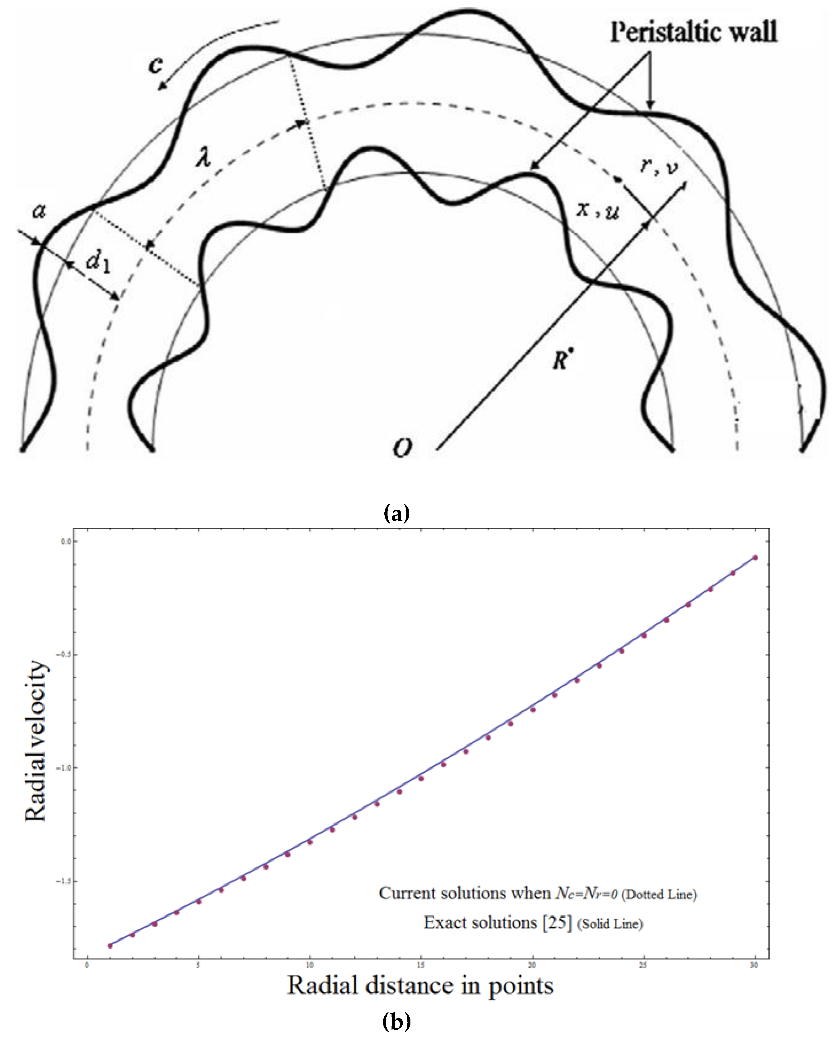
Abstract
:1. Introduction
2. Mathematical Modeling
3. Solution of the Problem
4. Graphical Results and Discussion
5. Conclusions
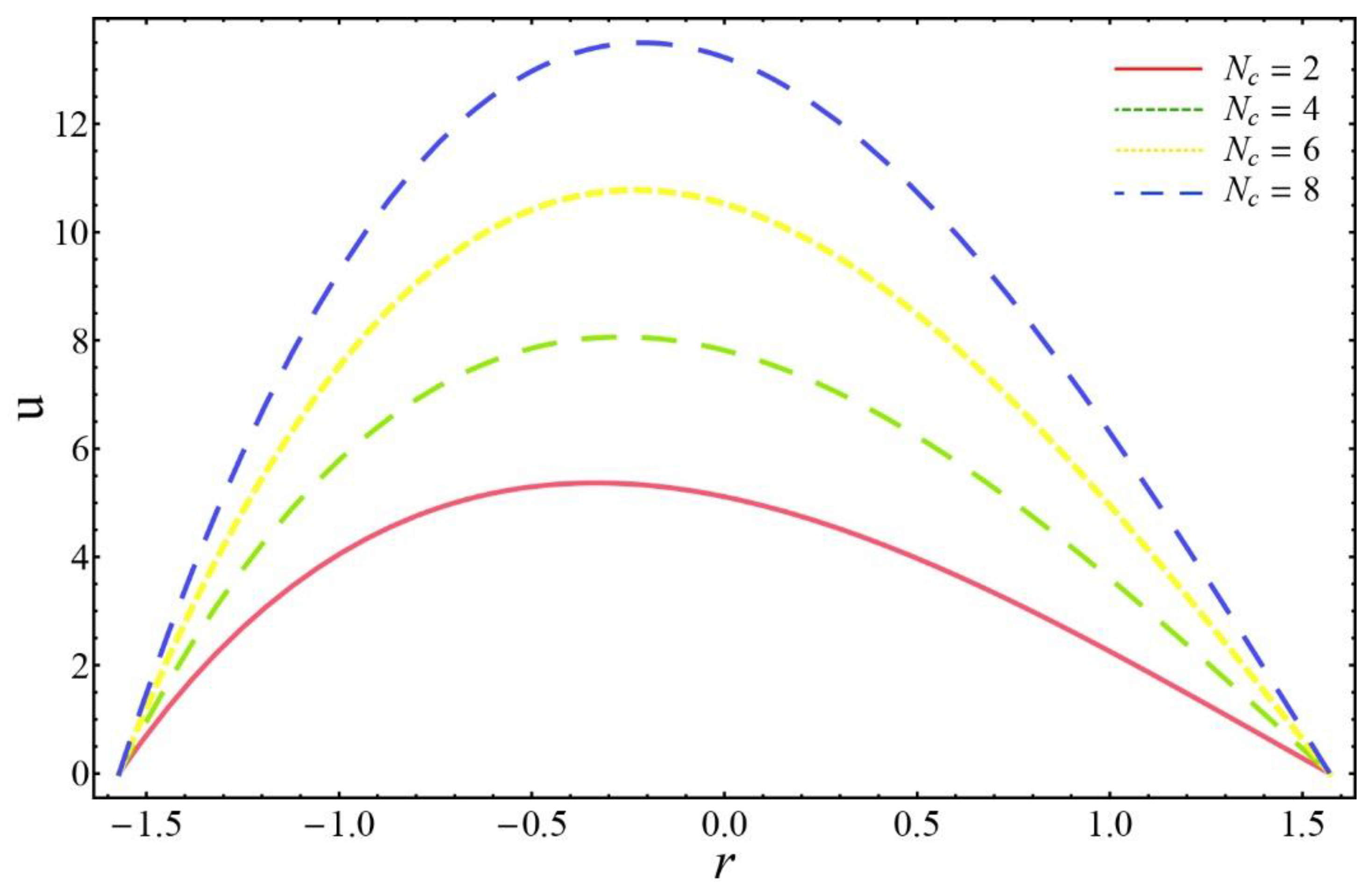
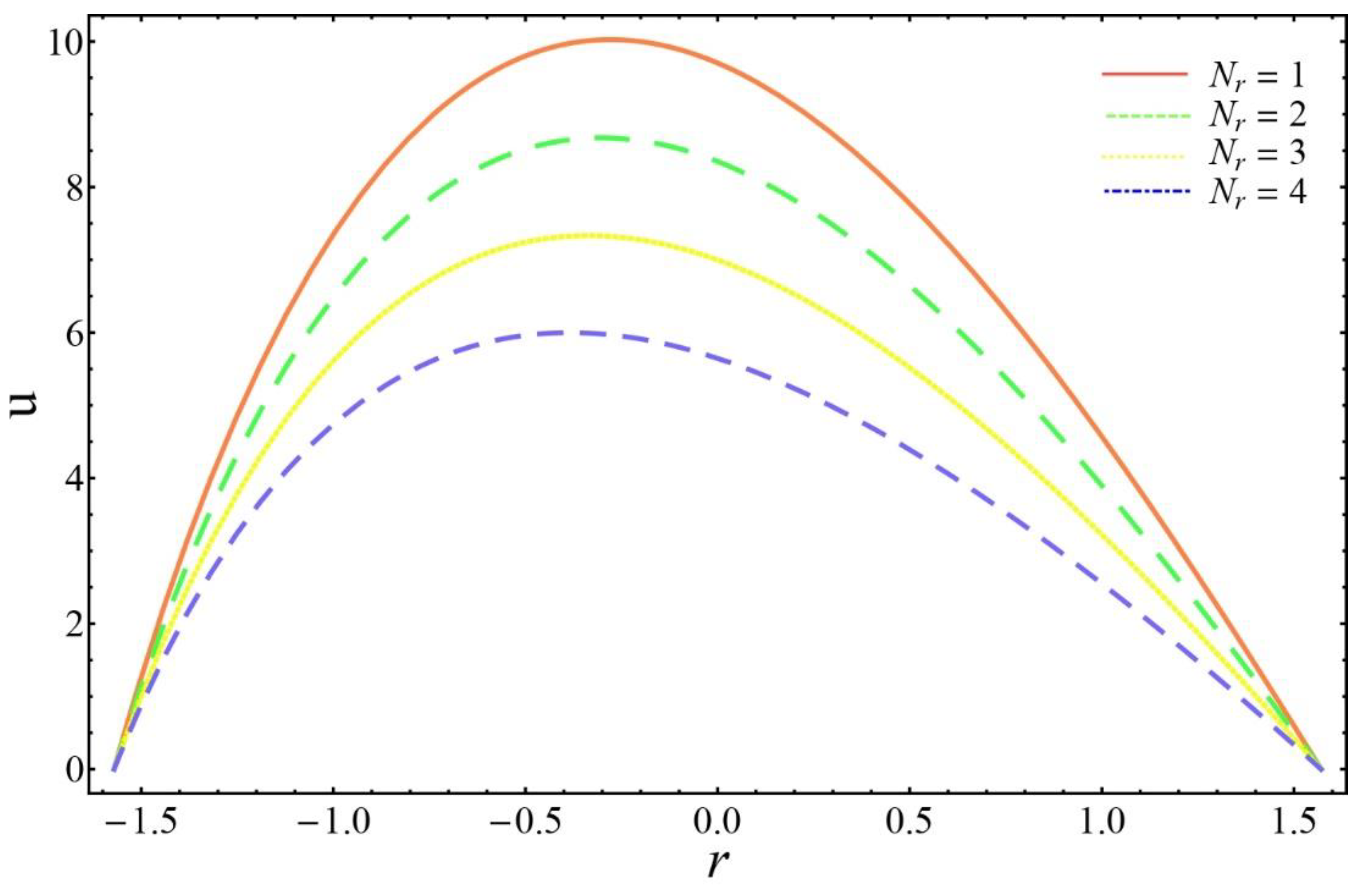
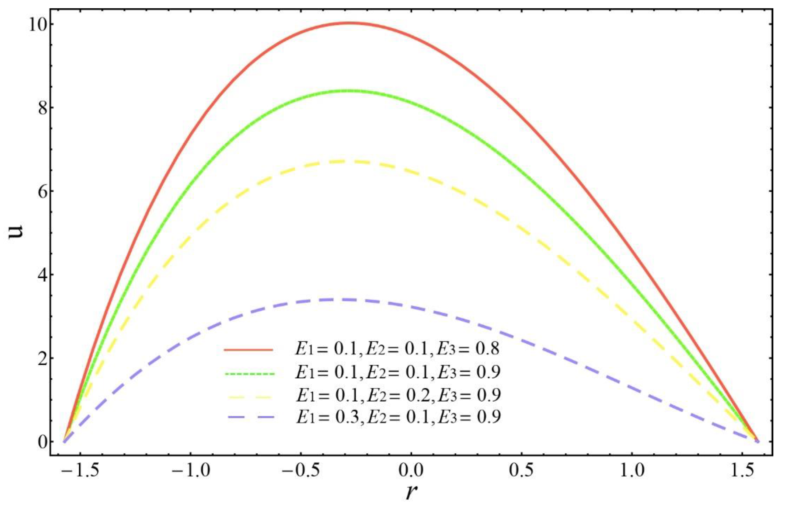
- The velocity profile increases with an increasing regular buoyancy ratio, but buoyancy parameter and compliant walls give opposite effects on velocity.
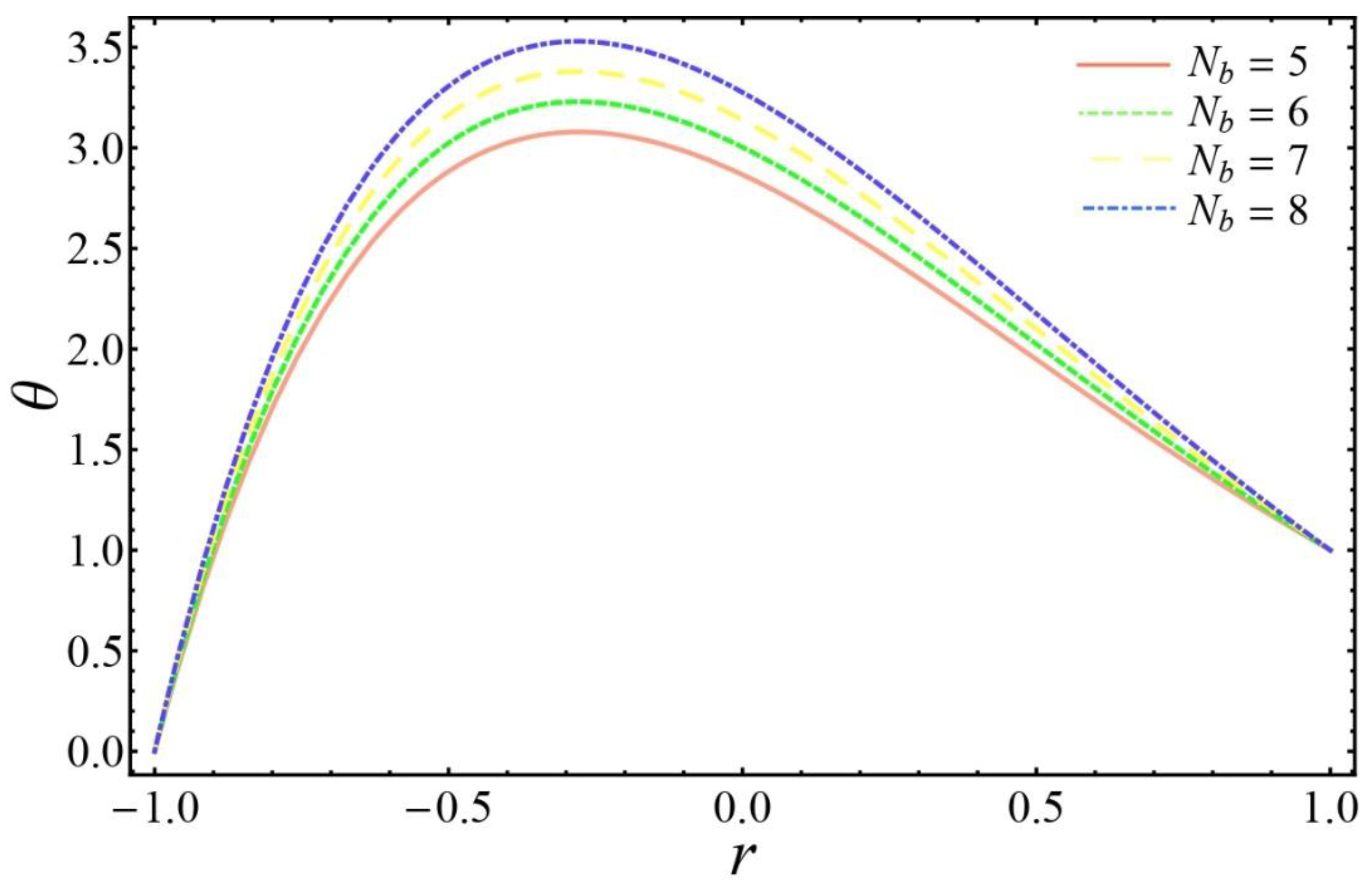
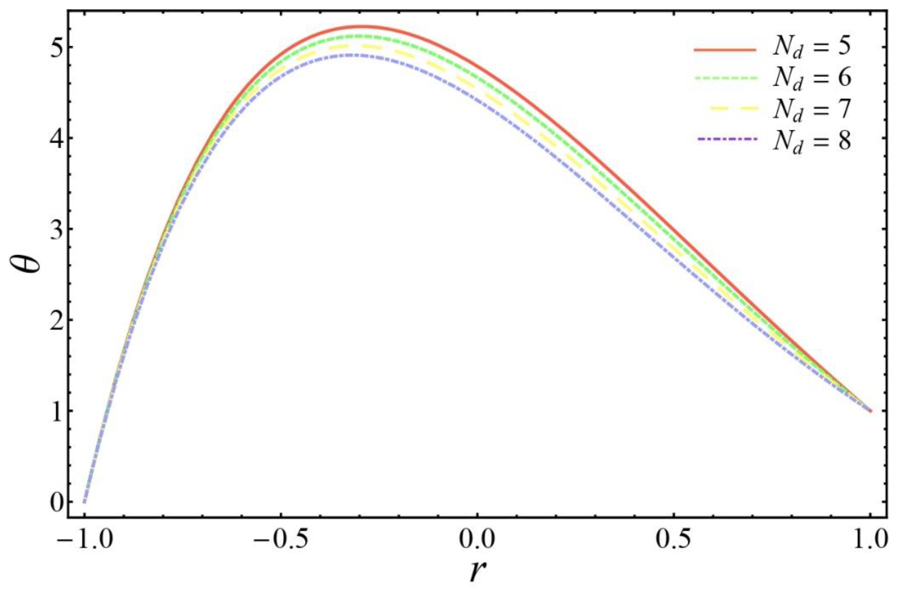
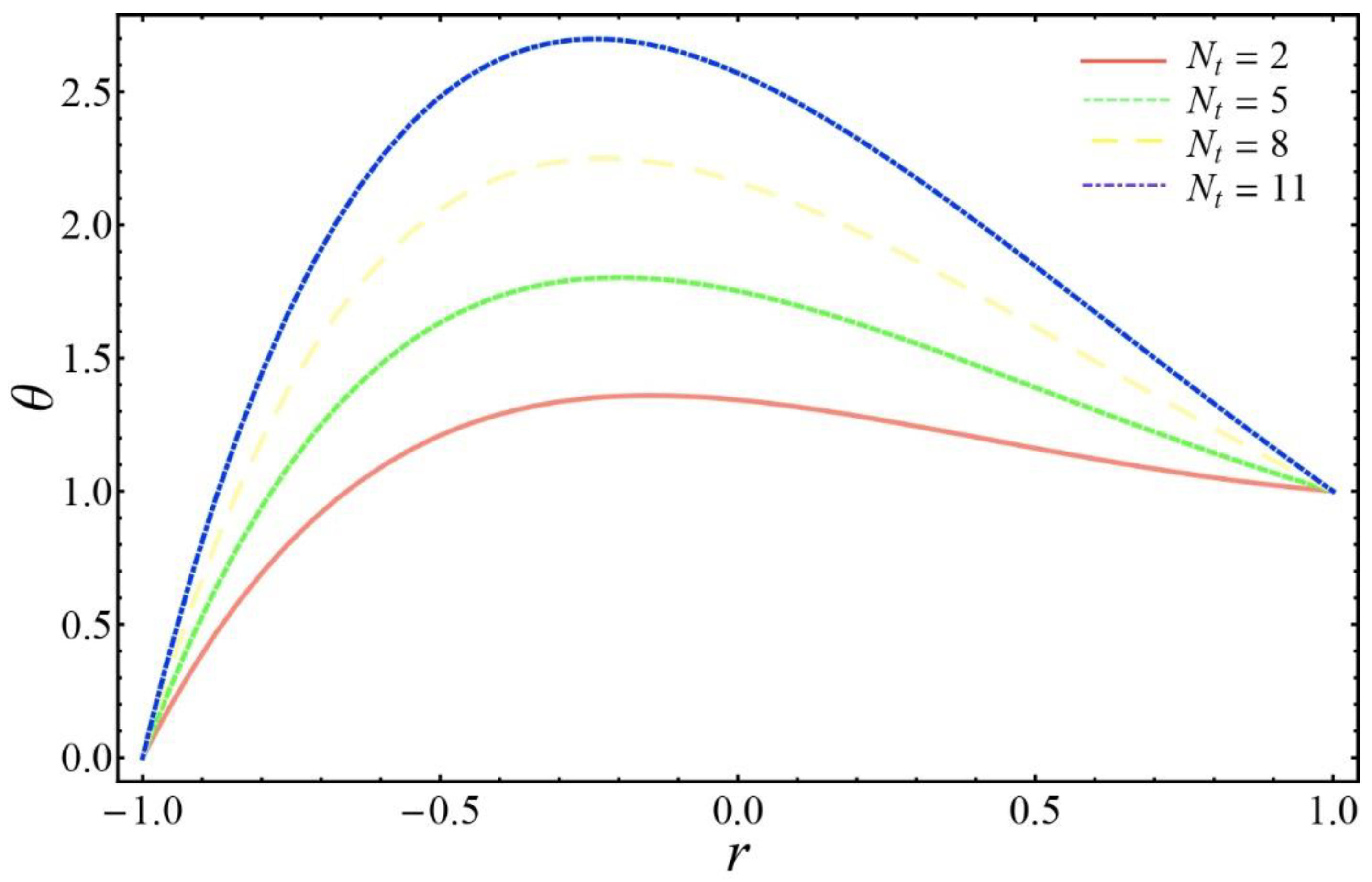
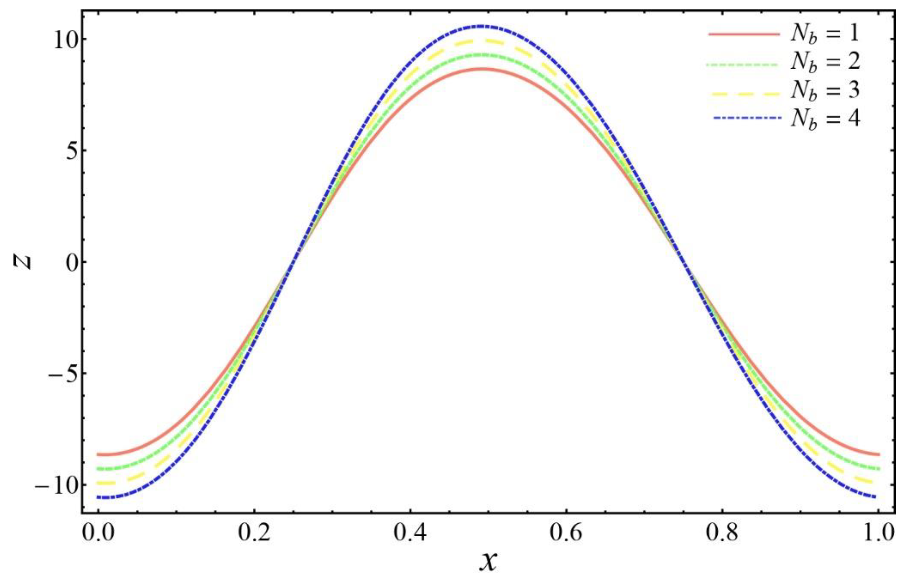
- The temperature increases with the Brownian motion parameter and thermophoresis parameter, but decreases with the buoyancy parameter. It is also noticed that the maximum temperature is observed in the center of the channel.
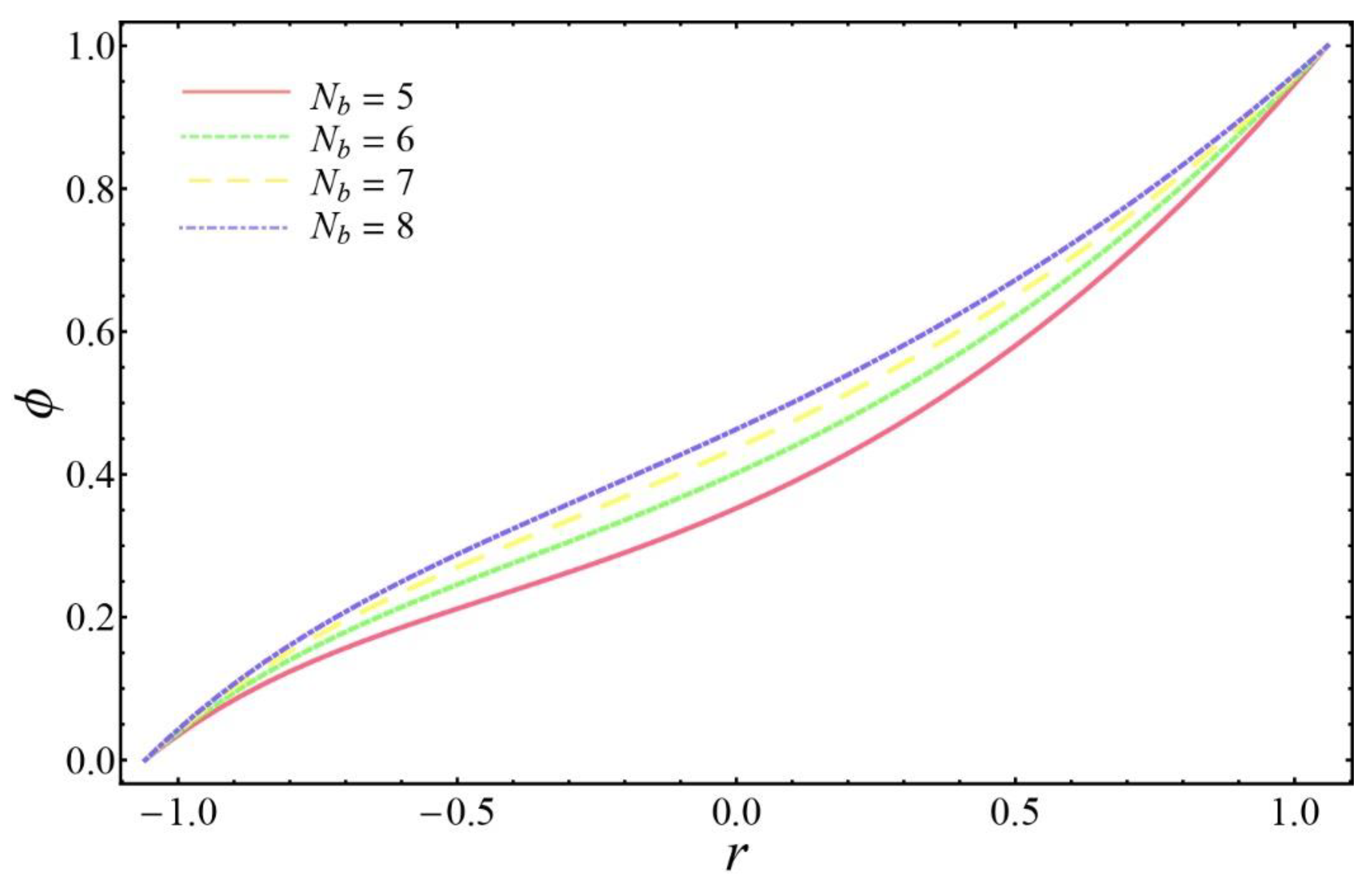
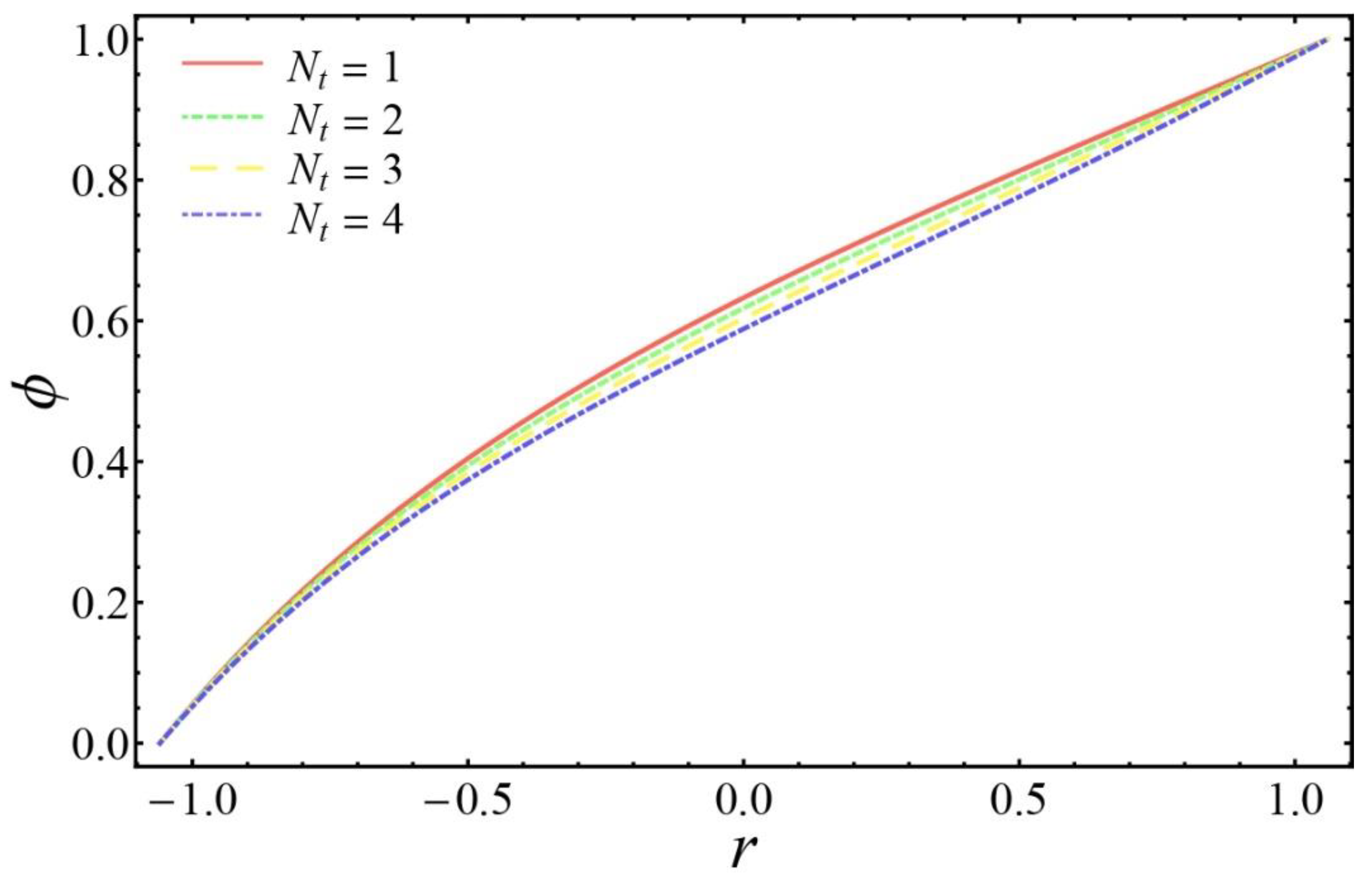
- The nanoparticles increase with the variation of regular buoyancy parameter, but decrease with increasing thermophoresis parameter. Moreover, it is concluded that in the center, there are fewer numbers of nanoparticles as compared to the left side boundary.
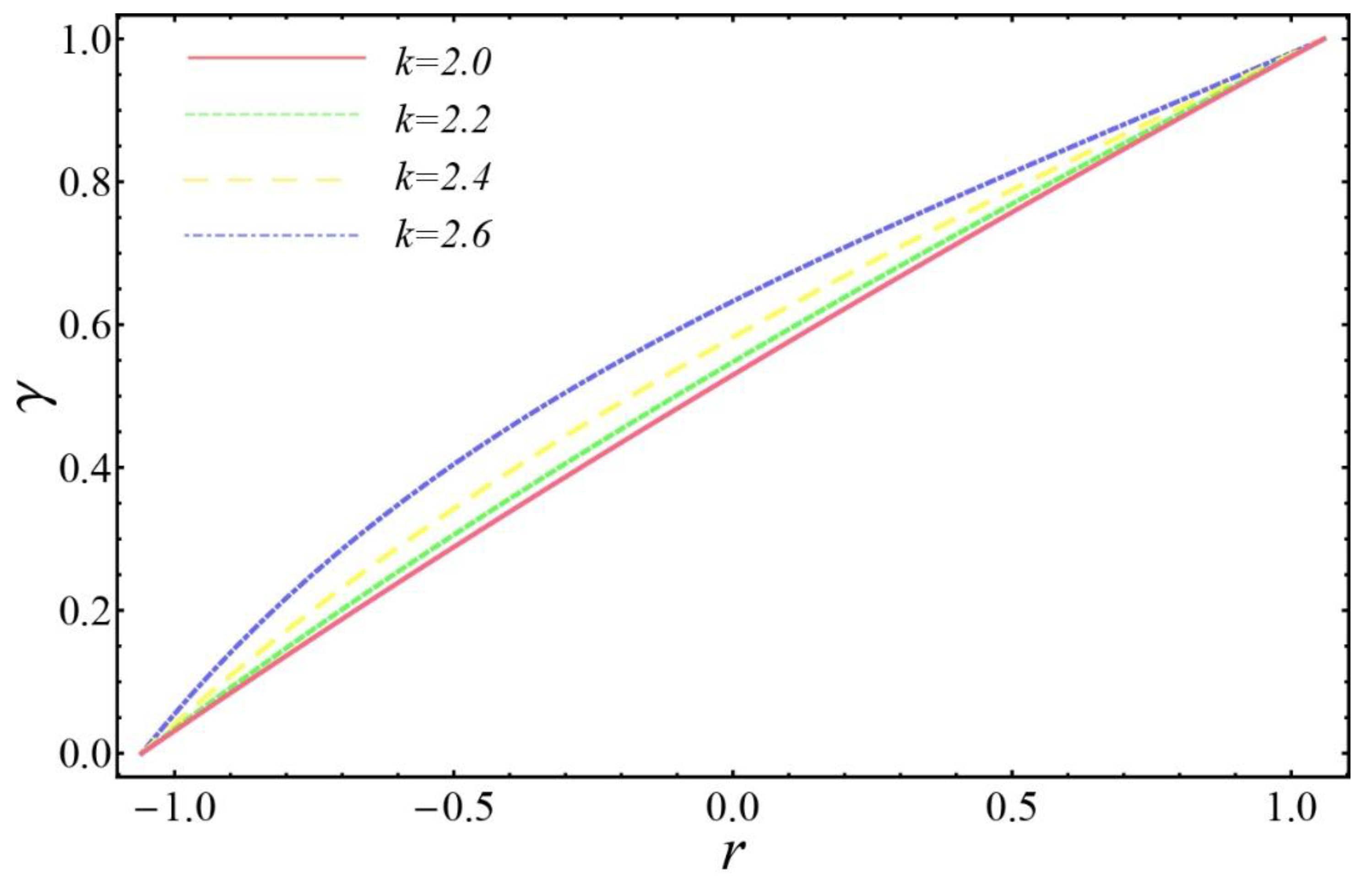
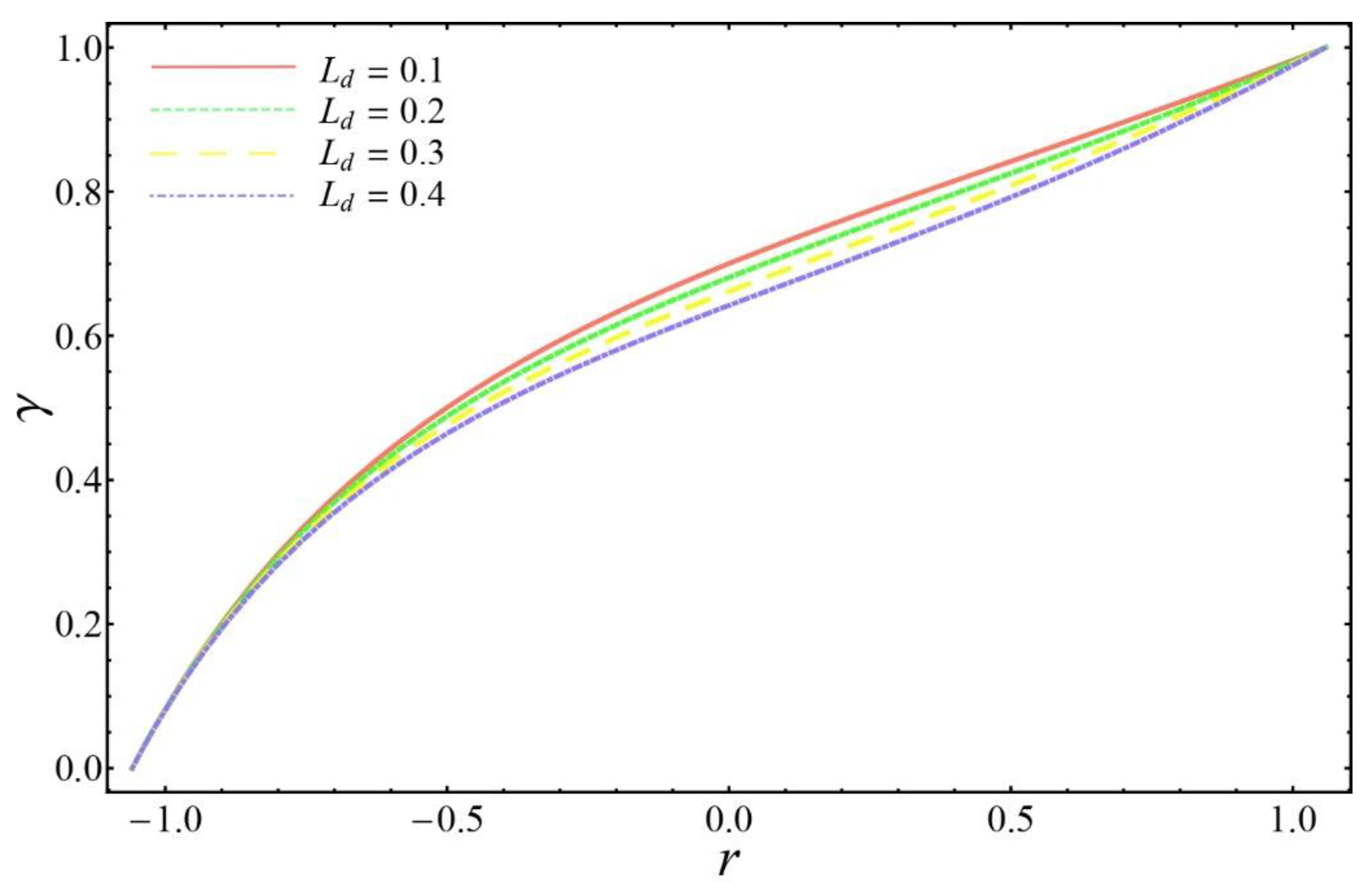
- It is observed that as an increase in the curvature of the channel, solutal concentration is increased, but reveals opposite behavior with Defour-Solutal Lewis number.
- It is found that heat is transferred in large amounts while increasing a modified Dufour parameter, but the less heat transfer is observed in case of Brownian motion parameter and thermophoresis parameter.
- It is disclosed that current analytical study is in line with the study [25] having exact solutions by skipping the terms of double diffusion.
Author Contributions
Funding
Conflicts of Interest
Appendix A
References
- Xiao, B.; Wang, W.; Zhang, X.; Long, G.; Fan, J.; Chen, H.; Deng, L. A novel fractal solution for permeability and Kozeny-Carman constant of fibrous porous media made up of solid particles and porous fibers. Powder Technol. 2019, 349, 92–98. [Google Scholar] [CrossRef]
- Xiao, B.; Zhang, X.; Giang, G.; Long, G.; Wang, W.; Zhang, Y.; Liu, G. Kozeny–Carman Constant For Gas Flow Through Fibrous Porous Media By Fractal-Monte Carlo Simulations. Fractals 2019, 27, 1950062. [Google Scholar] [CrossRef]
- Liang, M.; Liu, Y.; Xiao, B.; Yang, S.; Wang, Z.; Han, H. An analytical model for the transverse permeability of gas diffusion layer with electrical double layer effects in proton exchange membrane fuel cells. Int. J. Hydrog. Energy 2018, 43, 17880–17888. [Google Scholar] [CrossRef]
- Choi, S.U.S. Enhancing Thermal Conductivity of Fluids with Nanoparticles. In Proceedings of the ASME International Mechanical Engineering Congress and Exposition, Washington, DC, USA, 12–17 November 1995; Volume 66, pp. 99–105. [Google Scholar]
- Safaei, M.R.; Togun, H.; Vafai, K.; Kazi, S.N.; Badarudin, A. Investigation of Heat Transfer Enhancement in a Forward-Facing Contracting Channel Using FMWCNT Nanofluids. Numer. Heat Transf. Part A Appl. 2014, 66, 1321–1340. [Google Scholar] [CrossRef]
- Zeeshan, A.; Ellahi, R.; Mabood, F.; Hussain, F. Numerical study on bi-phase coupled stress fluid in the presence of Hafnium and metallic nanoparticles over an inclined plane. Int. J. Numer. Methods Heat Fluid Flow 2019, 2854–2869. [Google Scholar] [CrossRef]
- Ibrahim, W.; Makinde, O.D. Double-diffusive mixed convection and MHD stagnation point flow of nanofluid over a stretching sheet. J. Nanofluids 2015, 4, 1–10. [Google Scholar] [CrossRef]
- Maskeen, M.M.; Zeeshan, A.; Mehmood, O.U.; Hassan, M. Heat transfer enhancement in hydromagnetic alumina–copper/water hybrid nanofluid flow over a stretching cylinder. J. Therm. Anal. Calorim. 2019, 138, 1127–1136. [Google Scholar] [CrossRef]
- Ellahi, R. The effects of MHD and temperature dependent viscosity on the flow of non-Newtonian nanofluid in a pipe: Analytical solutions. Appl. Math. Model. 2013, 37, 1451–1467. [Google Scholar] [CrossRef]
- Abd Elnaby, M.A.; Haroun, M.H. A new model for study the effect of wall properties on peristaltic transport of a viscous flui. Commun. Nonlinear Sci. Numer. Simul. 2008, 13, 752–762. [Google Scholar] [CrossRef]
- Mittra, T.K.; Prasad, S.N. On the influence of wall properties and Poiseuille flow in peristalsis. J. Boimech. 2018, 6, 81–693. [Google Scholar] [CrossRef]
- Srivastava, V.P.; Srivastava, L.M. Influence of wall elasticity and poiseuille flow induced by peristaltic induced flow of a particle-fluid mixture. Int. J. Eng. Sci. 1997, 35, 799–825. [Google Scholar] [CrossRef]
- Muthu, P.; Kumar, B.V.R.; Chandra, P. Peristaltic motion of micropolar fluid in circular cylindrical tubes: Effect of wall properties. Appl. Math. Model. 2008, 32, 2019–2033. [Google Scholar] [CrossRef]
- Nadeem, S.; Maraj, E.N.; Akbar, N.S. Investigation of peristaltic flow of Williamson nanofluid in a curved channel with compliant walls. Appl. Nanosci. 2014, 4, 511. [Google Scholar] [CrossRef] [Green Version]
- Hassan, M.; Marin, M.; Alsharif, A.; Ellahi, R. Convective heat transfer flow of nanofluid in a porous medium over wavy surface. Phys. Lett. A 2018, 382, 2749–2753. [Google Scholar] [CrossRef]
- Ellahi, R.; Zeeshan, A.; Hussain, F.; Asadollahi, A. Peristaltic blood flow of couple stress fluid suspended with nanoparticles under the influence of chemical reaction and activation energy. Symmetry 2019, 11, 276. [Google Scholar] [CrossRef] [Green Version]
- Riaz, A.; Alolaiyan, H.; Razaq, A. Convective Heat Transfer and Magnetohydrodynamics across a Peristaltic Channel Coated with Nonlinear Nanofluid. Coatings 2019, 9, 816. [Google Scholar] [CrossRef] [Green Version]
- Bég, O.A.; Tripathi, D. Mathematica simulation of peristaltic pumping with double-diffusive convection in nanofluids: A bio-nano-engineering model. J. Nanoeng. Nanosyst. 2011, 225, 99–114. [Google Scholar]
- Akbar, N.S.; Maraj, E.N.; Butt, A.W. Copper nanoparticles impinging on a curved channel with compliant walls and peristalsis. Eur. Phys. J. Plus 2014, 129, 183. [Google Scholar] [CrossRef]
- Bhatti, M.M.; Rashidi, M.M. Effects of thermo-diffusion and thermal radiation on Williamson nanofluid over a porous shrinking/stretching sheet. J. Mol. Liq. 2016, 221, 567–573. [Google Scholar] [CrossRef]
- Kuznetsov, A.V.; Nield, D.A. Double-diffusive natural convective boundary-layer flow of a nanofluid past a vertical plate. Int. J. Therm. Sci. 2011, 50, 712–717. [Google Scholar] [CrossRef]
- Akbar, N.; Khan, Z.; Nadeem, S.; Khan, W. Double-diffusive natural convective boundary-layer flow of a nanofluid over a stretching sheet with magnetic field. Int. J. Numer. Methods Heat Fluid Flow 2016, 26, 108–121. [Google Scholar] [CrossRef]
- Akram, S.; Zafar, M.; Nadeem, S. Peristaltic transport of a Jeffrey fluid with double-diffusive convection in nanofluids in the presence of inclined magnetic field. Int. J. Geom. Methods Mod. Phys. 2018, 15, 1850181. [Google Scholar] [CrossRef]
- Akbar, N.S.; Habib, M.B. Peristaltic pumping with double diffusive natural convective nanofluid in a lopsided channel with accounting thermophoresis and Brownian moment. Microsyst. Technol. 2019, 25, 1217. [Google Scholar] [CrossRef]
- Hayat, T.; Hina, S.; Awatif, A.H.; Asghar, S. Effect of wall properties on the peristaltic flow of a third grade fluid in a curved channel with heat and mass transfer. Int. J. Heat Mass Transf. 2011, 54, 5126–5136. [Google Scholar] [CrossRef]
- Abbas, A.; Bai, Y.; Rashidi, M.M.; Bhatti, M.M. Analysis of Entropy Generation in the Flow of Peristaltic Nanofluids in Channels With Compliant Walls. Entropy 2016, 18, 90. [Google Scholar] [CrossRef]
- Srinivas, S.; Kothandapani, M. The influence of heat and mass transfer on MHD peristaltic flow through a porous space with compliant walls. Appl. Math. Comput. 2009, 213, 197–208. [Google Scholar] [CrossRef]
- Bhatti, M.M.; Ellahi, R.; Zeeshan, A. Study of Variable Magnetic Field on The Peristaltic Flow of Jeffrey Fluid in A Non-Uniform Rectangular Duct Having Compliant Walls. J. Mol. Liq. 2016, 222, 101–108. [Google Scholar] [CrossRef]
- Bhatti, M.M.; Ellahi, R.; Zeeshan, A.; Marin, M.; Ijaz, N. Numerical study of heat transfer and Hall current impact on peristaltic propulsion of particle-fluid suspension with compliant wall properties. Mod. Phys. Lett. B 2019, 33, 1950439. [Google Scholar] [CrossRef]
- He, J.H. Homotopy perturbation method for solving boundary value problems. Phys. Lett. A 2006, 350, 87–88. [Google Scholar] [CrossRef]


© 2020 by the authors. Licensee MDPI, Basel, Switzerland. This article is an open access article distributed under the terms and conditions of the Creative Commons Attribution (CC BY) license (http://creativecommons.org/licenses/by/4.0/).
Share and Cite
Alolaiyan, H.; Riaz, A.; Razaq, A.; Saleem, N.; Zeeshan, A.; Bhatti, M.M. Effects of Double Diffusion Convection on Third Grade Nanofluid through a Curved Compliant Peristaltic Channel. Coatings 2020, 10, 154. https://doi.org/10.3390/coatings10020154
Alolaiyan H, Riaz A, Razaq A, Saleem N, Zeeshan A, Bhatti MM. Effects of Double Diffusion Convection on Third Grade Nanofluid through a Curved Compliant Peristaltic Channel. Coatings. 2020; 10(2):154. https://doi.org/10.3390/coatings10020154
Chicago/Turabian StyleAlolaiyan, Hanan, Arshad Riaz, Abdul Razaq, Neelam Saleem, Ahmed Zeeshan, and Muhammad Mubashir Bhatti. 2020. "Effects of Double Diffusion Convection on Third Grade Nanofluid through a Curved Compliant Peristaltic Channel" Coatings 10, no. 2: 154. https://doi.org/10.3390/coatings10020154