Article

Buoyancy Driven Flow with Gas-Liquid Coatings of Peristaltic Bubbly Flow in Elastic Walls

1
Department of Mathematics and Statistics, University of Lahore Sargodha Campus, Sargodha 40100, Pakistan
2
Department of Mathematics, Division of Science and Technology, University of Education, Lahore 54770, Pakistan
3
Department of Mathematics & Statistics, Faculty of Basic and Applied Sciences (FBAS), International Islamic University, Islamabad 44000, Pakistan
4
Center for Modeling and Computer Simulation, Research Institute, King Fahd University of Petroleum & Minerals, Dhahran-3126, Saudi Arabia
5
Fulbright Fellow, Department of Mechanical Engineering, University of California Riverside, Riverside, CA 92521, USA
6
Center for Communications and IT Research, Research Institute, King Fahd University of Petroleum & Minerals, Dhahran-31261, Saudi Arabia
*
Author to whom correspondence should be addressed.
Coatings 2020, 10(2), 115; https://doi.org/10.3390/coatings10020115
Submission received: 4 November 2019 / Revised: 22 January 2020 / Accepted: 26 January 2020 / Published: 30 January 2020
(This article belongs to the Special Issue Recent Trends in Coatings and Thin Film–Modeling and Application)

Abstract

:
In this paper, liquid coatings of bubbly flow with peristaltic motion inside elastic walls is investigated. The proposed model is constructed using the two-fluid approach with the most distinctive collaboration among gas, fluid, pressure, and drag forces. Variation in pressure leads to a change in void fraction. The differential controlling conditions affected by the long wavelength of the peristaltic wave and the slow movement are taken into account. Analytical results of the simplified governing equations are obtained using the homotopy perturbation method (HPM). The features of the significant parameters are shown and examined graphically.

1. Introduction

An air-pocket-incited gas-fluid stream is the premise of smooth motion in numerous compound building gadgets and applications ranging from boilers or evaporators and more than a few stage bubble segment reactors of different structures to enormous-scale vigorous (and sometimes anaerobic) sewage treatment plants. The two-phase transport hypothetical talk and test request are firmly connected. On the other hand, the amalgamation that emerges from this association creates colossal innovative potential for estimations advising and approving unique models. The subsequent innovation develops utility in an expansive range of uses, from cutting-edge atomic hardware and space motors to pharmaceutical assembling, nourishment innovation, vitality, and natural remediation. Sussman et al. [1] considered a level-set methodology for figuring out answers for a incompressible two-stage stream. Their study was about the movement of air bubbles in the water and falling water drops in the air. A single-liquid model for a two-stage stream with variable thickness to the stream-water flow was analyzed by Bankoff [2]. Zuber and Findlay [3] estimated the normal volumetric fixation in two-stage stream frameworks. In their analysis, the outcomes anticipated by the investigation were contrasted with experimental data acquired for different two-phase stream systems, with different fluid gas blends in the adiabatic, vertical stream over a wide weight territory. Picchi and Poesio [4] developed a unified model for both horizontal and slightly inclined fluid pipes lubricated with two-phase gas/shear-thinning fluid. Sato and Sekoguchi [5] suggested the velocity distribution of liquid in two-phase bubble flow. A more precise analytical procedure was constructed that created the justified foreboding of the liquid velocity dispensation in two-phase bubble flow. Kuwagi et al. [6] investigated the oscillation of bubbly flow through a normally placed cylinder employing a tridimensional system. Picchi and Battiato [7] discussed immiscible two-phase flow in porous media and elaborated the impact of pore-scale flow. Bonzanini et al. [8] simulated 1-D slug and stratified flow in pipes. Sontti and Atta [9] investigated co-flow in microchannels to discuss the viscous effect on Taylor bubble formation. Bhatti et al. [10] broke down the heat and mass exchange of a two-phase stream with an electric twofold layer whose impacts were incited due to the peristaltic impetus within the sight of the transverse attractive field. Haider et al. [11] presented the heat transfer as well as a magnetic field investigation on the peristaltically initiated movement of tiny particles.
Moreover, the mechanism of peristalsis comprises expansion and contraction events that impel an ingredient forward. Examples of some cases of the peristaltic phenomenon are the transport of bile in the bile duct, the transport of urine from the kidney to the gallbladder, the transport of cilia, the vasomotion of small blood vessels, and the mixing of food in the digestive tract, to name a few. The peristaltic phenomenon also has several industrial applications such as in the flow in tube pumps, in the rollers and hoses in heart-lung machines, and in the dialysis process during open-heart surgery. [12,13].
Furthermore, in buoyancy-driven flows, although the difference in inertia is almost negligible, the gravity remains sufficiently strong to make the specific weight significantly different during the flow in multiphase fluids. Tripathi et al. [14] investigated buoyancy effects in the peristaltic flow of nanofluid under the influence of electro-osmosis. Animasaun and Pop [15] numerically explored the effects of buoyancy on the flow driven by catalytic surface reactions. Angirasa et al. [16] reported the buoyancy effects in a fluid saturated with a porous medium. Rashidi et al. [17] studied fluid flow in the presence of buoyancy forces.
In addition to the above, the presence of bubbles has appeared in several applications in a gas-liquid flow. Many theoretical and numerical investigations have been conducting for multiphase bubbly flows in oil, gas, and liquid. It has numerous usages, such as in optical fiber sensing applications [18], sensitive pressure measurement [19], the human bloodstream during decompression sickness, and subcooled flow boiling in macro-channels [20]. Ellhi et al. [21] examined the simulation of bubble through the nozzle of tube. Furthermore, lubricated coatings with bubbles in peristaltic motion have a lot of applications in the biomedical field, and among several of these, in the control of blood pressure. Particle coating with viscous liquids is an essential component in the industry for surface modification purposes in order to induce and improve precise functionalities. Coating with viscous liquids is usually present in very rich industrial trials, which allow the coating of particles under the shear forces exerted in a mixing device. A list of key investigations on peristaltic flows [22,23,24], multiphase flows [25,26,27,28,29], bubbly flows [30,31,32,33,34], coatings [35,36,37,38,39,40], elastic medium [41,42], and several other references are available, which provide a more in-depth understanding to the reader.
Due to the immense contribution of two-phase flow structures in many significant fields, this study attempts to trap the structures of gas-liquid bubbly flow inside the elastic walls under the peristaltic mechanism applied over a two-fluid model. Due to the nonlinear model, a powerful and efficient technique called the homotopy perturbation method is used for finding analytic solutions. This method works even without the need of a linearization process of nonlinear differential equations. The parameters affecting the flow prominently have been examined with the help of a graphical illustration.

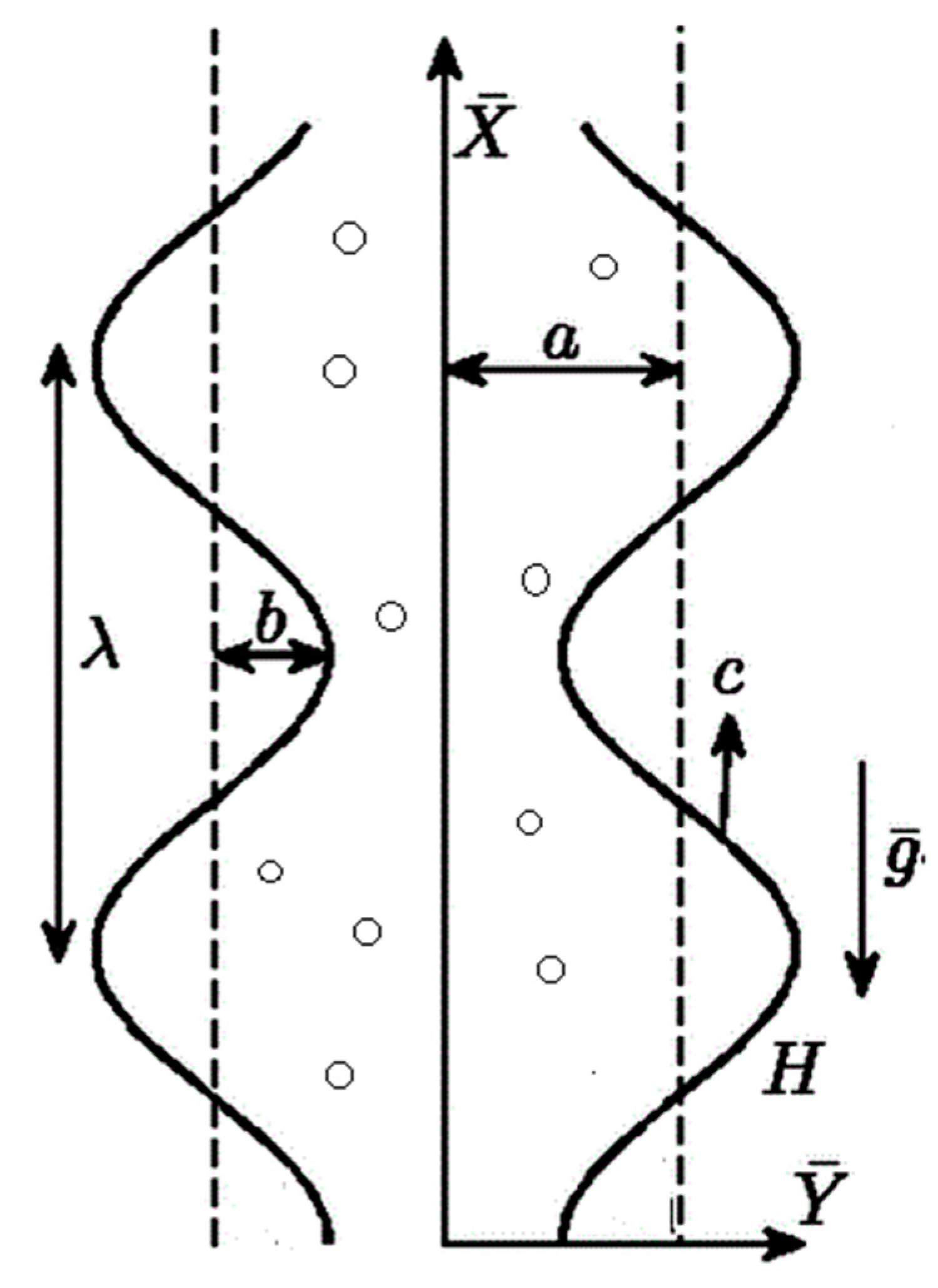
2. Mathematical Formulation

We assumed a symmetric channel with flexible walls starting at the origin of a rectangular coordinate system, see Figure 1. Plates were placed parallel to the x-axis, on either side of the origin, separated by a distance of 2h. Only the upper portion of the symmetric channel was taken into consideration. A continuous wave with long wavelength, λ, and speed, c, traveled on the plates [43] and was defined by
z = h ( X , t ) = a ( 1 + η ( X , t ) )
where η ( x , t ) = ϕ S i n ( 2 π λ ( X c t ) ) , ϕ = b a having an interval of ( 0 , 1 ) .

Two-Fluid Model

The two-fluid model for the flow of the gas bubbles in the Newtonian fluid with the Euler–Euler model was employed. Both phases were considered as a continuum and could be defined with the help of differential equations. A thin surface separated both the fluids and at the interphase, and consequently a jump continuity condition could be employed [44]. The bubbles were distributed homogenously in the flow and considered to be of the same spherical shape. It was assumed that no mass was transferred between the two phases and isothermal conditions were maintained. The density of the liquid was constant, whereas for the gas-phase it depended on pressure, p. Bubble redispersion was neglected and there was low gas holdup. With these assumptions, continuity equations for both the liquid and bubble phase were of the form [45]
. ( U l ) = 0 ,
( ε g ρ g ) t + . ( ε g ρ g U g ) = 0 ,
where Ul and Ub were the liquid and bubble velocities, respectively, whereas εg and ρg represented the void space and density of the gaseous phase with the closure relation constraint ε l + ε g = 1 . For low gas ε l 1 . Using ideal gas laws, ρ g = p RT 0 , ρ l constant , and because isothermal conditions were taken into account T0 remained constant.
The momentum transfer for both the liquid and gaseous phase [46] were defined as
ρ l ( U l t + U l U l X + V l U l Y ) = P X + μ ( 2 U l X 2 + 2 U l Y 2 ) + ρ l g ε g ρ l g ,
ρ l ( V l t + U l V l X + V l V l Y ) = P Y + μ ( 2 V l X 2 + 2 V l Y 2 ) ,
ε g ρ g ( U g t + U g U g X + V g U g Y ) = ε g P X + μ ε g ( 2 U g X 2 + 2 U g Y 2 ) + ρ g g ε g F int , x ,
ε g ρ g ( V g t + U g V g X + V g V g Y ) = ε g P Y + μ ε g ( 2 V g X 2 + 2 V g Y 2 ) F int , y ,
where Fint is the interaction force between the liquid and gaseous phases. These forces were able to be divided into three parts―i) force due to drag, which is incorporated in the uniform flow, ii) added mass force due to the acceleration of the bubble, and iii) lift force for the spherical bubble [47]. Mathematically this could be written as
F int = F d + F a m + F l ,
F d = C w V b ( U b U l ) ,
F a m = C a m V b ρ l ( d U s l i p d t ) ,
F l = C l V b ρ l ( U b U l ) × ( × U l ) ,
in which Cw was a constant involving bubble diameter and drag force, Vb was the volume of the bubble, Cam was a constant related to the volume fraction of liquid accelerated with the bubble, Uslip was slip velocity defined as U s l i p = U b U l , and Cl was the lift coefficient. Finally, Ub was the speed of a single bubble and it was related to gas velocity by U g = U b + U d r i f t , where U d r i f t is the average drift velocity, which was proportional to the ratio of the special change in gas void fraction to total void fraction of gas.
To transform from a fixed frame to wave frame, Lorentz transformations were employed.
X = x * c t ,   Y = y * ,   U = u * c ,   V = v * , p * ( x * ,   y * ) = P ( X , Y ,   t ) .
Equations (2)‒(11) became
. ( u l * ) = 0 ,
c ( ε g ρ g ) x * + . ( ε g ρ g u g * ) = 0 ,
ρ l ( u l * u l * x * + v l * u l * y * ) = p x * + μ ( 2 u l * x * 2 + 2 u l * y * 2 ) + ( 1 ε g ) ρ l g ,
ρ l ( u l * v l * x * + v l * v l * y * ) = p y * + μ ( 2 v l * x * 2 + 2 v l * y * 2 ) ,
ε g ρ g ( u g * u g * x * + v g * u g * y * ) = ε g p x * + μ ε g ( 2 u g * x * 2 + 2 u g * y * 2 ) + ρ g g ε g f int , x ,
ε g ρ g ( u g * v g * x * + v g * v g * y * ) = ε g p * y * + μ ε g ( 2 v g * x * 2 + 2 v g * y * 2 ) f int , y ,
f int = f d + f a m + f l ,
f d = C w V b ( u b * u l * ) ,
F a m = C a m V b ρ l c ( u b * x u l * x + ( u b * ) u b * ( u l * ) u l * ) ,
F l = C l V b ρ l ( u b * u l * ) × ( × u l * ) ,
and by employing the dimensionless quantities were
x = x * λ , y = y * a , u l , g = u l , g * c , v l , g = v l , g * c , δ = a λ , Re = ρ c a μ , p = a 2 μ λ c P E o = a 2 σ ρ l g , R b e = a c μ ρ l V b , A = μ c σ .
By imposing Equation (23) on Equations (12)‒(22) and considering Re and δ approach zero, the corresponding expressions resulted in
ε g = c 1 ρ g u b ,
p x = 2 u l y 2 + ( 1 ε g ) E o A ,
A ρ l p x = E o ( ρ g + V b C w g ) R b e A ρ l ( C l W s u l z + C a m W s ( u b u l ) y ) ,
along with the consequential nondimensional boundary limitations
u l ( h ) = 0 , u l ( h ) = 0 , ε g ( 0 ) = 1 .

3. Mathematical Solutions and Results

To compute the solutions of complicated nonlinear coupled equations, a powerful and efficient technique called the homotopy perturbation method (HPM) was used for finding analytic solutions. HPM is a powerful method which works even without the need of a linearization process [48,49,50]. It tends to reduce the nonlinear equations into a system of linear equations and generates an asymptotic solution. To serve the purpose, the initial guess was formed as
u l , 0 = 1 2 ( 2 h 2 P + P y 2 )   a n d   u b , 0 = 1 + P y .
The linear operators were
L 1 = d 2 u l d y 2 ,   a n d   L 2 = d u b d y .
From Equations (22)‒(23)
E q 1 ( x , y , q ) = P ( x , q ) 2 u l y 2 ( x , y , q ) ( 1 c 1 ρ l u b ( x , y , q ) ) E o A ,
E q 2 ( x , y , q ) = A ρ l P ( x , q ) + E o ( ρ g ( x , y , q ) + V b C w g ) R b e A ρ l ( C l W s u l ( x , y , q ) z + C a m W s ( u b ( x , y , q ) u l ( x , y , q ) ) y ) ,
Constructing the homotopy that satisfy
H ( U , q ) = ( 1 q ) ( L 1 ( U ) L 2 ( u l , 0 ) ) + q ( E q 1 ( U ) ) = 0 ,
H ( V , q ) = ( 1 q ) ( L 2 ( V ) L 2 ( u b , 0 ) ) + q ( E q 2 ( V ) ) = 0 ,
with q ( 0 , 1 ) . When q = 0, the equation provided an initial guess, and for q = 1 the equation generated a required solution. The solution should be of the form
U = U 0 + p U 1 + ... ,   V = V 0 + p V 1 + ...
Setting p = 1 the solution will be
U = U 0 + U 1 + ... ,   V = V 0 + V 1 + ...
The expressions achieved up to second order were
u f = K 5 + K 6   y + K 7 y 2 + K 8 y 3 + K 9 y 4 K 10 y 5 , K 5 = 1 h 2 P 2 1 12 Eoh 4 P 2 1 24 C am Eoh 4 PR be W s + 1 24 C l Eoh 4 PR be W s C w Eo 2 h 4 PV b 24 g ρ l , K 6 = 1 3 Eo h 2 P 1 6 C a m Eo h 2 P R b e W s C w Eo 2 h 2 V b 3 g ρ l 3 C w Eo 2 h 4 P V b 40 g ρ l , K 7 = P 2 ,   K 8 = Eo P 3 + 1 6 C a m Eo P W s + C w Eo 2 V b 3 g ρ l + C w Eo 2 h 2 P V b 12 g ρ l , K 9 = Eo P 2 12 + 1 24 C a m Eo P R b e W s 1 24 C l Eo P R b e W s + C w Eo 2 P V b 24 g ρ l , K 10 = C w Eo 2 P V b 120 g ρ l
u b = 1 + K 11 y + K 12 y 2 + K 13 y 3 + K 14 y 4 , K 11 = 1 6 g ρ l ( 3 C w EoV b ( 4 + h 2 P ) ( 2 + C a m W s ) + g P ( 18 + C l Eo h 2 R b e W s C a m ( 18 + Eo h 2 R b e ) W s + 6 C a m 2 W s 2 ) ρ l ) K 12 = 1 12 g 2 ρ l 2 ( 3 C w 2 Eo 2 ( 4 + h 2 P ) V b 2 + C w Eo g P V b ( 18 + Eo h 2 + 12 C a m W s ) ρ l + 6 ( C a m C l ) g 2 P R b e W s ( 2 + C a m W s ) ρ l 2 ) , K 13 = 1 6 g 2 ρ l 2 ( Eo P ( C w 2 EoV b 2 + C w g V b ( 2 + C a m ( 1 + R b e ) W s C l R b e W s ) ρ l + ( C a m C l ) g 2 R b e W s ρ l 2 ) ) K 14 = C w Eo 2 P V b ( C w V b + g ρ l ) 24 g 2 ρ l 2 .
Here, P = p x . The flow rate in the fixed frame [51] was defined by
Q f = h h u f ( x , y ) d y ,
Q g = h h u g ( x , y ) d y ,
Q = Q f + Q g = h h u f ( x , y ) + u g ( x , y ) d y .
Solving the equation to get P in terms of Q and x was
p x = 1 4 E o g h 5 ρ l ( K 1 h 5 + K 2 h 3 ( K 1 h 5 + K 2 h 3 ) 2 ( K 3 h 5 + K 4 h 6 ) ) K 1 = E o ( C l g R b e W s ρ l C w A E o V b C a m g R b e W s ρ l ) , K 2 = 10 g ρ l A K 3 = 120 E o g 2 ρ l 2 A ( 1 Q ) , K 4 = 240 g 2 h ρ l 2 E o A

4. Discussion

To study the impact of numerous parameters, such as volume ( V b ) , Eotvos number ( E o ) , added mass coefficient ( C a m ) , slip velocity ( W s ) , lift coefficient ( C l ) , and model coefficient ( C w ) , Figure 2, Figure 3, Figure 4, Figure 5, Figure 6, Figure 7, Figure 8, Figure 9, Figure 10, Figure 11, Figure 12, Figure 13, Figure 14, Figure 15, Figure 16, Figure 17, Figure 18 and Figure 19 were plotted.

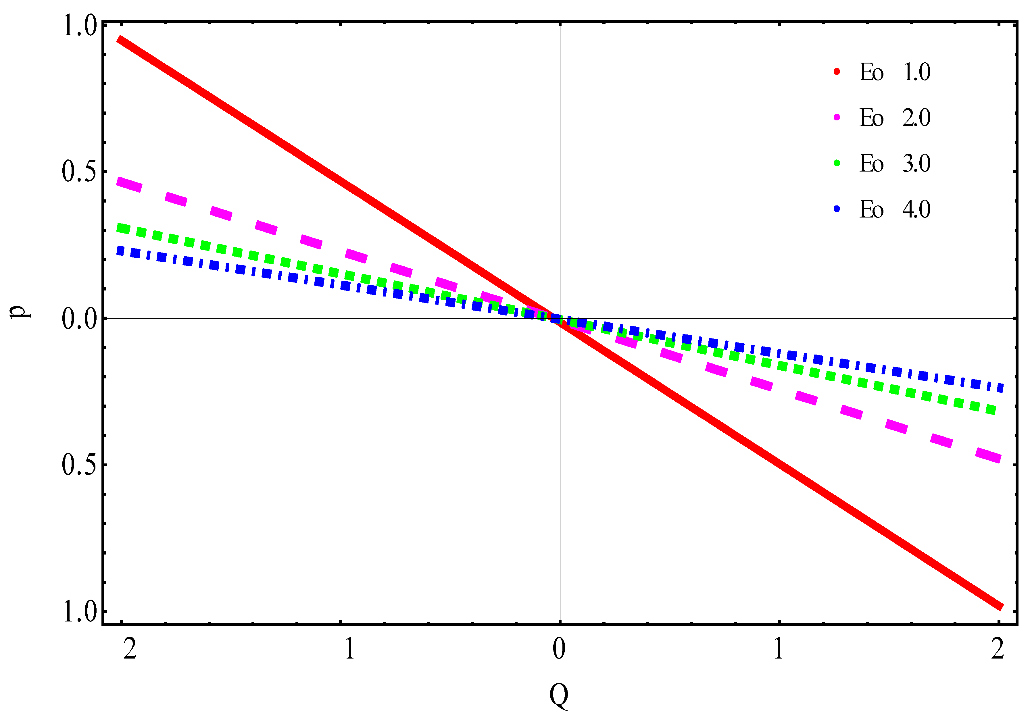
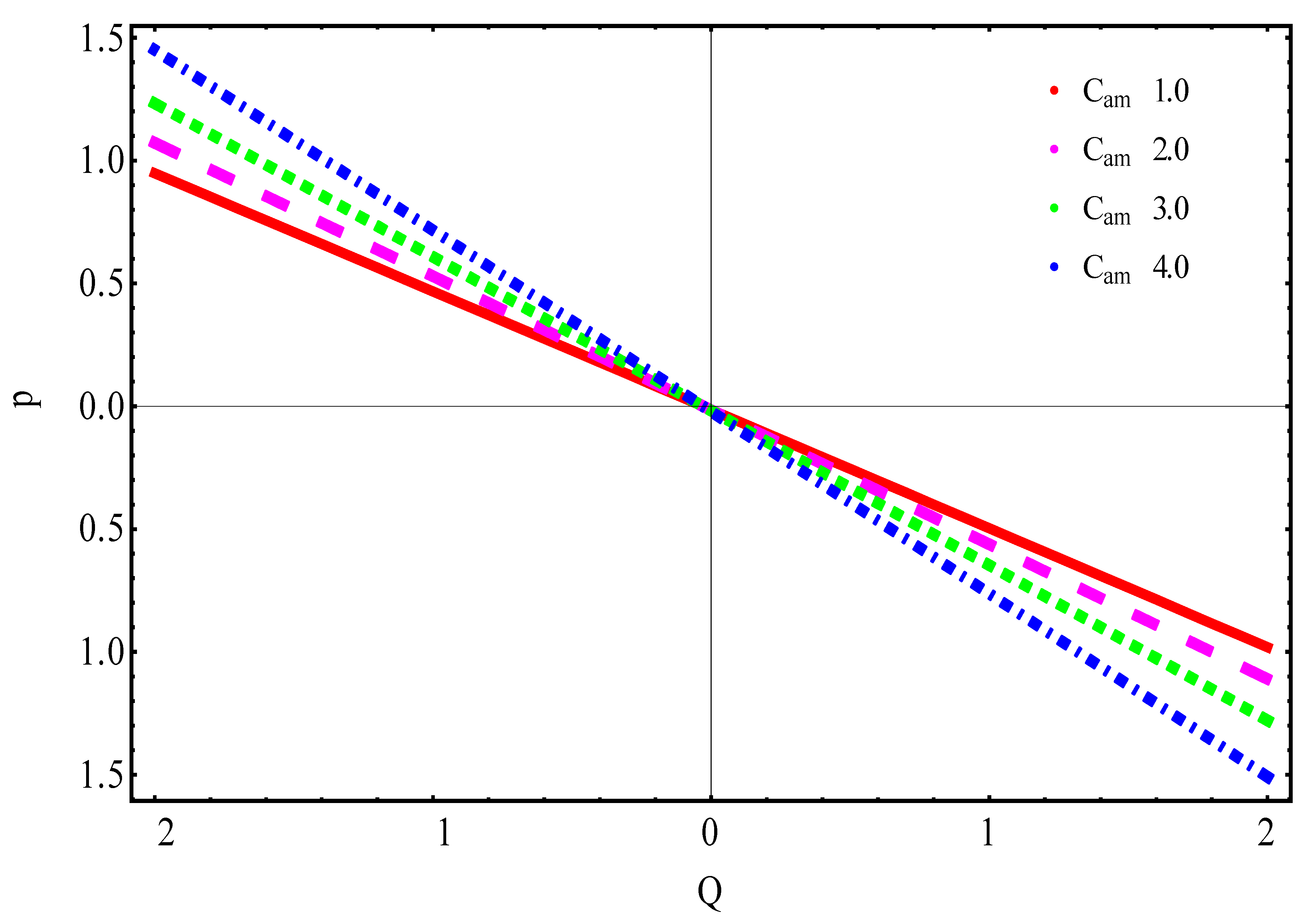
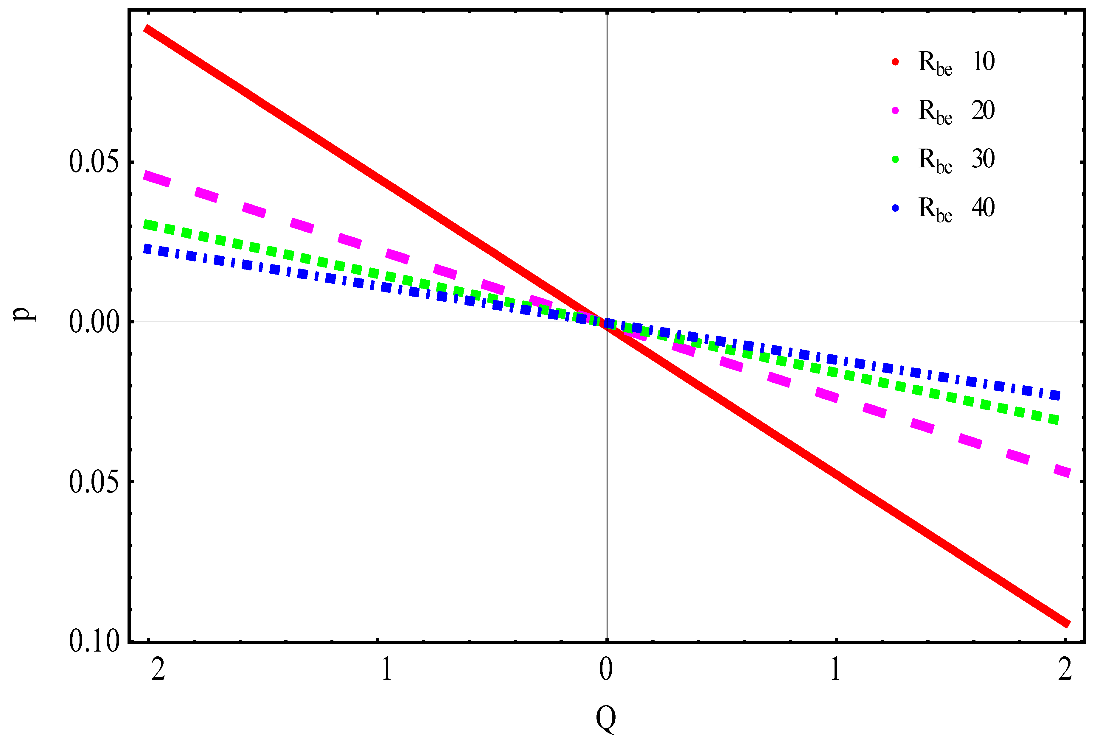
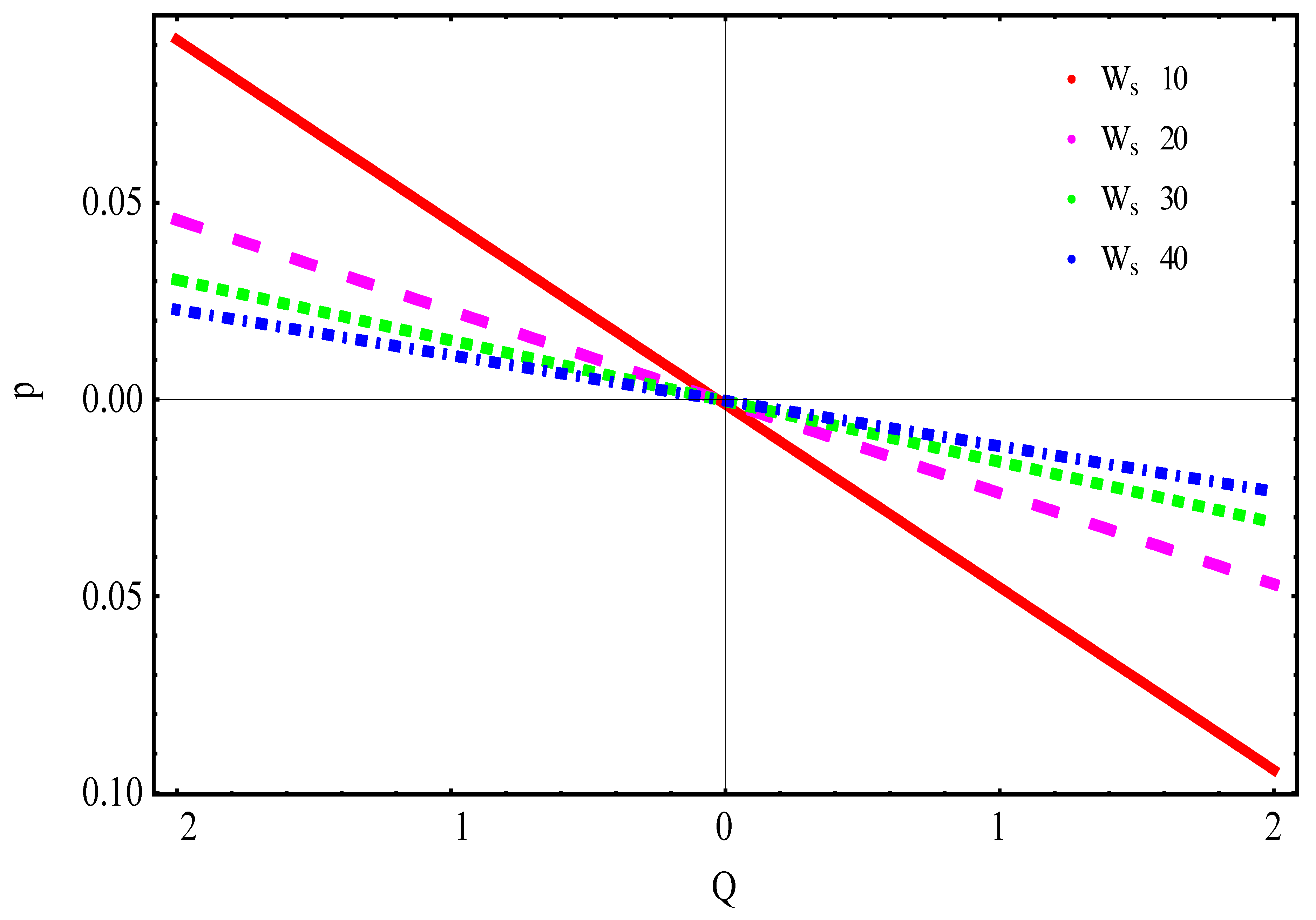
4.1. Pressure Rising

The flow of biological fluid in peristaltic motion circulating in the human body are investigated in Figure 2, Figure 3, Figure 4 and Figure 5. The pressure rise was defined as Δ P = 0 1 d x . In Figure 2, it can be seen that by increasing the value of the Eotvos number, the pumping rate rose in the co-pumping region ( Δ p < 0 ,   Q > 0 ) , whereas the opposite behavior was seen in the retrograde pumping region ( Δ p > 0 ,   Q < 0 ) , ( Δ p < 0 ,   Q < 0 ) and the free pumping region. From Figure 3 it is noticeable that the pumping rate dropped ( Δ p < 0 ,   Q > 0 ) in the co-pumping region when we increased the value of the added mass coefficient and the free pumping region ( Δ p < 0 ,   Q < 0 ) . In the retrograde pumping region ( Δ p > 0 ,   Q < 0 ) the opposite behavior was noted. It can be seen in Figure 4, that when we increased the value of Reynolds’ number R be , the pumping rate rose in the co-pumping region ( Δ p 0 ,   Q 0 ) . However, the behavior was the opposite in the retrograde pumping region ( Δ p > 0 ,   Q < 0 ) and in the free pumping region ( Δ p < 0 ,   Q < 0 ) . From Figure 5, it is noticeable that there was an upsurge in the pumping rate ( Δ p < 0 ,   Q > 0 ) in the co-pumping region by increasing values of slip velocity and free pumping region ( Δ p < 0 ,   Q < 0 ) . In the retrograde pumping region ( Δ p > 0 ,   Q < 0 ) the behavior was quite the opposite.

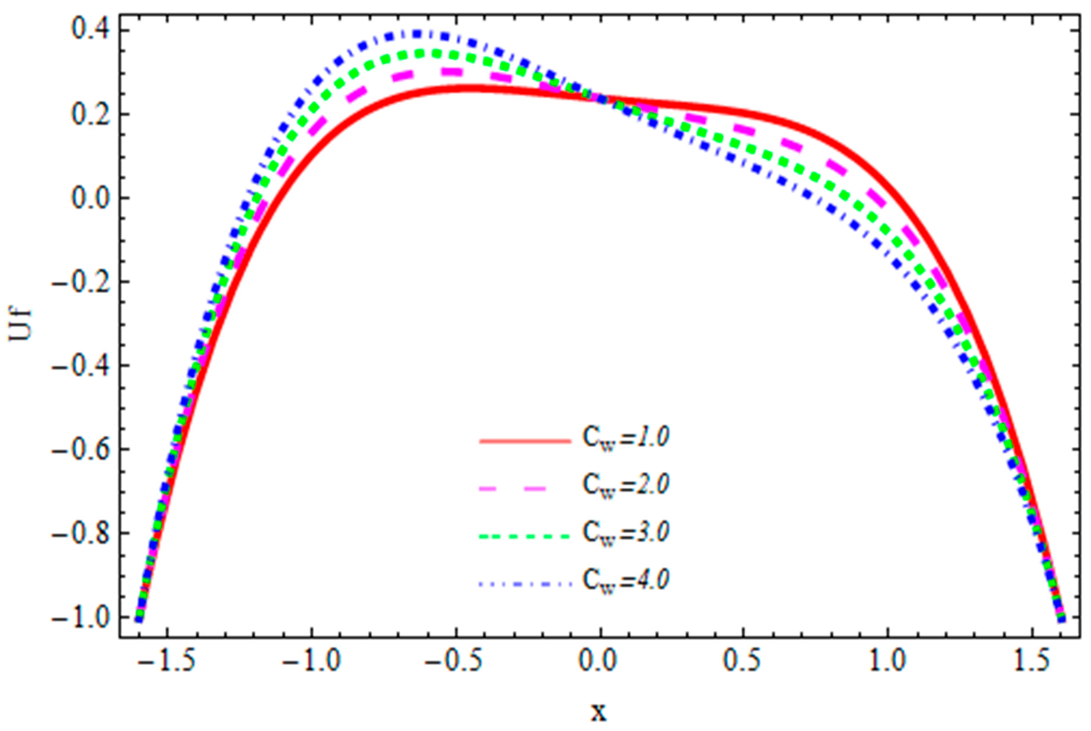
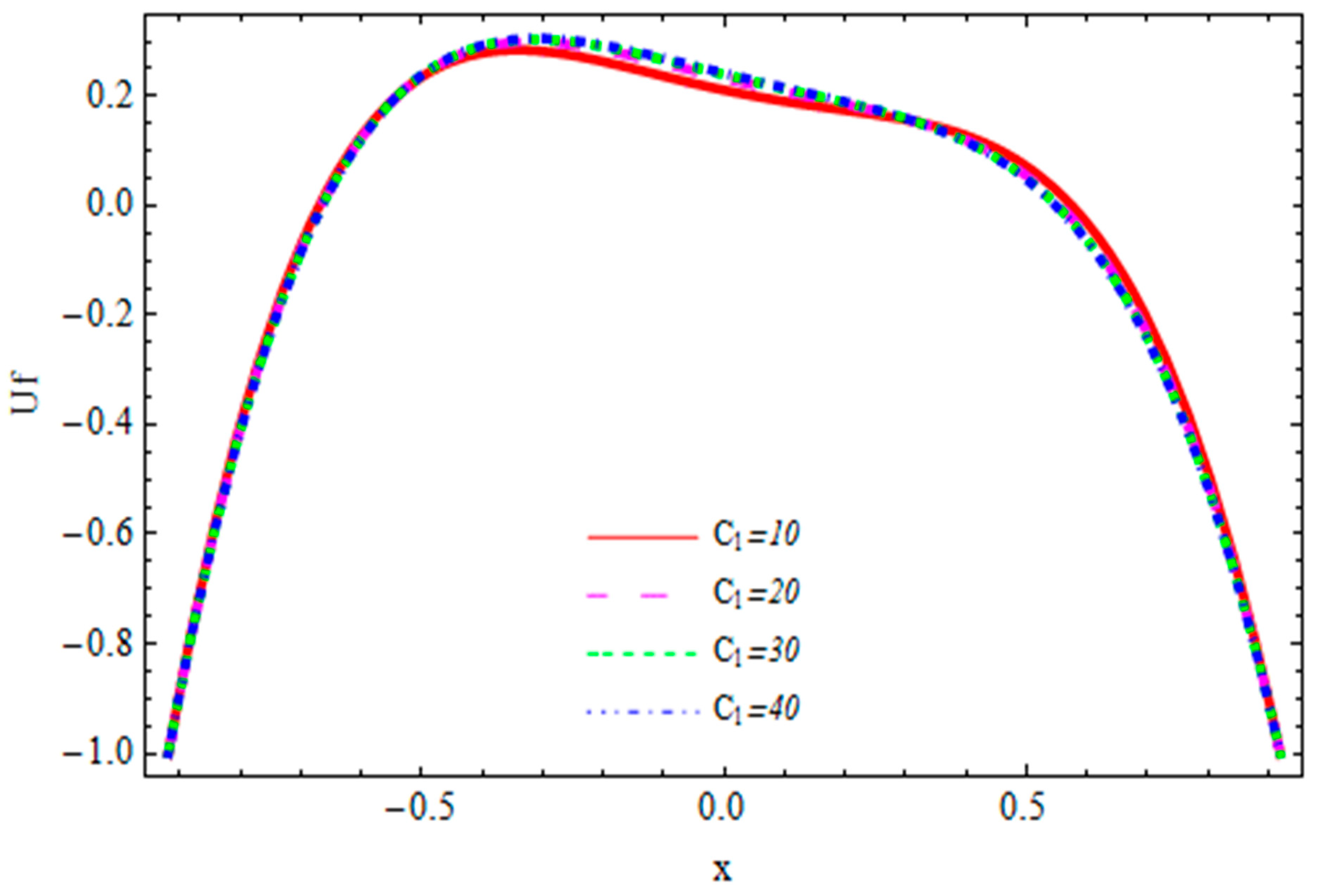
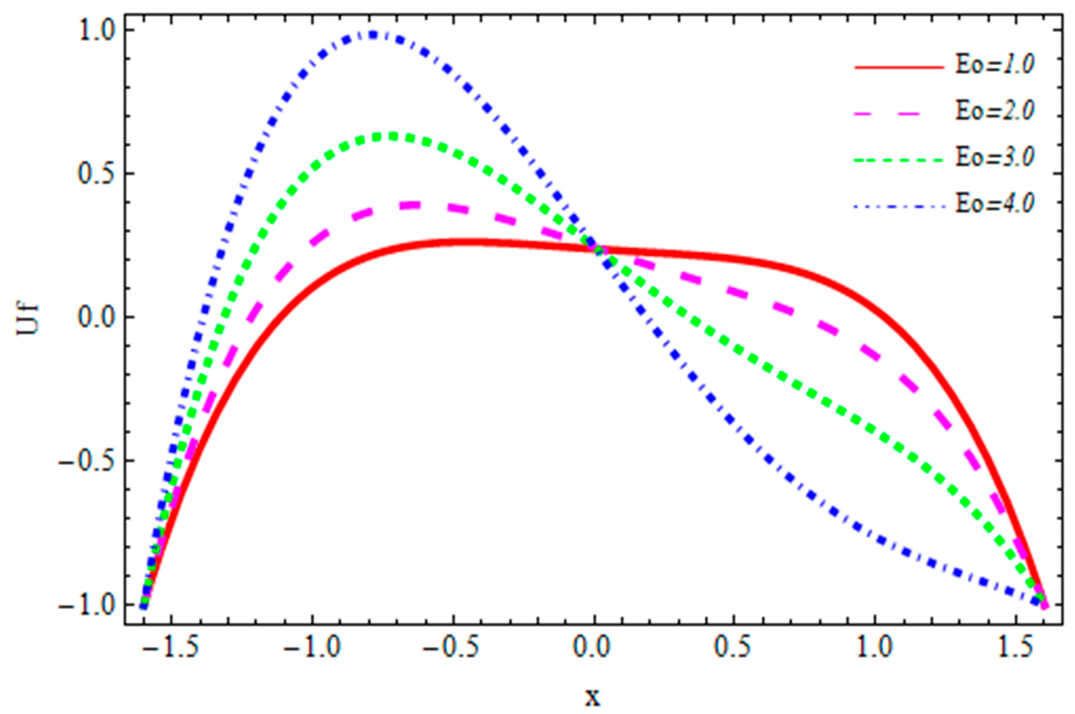
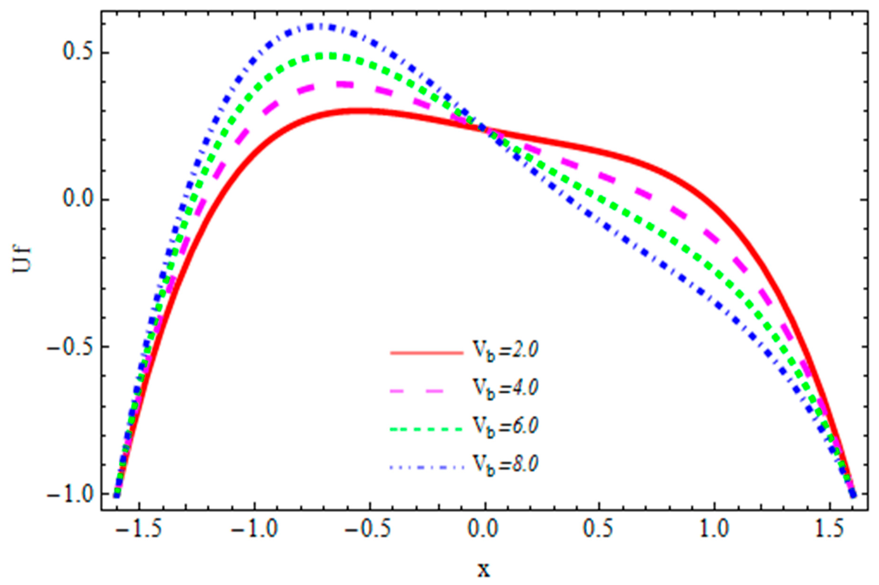
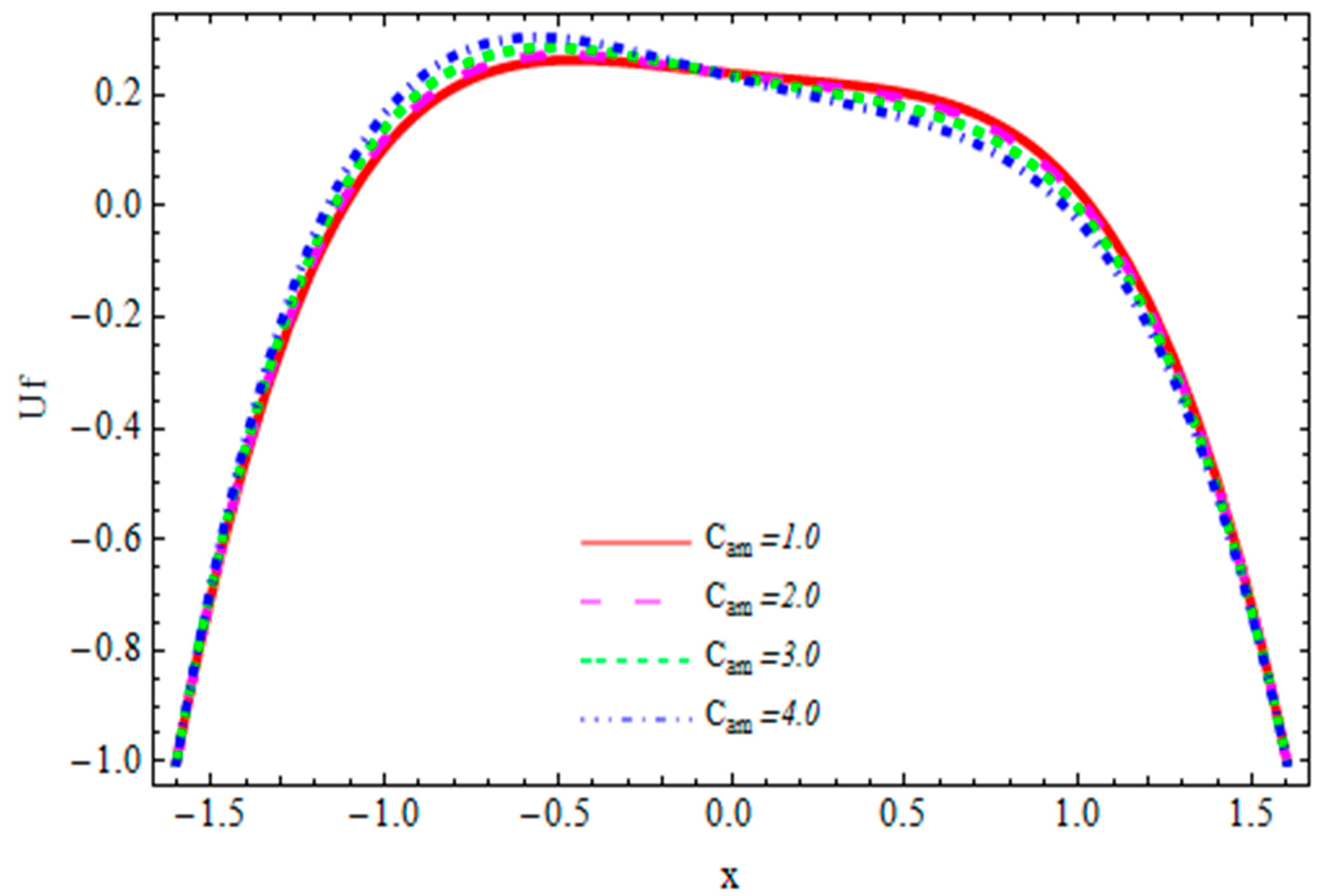
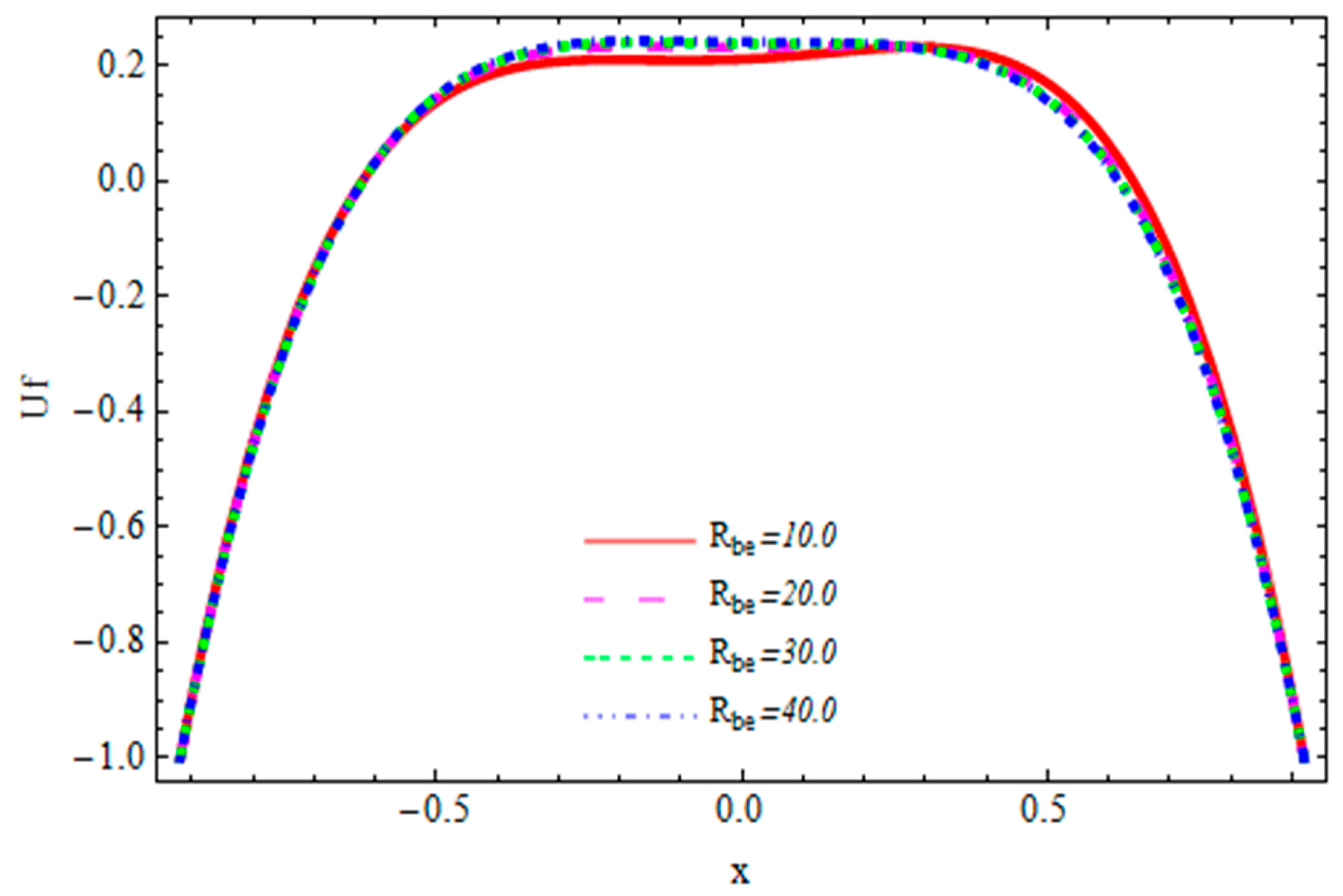
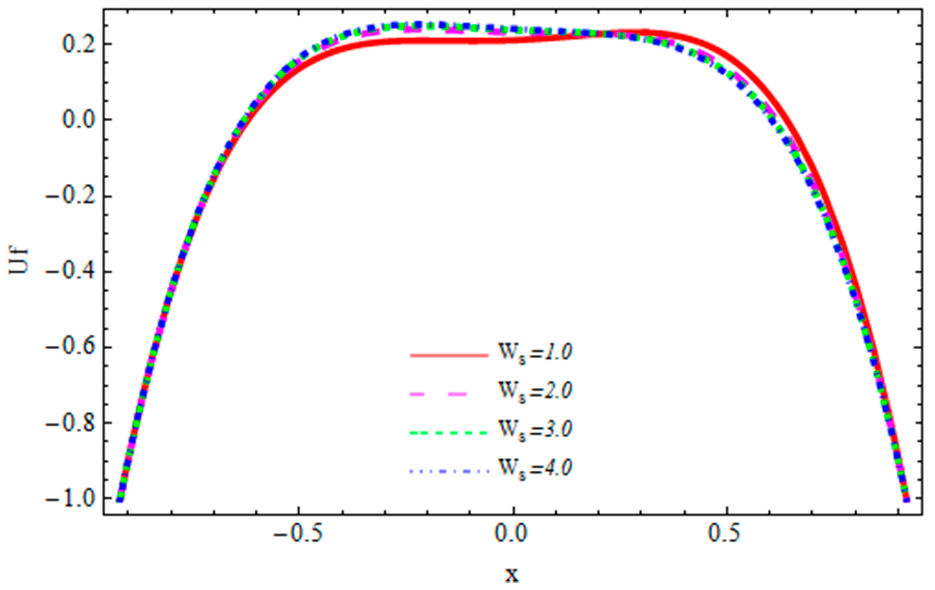
4.2. Fluid Velocity Profile

The fluid and gas velocities are examined in Figure 6, Figure 7, Figure 8, Figure 9, Figure 10, Figure 11, Figure 12, Figure 13, Figure 14, Figure 15, Figure 16, Figure 17, Figure 18 and Figure 19. The effect of the model coefficient on the flow velocity was increased when we increased the value of the model coefficient, as seen in Figure 6. It is clear from Figure 7 that with increasing values of the lift coefficient, there was an upturn in the velocity of fluid. From Figure 8, it is found that the behavior of the velocity reduced with the increasing values of the Eotvos number because the Eotvos number is the ratio of gravitation force to surface tension. The larger values of E o represented lesser surface tension and an increase in gravity resulted in the reduction of velocity. In Figure 9, we observed that when we increased the values of volume, the velocity reduced. Due to the rise in bubble volume, drag force increased and, hence, fluid slowed down. The fluid velocity decreased by increasing the value of the added mass coefficient as depicted in Figure 10. The added mass force increased with the rise in bubble volume because it was a drag force due to accelerating bubbles, hence the velocity of the fluid reduced. It is clear from Figure 11 that with rising values of R be the velocity of the fluid was decreased. R be was a parameter related to bubble volume directly, with a constant fluid density it behaved similar to V b . From Figure 12, it was detected that the behavior of velocity reduced with increasing values of the slip velocity.

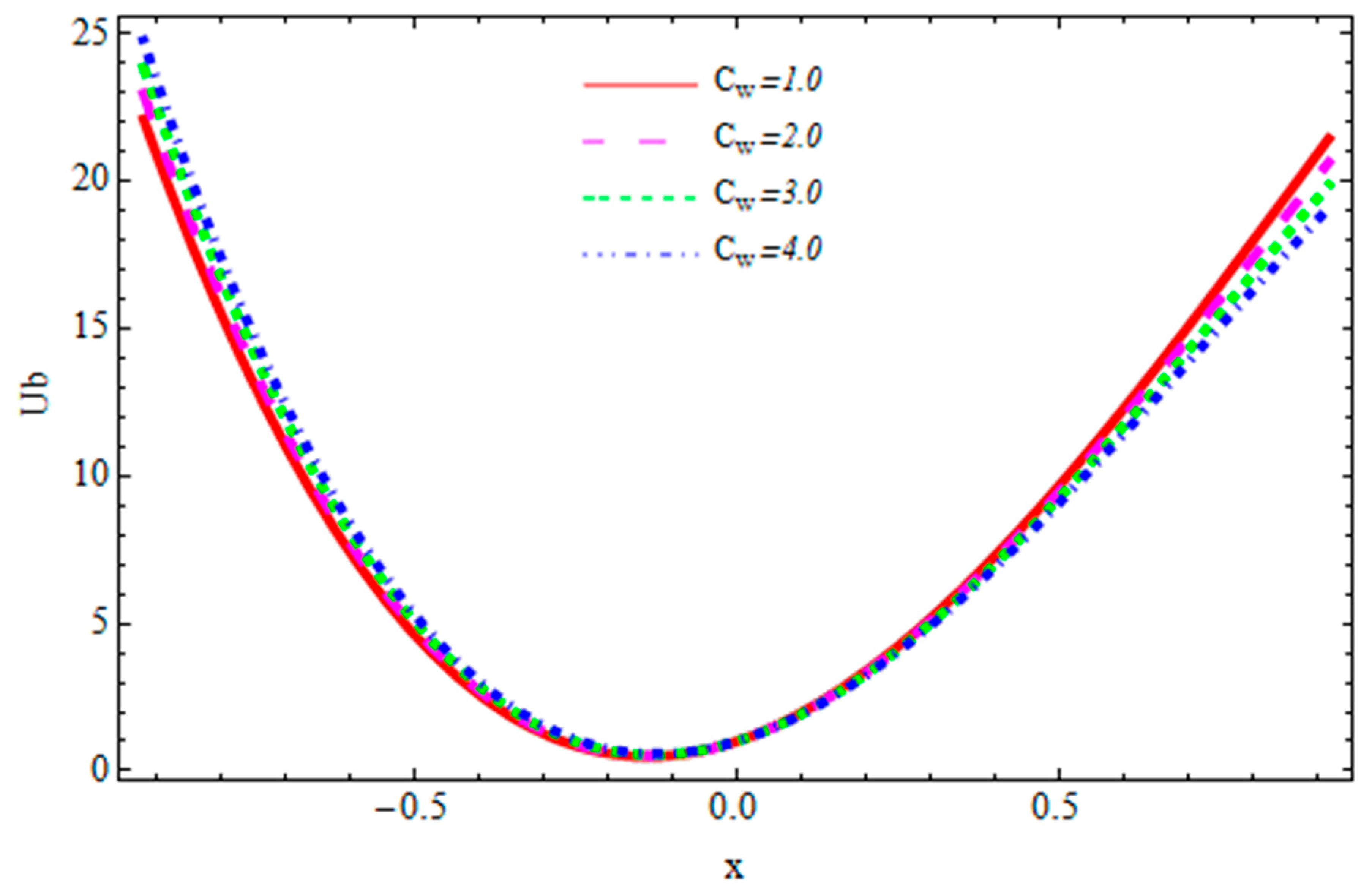
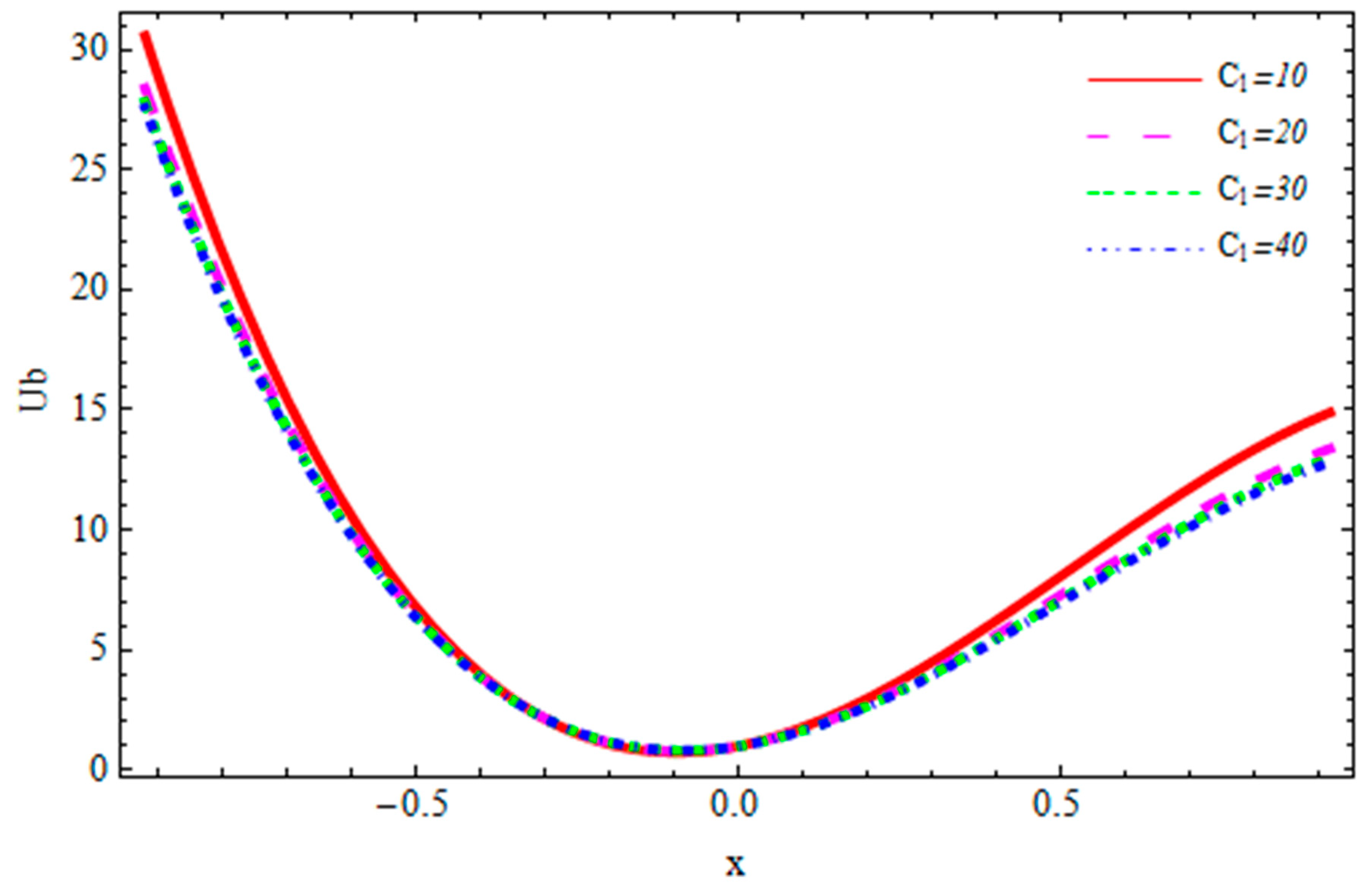
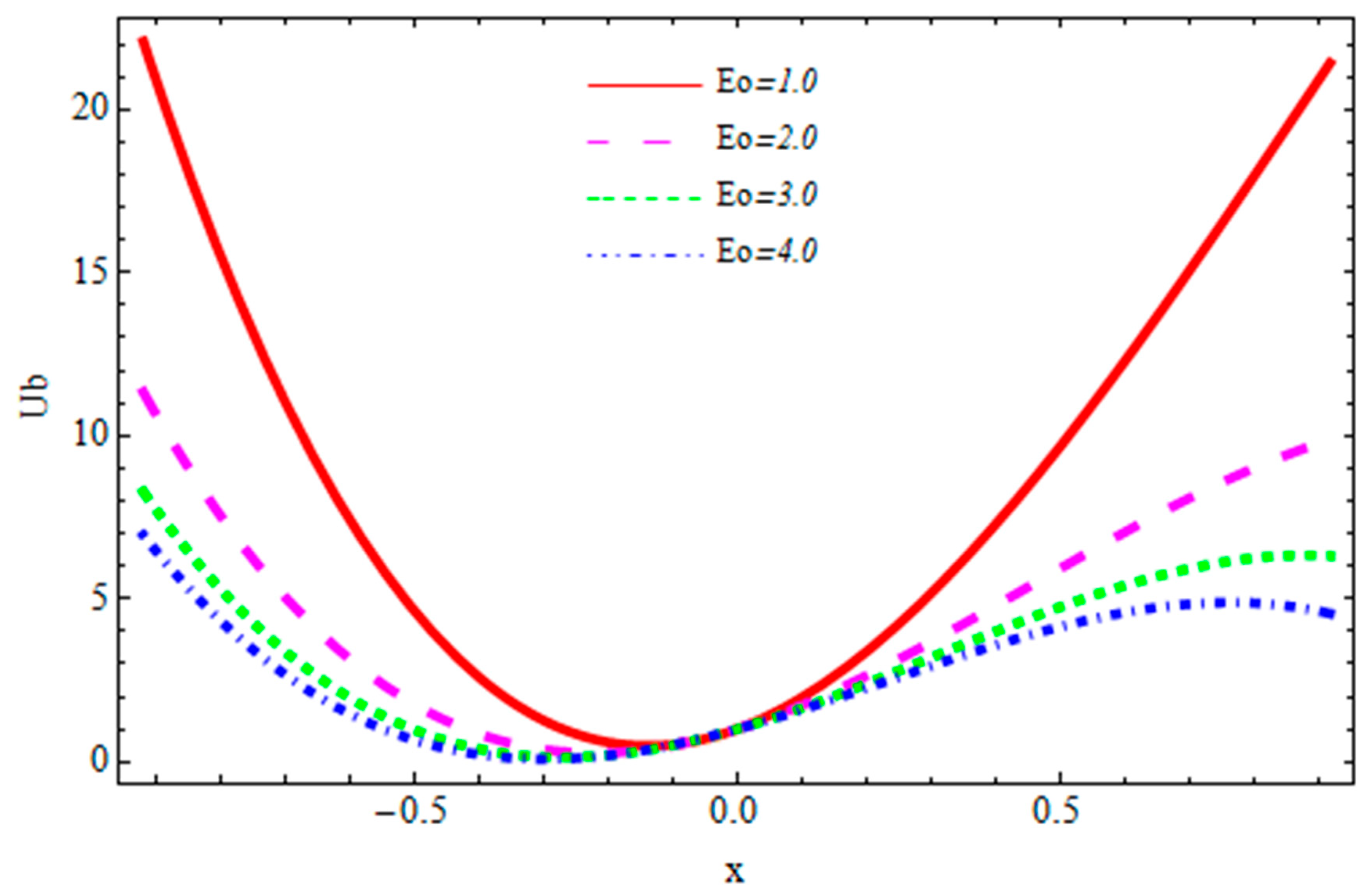
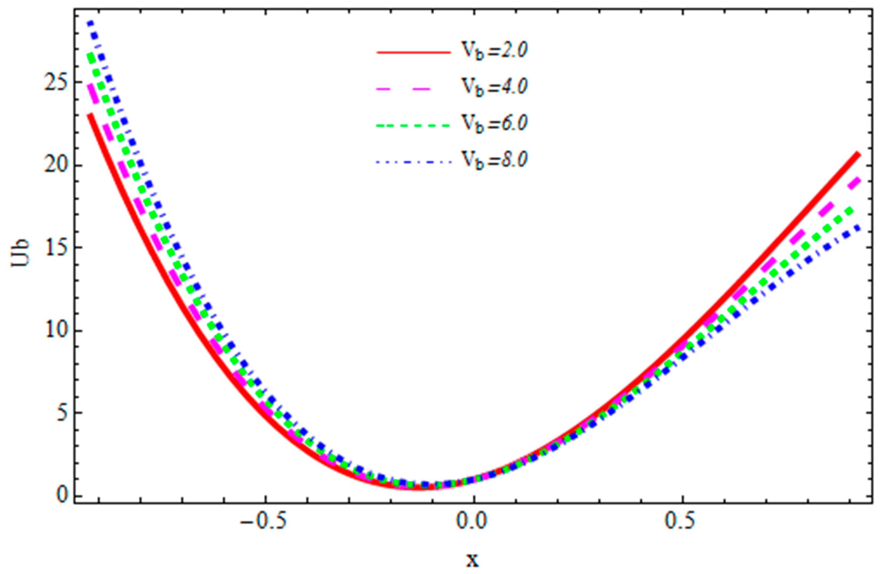
4.3. Gas Velocity Profile

The effect of the model coefficient on the flow velocity declined for higher values of the model coefficient, as displayed in Figure 13. It is clear in Figure 14 that with the increase of the lift coefficient, the velocity of fluid went up. From Figure 15, it was perceived that the behavior of the velocity rose with the increasing values of the Eotvos number. It can be perceived from Figure 16, that when we increased the values of volume, a dipping behavior of the velocity was grasped. The fluid velocity increased with increasing values of the added mass coefficient, as portrayed in Figure 17. From Figure 18, it can be concluded that with an increase in the values of R be , the velocity of fluid increases. Figure 19 shows that the velocity rose with the increasing values of the slip velocity.

5. Conclusions

In this investigation, the rheological properties of the liquid influenced the coating to make dynamical behavior nonlinear. Due to nonlinearity, first the constraints of low Reynolds number and long wavelength approximations, after transforming the actual frame into a wave frame, were used, and then the nonlinear coupled equations were solved by a well-known perturbation technique. The physical effects of prominent parameters, namely volume, Eotvos number, mass coefficient, slip velocity, and model coefficients were examined and discussed.

Author Contributions

Conceptualization, R.E.; investigation, N.I.; methodology, A.R.; validation, A.Z.; writing―review and editing, S.M.S. All authors have read and agreed to the published version of the manuscript.

Funding

This research received no external funding.

Conflicts of Interest

The authors declare no conflict of interest.

References

  1. Sussman, M.; Smereka, P.; Osher, S. A level set approach for computing solutions to incompressible two-phase flow. J. Comput. Phys. 1994, 114, 146–159. [Google Scholar] [CrossRef]
  2. Bankoff, S.G. A variable density single-fluid model for two-phase flow with particular reference to steam-water flow. J. Heat Transfer 1960, 82, 265–270. [Google Scholar] [CrossRef]
  3. Zuber, N.; Findlay, J. Average volumetric concentration in two-phase flow systems. J. Heat Transfer 1965, 87, 453–468. [Google Scholar] [CrossRef]
  4. Picchi, D.; Poesio, P. A unified model to predict flow pattern transitions in horizontal and slightly inclined two-phase gas/shear-thinning fluid pipe flows. Int. J. Multiphase Flow 2016, 84, 279–291. [Google Scholar] [CrossRef]
  5. Sato, Y.; Sekoguchi, K. Liquid velocity distribution in two-phase bubble flow. Int. J. Multiphase Flow 1975, 2, 79–95. [Google Scholar] [CrossRef]
  6. Kuwagi, K.; Ozoe, H. Three-dimensional oscillation of bubbly flow in a vertical cylinder. Int. J. Multiphase Flow 1999, 25, 175–182. [Google Scholar] [CrossRef]
  7. Picchi, D.; Battiato, I. The impact of pore-scale flow regimes on upscaling of immiscible two-phase flow in porous media. Water Resources Res. 2018, 54, 6683–6707. [Google Scholar] [CrossRef]
  8. Bonzanini, A.; Picchi, D.; Ferrari, M.; Poesio, P. Shape factors inclusion in a one-dimensional, transient two-fluid model for stratified and slug flow simulations in pipes. In Proceedings of the 12th International Conference on Computational Fluid Dynamics in the Oil & Gas, Metallurgical and Process Industries, Trondheim, Norway, May/June 2017. [Google Scholar]
  9. Sontti, S.G.; Atta, A. Numerical investigation of viscous effect on Taylor bubble formation in co-flow microchannel. Comp. Aided Chem. Eng. 2017, 40, 1201–1206. [Google Scholar]
  10. Bhatti, M.M.; Zeeshan, A.; Ellahi, R.; Shit, G.C. Mathematical modeling of heat and mass transfer effects on MHD peristaltic propulsion of two-phase flow through a Darcy-Brinkman-Forchheimer porous medium. Adv. Powder Technol. 2018, 29, 1189–1197. [Google Scholar] [CrossRef]
  11. Haider, S.; Ijaz, N.; Zeeshan, A.; Li, Y.Z. Magneto-hydrodynamics of a solid-liquid two-phase fluid in rotating channel due to peristaltic wavy movement. Int. J. Numer. Methods Heat Fluid Flow 2019. [Google Scholar] [CrossRef]
  12. Depner, T.A.; Rizwan, S.Y.E.D.; Stasi, T.A. Pressure effects on roller pump blood flow during hemodialysis. ASAIO Trans. 1990, 36, M456-9. [Google Scholar]
  13. Haight, L.G.; Herbst, R.; Winterton, R.F.; Sorenson, J.L. Patent and Trademark Office. US Patent No. 6,234,992, 2001. [Google Scholar]
  14. Tripathi, D.; Sharma, A.; Bég, O.A. Joule heating and buoyancy effects in electro-osmotic peristaltic transport of aqueous nanofluids through a microchannel with complex wave propagation. Adv. Powder Technol. 2018, 29, 639–653. [Google Scholar] [CrossRef]
  15. Animasaun, I.L.; Pop, I. Numerical exploration of a non-Newtonian Carreau fluid flow driven by catalytic surface reactions on an upper horizontal surface of a paraboloid of revolution, buoyancy and stretching at the free stream. Alexandria Eng. J. 2017, 56, 647–658. [Google Scholar] [CrossRef]
  16. Angirasa, D.; Peterson, G.P.; Pop, I. Combined heat and mass transfer by natural convection with opposing buoyancy effects in a fluid saturated porous medium. Int. J. Heat Mass Transfer 1997, 40, 2755–2773. [Google Scholar] [CrossRef]
  17. Rashidi, M.M.; Rostami, B.; Freidoonimehr, N.; Abbasbandy, S. Free convective heat and mass transfer for MHD fluid flow over a permeable vertical stretching sheet in the presence of the radiation and buoyancy effects. Ain Shams Eng. J. 2014, 5, 901–912. [Google Scholar] [CrossRef]
  18. Masud, U.; Baig, M.I.; Zeeshan, A. Automatization analysis of the extremely sensitive laser-based dual-mode biomedical sensor. Lasers Med. Sci. 2020. [CrossRef]
  19. Liu, S.; Yang, K.; Wang, Y.; Qu, J.; Liao, C.; He, J.; Li, Z.; Yin, G.; Sun, B.; Zhou, J.; et al. High-sensitivity strin sensor based on in-fiber rectangular air bubble. Scientif. Rep. 2015, 5, 7624. [Google Scholar] [CrossRef] [Green Version]
  20. Guo, W.; Liu, J.; Liu, J.; Wang, G.; Wang, G.; Huang, M. A Single-Ended Ultra-Thin Spherical Microbubble Based on the Improved Critical-State Pressure-Assisted Arc Discharge Method. Coatings 2019, 9, 144. [Google Scholar] [CrossRef] [Green Version]
  21. Ellahi, R.; Zeeshan, A.; Hussain, F.; Safaei, M.R. Simulation of cavitation of spherically shaped hydrogen bubbles through a tube nozzle with stenosis. Int. J. Numerical Methods Heat Fluid Flow 2020. [Google Scholar] [CrossRef]
  22. Prakash, J.; Tripathi, D.; Tiwari, A.K.; Sait, S.M.; Ellahi, R. Peristaltic pumping of nanofluids through a tapered channel in a porous environment: Applications in blood flow. Symmetry 2019, 11, 868. [Google Scholar] [CrossRef] [Green Version]
  23. Hussain, F.; Ellahi, R.; Zeeshan, A.; Vafai, K. Modelling study on heated couple stress fluid peristaltically conveying gold nanoparticles through coaxial tubes: A remedy for gland tumors and arthritis. J. Mol. Liq. 2018, 268, 149–155. [Google Scholar] [CrossRef]
  24. Zeeshan, A.; Ijaz, N.; Majeed, A. Analysis of magnetohydrodynamics peristaltic transport of hydrogen bubble in water. Int. J. Hydrogen Energy 2018, 43, 979–985. [Google Scholar] [CrossRef]
  25. Drew, D.A.; Lahey, R.T., Jr. Application of general constitutive principles to the derivation of multidimensional two-phase flow equations. Int. J. Multiphase Flow 1979, 5, 243–264. [Google Scholar] [CrossRef]
  26. Maskaniyan, M.; Nazari, M.; Rashidi, S.; Mahian, O. Natural convection and entropy generation analysis inside a channel with a porous plate mounted as a cooling system. Thermal Sci. Eng. Progr. 2018, 6, 186–193. [Google Scholar] [CrossRef]
  27. Zeeshan, A.; Hussain, F.; Ellahi, R.; Vafai, K. A study of gravitational and magnetic effects on coupled stress bi-phase liquid suspended with crystal and Hafnium particles down in steep channel. J. Mol. Liq. 2019, 286, 110898. [Google Scholar] [CrossRef]
  28. Picchi, D.; Poesio, P. Stability of multiple solutions in inclined gas/shear-thinning fluid stratified pipe flow. Int. J. Multiphase Flow 2016, 84, 176–187. [Google Scholar] [CrossRef]
  29. Picchi, D.; Barmak, I.; Ullmann, A.; Brauner, N. Stability of stratified two-phase channel flows of Newtonian/non-Newtonian shear-thinning fluids. Int. J. Multiphase Flow 2018, 99, 111–131. [Google Scholar] [CrossRef] [Green Version]
  30. Suckale, J.; Qin, Z.; Picchi, D.; Keller, T.; Battiato, I. Bi-stability of buoyancy-driven exchange flows in vertical tubes. J. Fluid Mech. 2018, 850, 525–550. [Google Scholar] [CrossRef] [Green Version]
  31. De Bertodano, M.L.; Lahey, R.T., Jr.; Jones, O.C. Phase distribution in bubbly two-phase flow in vertical ducts. Int. J. Multiphase Flow 1994, 20, 805–818. [Google Scholar] [CrossRef]
  32. Tyagi, P.; Buwa, V.V. Experimental characterization of dense gas–liquid flow in a bubble column using voidage probes. Chem. Eng. J. 2017, 308, 912–928. [Google Scholar] [CrossRef]
  33. Hu, D.; Han, G.; Lungu, M.; Huang, Z.; Liao, Z.; Wang, J.; Yang, Y. Experimental investigation of bubble and particle motion behaviors in a gas-solid fluidized bed with side wall liquid spray. Adv. Powder Technol. 2017, 28, 2306–2316. [Google Scholar] [CrossRef]
  34. Sarafraz, M.M.; Shadloo, M.S.; Tian, Z.; Tlili, I.; Alkanhal, T.A.; Safaei, M.R.; Arjomandi, M. Convective bubbly flow of water in an annular pipe: role of total dissolved solids on heat transfer characteristics and bubble formation. Water 2019, 11, 1566. [Google Scholar] [CrossRef] [Green Version]
  35. Ellahi, R.; Zeeshan, A.; Hussain, F.; Abbas, T. Study of shiny film coating on multi-fluid flows of a rotating disk suspended with nano-sized silver and gold particles: A comparative analysis. Coatings 2018, 8, 422. [Google Scholar] [CrossRef] [Green Version]
  36. Khan, Z.; Ur Rasheed, H.; Alharbi, S.O.; Khan, I.; Abbas, T.; Chin, D.L.C. Manufacturing of double layer optical fiber coating using phan-thien-tanner fluid as coating material. Coatings 2019, 9, 147. [Google Scholar] [CrossRef] [Green Version]
  37. Riaz, A.; A Al-Olayan, H.; Zeeshan, A.; Razaq, A.; Bhatti, M.M. Mass transport with asymmetric peristaltic propulsion coated with synovial fluid. Coatings 2018, 8, 407. [Google Scholar] [CrossRef] [Green Version]
  38. Bahgat Radwan, A.; Abdullah, A.M.; Mohamed, A.; Al-Maadeed, M.A. New electrospun polystyrene/Al2O3 nanocomposite superhydrophobic coatings; synthesis, characterization, and application. Coatings 2018, 8, 65. [Google Scholar] [CrossRef] [Green Version]
  39. Benkreira, H.; Ikin, J.B. Dissolution and growth of entrained bubbles when dip coating in a gas under reduced pressure. Chem. Eng. Sci. 2010, 65, 5821–5829. [Google Scholar] [CrossRef]
  40. Ellahi, R.; Zeeshan, A.; Hussain, F.; Abbas, T. Thermally charged MHD bi-phase flow coatings with non-Newtonian nanofluid and hafnium particles along slippery walls. Coatings 2019, 9, 300. [Google Scholar] [CrossRef] [Green Version]
  41. Marin, M. A domain of influence theorem for microstretch elastic materials. Nonl. Analy: Real World Appl. 2010, 11, 3446–3452. [Google Scholar] [CrossRef]
  42. Abd-Elaziz, E.M.; Marin, M.; Othman, M.I. On the effect of Thomson and initial stress in a thermo-porous elastic solid under GN electromagnetic theory. Symmetry 2019, 11, 413. [Google Scholar] [CrossRef] [Green Version]
  43. Akram, S.; Mekheimer, K.S.; Elmaboud, Y.A. Particulate suspension slip flow induced by peristaltic waves in a rectangular duct: effect of lateral walls. Alexandria Eng. J. 2018, 57, 407–414. [Google Scholar] [CrossRef] [Green Version]
  44. Ishii, M.; Hibiki, T. Thermo-Fluid Dynamics of Two-Phase Flow; Springer: New York, NY, USA, 2010. [Google Scholar]
  45. Sokolichin, A.; Eigenberger, G.; Lapin, A. Simulation of buoyancy driven bubbly flow: established simplifications and open questions. AIChE J. 2004, 50, 24–45. [Google Scholar] [CrossRef]
  46. Drew, D.A. Mathematical modeling of two-phase flow. Ann. Rev. Fluid Mech. 1983, 15, 261–291. [Google Scholar] [CrossRef]
  47. Auton, T.R. The lift force on a spherical body in a rotational flow. J. Fluid Mech. 1987, 183, 199–218. [Google Scholar] [CrossRef]
  48. He, J.H. Linearized perturbation technique and its applications to strongly nonlinear oscillators. Comp. Math. Appl. 2003, 45, 1–8. [Google Scholar] [CrossRef] [Green Version]
  49. He, J.H. A note on the homotopy perturbation method. Thermal Sci. 2010, 14, 565–568. [Google Scholar]
  50. Dehghan, M.; Rahmani, Y.; Ganji, D.D.; Saedodin, S.; Valipour, M.S.; Rashidi, S. Convection–radiation heat transfer in solar heat exchangers filled with a porous medium: homotopy perturbation method versus numerical analysis. Renew. Energy 2015, 74, 448–455. [Google Scholar] [CrossRef]
  51. Ungarish, M. Hydrodynamics of Suspensions: Fundamentals of Centrifugal and Gravity Separation; Springer: New York, NY, USA, 2013. [Google Scholar]
Figure 1. Geometry of the problem.
Coatings 10 00115 g001
Figure 2. Pressure rise for several values of E o .
Coatings 10 00115 g002
Figure 3. Pressure rise for several values of C a m .
Coatings 10 00115 g003
Figure 4. Pressure rise for several values of R be .
Coatings 10 00115 g004
Figure 5. Pressure rise for several values of W s .
Coatings 10 00115 g005
Figure 6. Fluid velocity curves for several values of C w . R be = 10 ,   V b = 1.0 ,   E o = 1.0 ,   C a m = 1.0 ,     W s = 10 ,   C l = 10 .
Coatings 10 00115 g006
Figure 7. Fluid velocity curves for several values of C l . R be = 10 ,   V b = 1.0 ,   E o = 1.0 ,   C a m = 1.0 ,     W s = 10 ,   C w = 10 .
Coatings 10 00115 g007
Figure 8. Fluid velocity curves for several values of E o . R be = 10 , V b = 1.0 ,   C l = 10 ,   C a m = 1.0 ,   W s = 10 ,   and   C w = 1.0 .
Coatings 10 00115 g008
Figure 9. Fluid velocity curves for several values of V b . R be = 10 ,   E o = 1.0 ,   C l = 10 ,   C a m = 1.0 ,   W s = 10 ,   and   C w = 1.0 .
Coatings 10 00115 g009
Figure 10. Fluid velocity curves for several values of C a m . R be = 10 ,   E o = 1.0 , C l = 10 , V b = 1.0 , W s = 10 ,   and   C w = 1.0 .
Coatings 10 00115 g010
Figure 11. Fluid velocity curves for several values of R be . C a m = 1.0 ,   E o = 1.0 ,   C l = 10 , V b = 1.0 , W s = 10 ,   and   C w = 1.0 .
Coatings 10 00115 g011
Figure 12. Fluid velocity curves for several values of W s . C a m = 1.0 ,   E o = 1.0 ,   C l = 10 ,   V b = 1.0 ,   R be = 10 ,   and   C w = 1.0 .
Coatings 10 00115 g012
Figure 13. Bubble velocity curves for several values of C w . R be = 10 ,   V b = 1.0 ,   E o = 1.0 , C a m = 1.0 ,   W s = 10 ,   and   C l = 10 .
Coatings 10 00115 g013
Figure 14. Bubble velocity curves for several values of C l . R be = 10 ,   V b = 1.0 ,   E o = 1.0 ,   C a m = 1.0 ,   W s = 10 ,   and   C w = 1.0 .
Coatings 10 00115 g014
Figure 15. Bubble velocity curves for several values of E o .     R be = 10 ,   V b = 1.0 ,   C l = 10 ,   C a m = 1.0 ,   W s = 10 ,   and   C w = 1.0 .
Coatings 10 00115 g015
Figure 16. Bubble velocity curves for several values of V b . R be = 10 ,   E o = 1.0 ,   C l = 10 ,   C a m = 1.0 ,   W s = 10 ,   and   C w = 1.0 .
Coatings 10 00115 g016
Figure 17. Bubble velocity curves for several values of C a m . R be = 10 ,   E o = 1.0 , C l = 10 ,   V b = 1.0 ,   W s = 10 ,   and   C w = 1.0 .
Coatings 10 00115 g017
Figure 18. Bubble velocity curves for several values of R be .   C a m = 1.0 ,   E o = 1.0 , C l = 10 ,   V b = 1.0 ,   W s = 10 ,   and   C w = 1.0 .
Coatings 10 00115 g018
Figure 19. Bubble velocity curves for several values of W s . R be = 10 , V b = 1.0 ,   E o = 1.0 , C a m = 1.0 ,   C w = 10 ,   and   C l = 10 .
Coatings 10 00115 g019

