1. Introduction
Human activity recognition (HAR) has allowed for the implementation of distinct applications such as user identification [
1], health monitoring [
2], identifying the early stage of depression [
3], fall detection [
4], and more. Improving these applications requires ongoing methodological development. Researchers have conducted many studies to improve HAR by introducing the recognition of various daily activities using divergent approaches that include non-identical machine learning algorithms. Improving HAR requires considering some inevitable challenges, which involve sensor orientation, sensor position, device independency, study sample length, and data volume [
5,
6,
7,
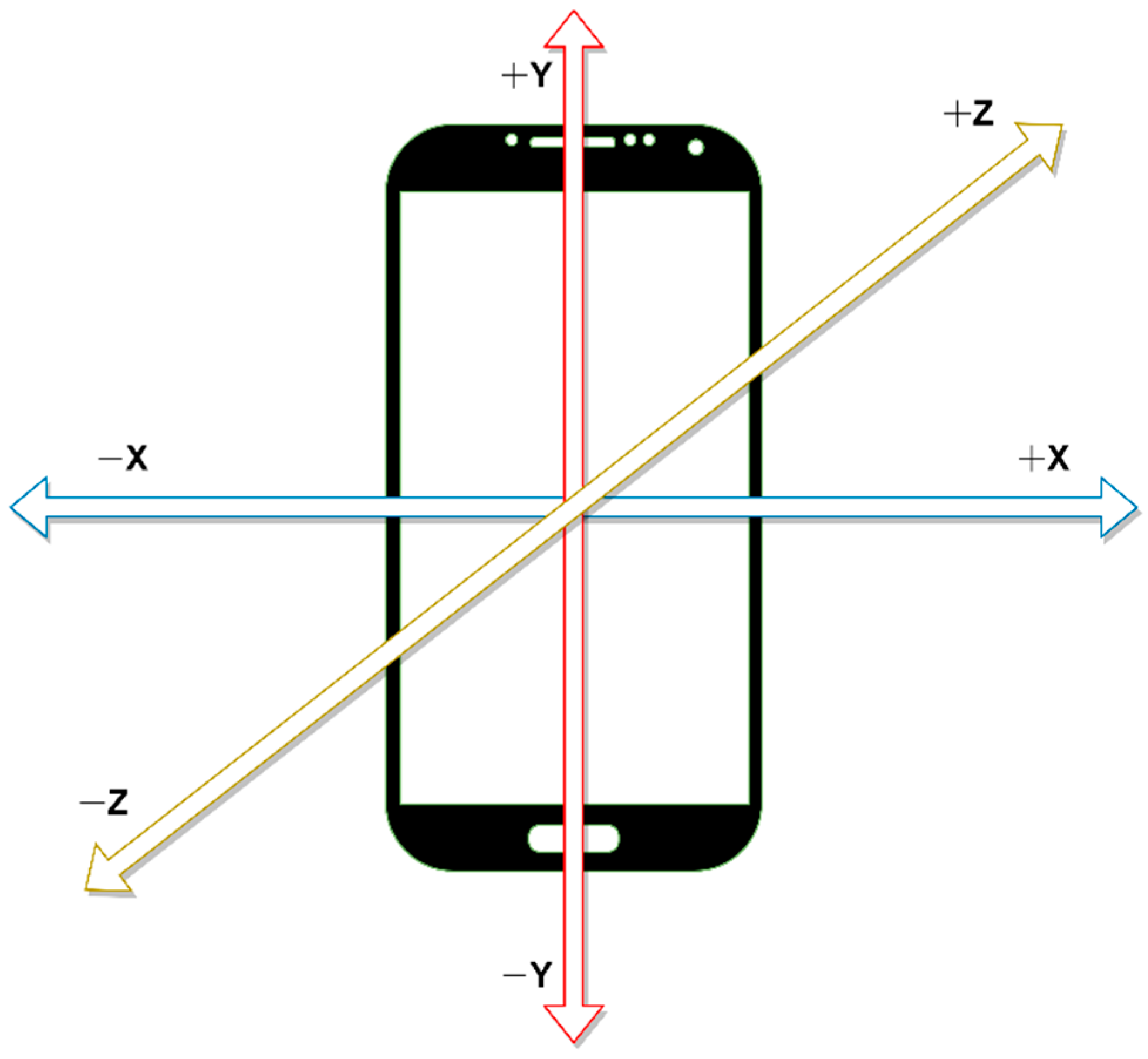
8]. Among the mentioned challenges, the most significant issue to solve is the problem of sensor orientation and position.
For solving the orientational and positional problem due to sensor placement, different studies have introduced techniques such as transforming the sensor signals to a universal frame, extracting orientation-invariant features from raw signals, removing orientation and position-specific information by introducing statistical alterations, estimating the orientation of the sensor to the earth frame by using the triaxial sensors (accelerometer, magnetometer, and gyroscope), and then transforming the raw signals from the sensor frame to the earth frame. Using the earth frame transformation approach [
9] achieved an average accuracy of 86.4% in recognizing 19 activities using support vector machine (SVM). The authors of [
10] introduced heuristic orientation invariant transformation and singular value decomposition-based transformation to tackle sensor orientation problems. They evaluated their approaches using 4 different classifiers on 5 distinct datasets. They found that their proposed approaches can reduce the accuracy drop by a considerable margin compared to other state-of-the-art approaches. The authors of [
11] decomposed the accelerometer signal into horizontal and vertical acceleration. They extracted nine features from the triaxial gyroscope sensor and horizontal and vertical acceleration signals to solve the position and orientation dependency problem. They acquired an accuracy of 91.27%, employing SVM to recognize 5 activities using the data from a smartphone in 4 different positions. For our study, we decided to utilize the features proposed by [
10] since it requires extracting nine simple features to eliminate the variation in data produced from sensor orientation and position. Along with the orientational and positional dependency obstacles, we should also consider the number of participants and activities appraised in former studies.
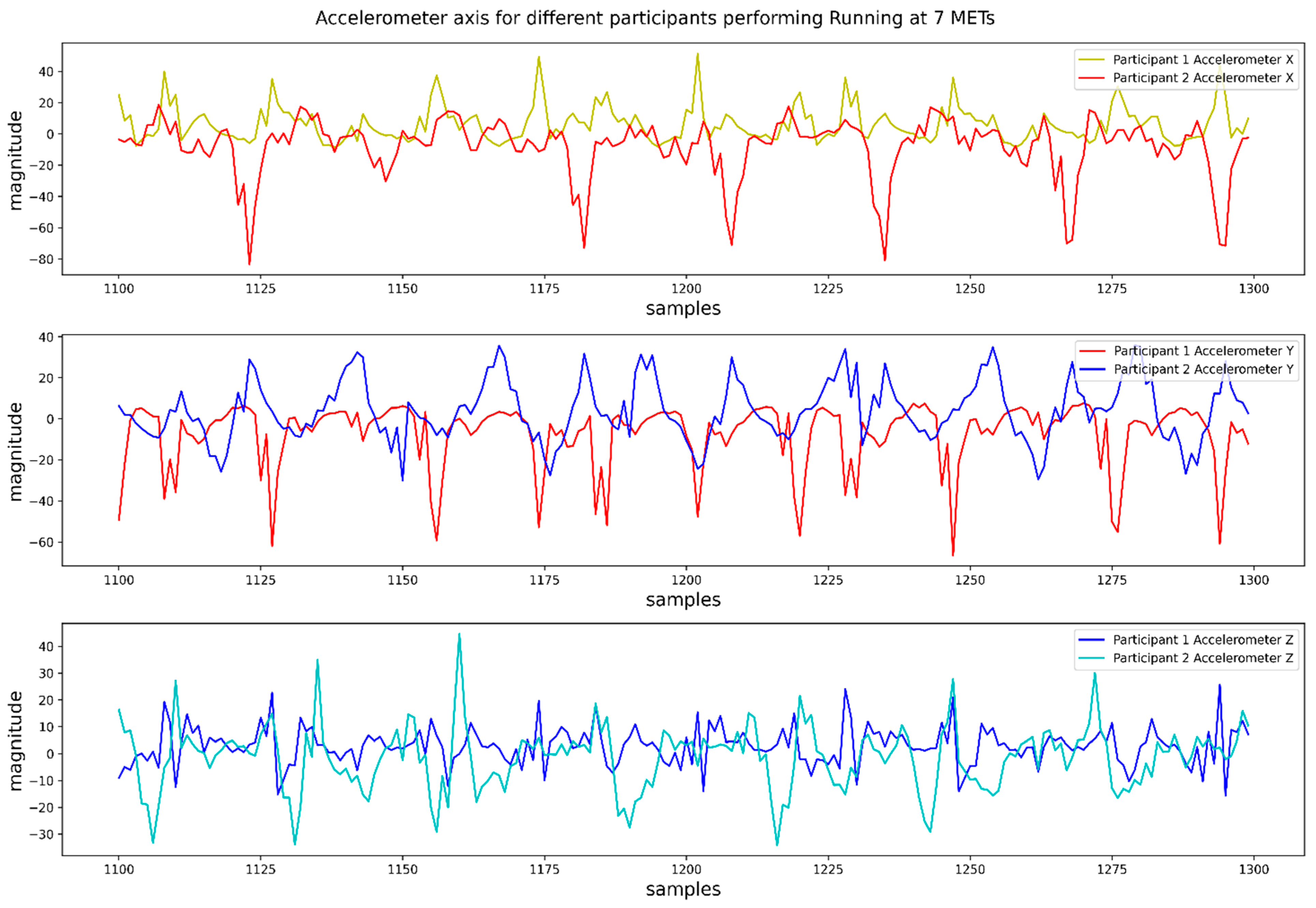
As the number of participants and activities varies, distinct variations in sensor signals appear due to the differences in the participants’ body attributes and the uniqueness in movements of the body parts during different activities. The number of participants matters, especially for the studies where the inter-participant evaluation technique is accepted as the validation method. There are many publicly available datasets to work with, and these have already been used in several studies that introduced different numbers of participants and activities [
12,
13,
14,
15,
16]. However, inter-participant evaluation for a large number of participants in the field of HAR is yet to be explored.
Regarding the employed classifiers for HAR, researchers evaluated the performance of both machine learning and deep learning algorithms. Research primarily assessed the performance of conventional machine learning algorithms such as support vector machine (SVM), decision tree, K-nearest neighbor, and random forest [
17,
18,
19,
20]. However, with the emergence of advanced computational power, deep learning algorithms became more common in HAR. The authors of [
12] evaluated the performance of the convolutional neural network (CNN), long short-term memory (LSTM), bidirectional-LSTM, and multilayer perceptron (MLP) using two public datasets named UCI [
21] and Pamap2 [
22]. They found that CNN outperformed other classifiers with 92.71% and 91% accuracy on UCI and Pamap2, respectively. The authors of [
23] compared CNN with state-of-the-art classifiers for classifying six activities and showed that CNN performed better than all other classifiers using features extracted by fast Fourier transform (FFT) with an accuracy of 95.75%. CNN remains favored for executing HAR because of its powerful ability to automatically extract features from raw signals using multiple filters [
24]. Studies then tried to combine the feature extraction power of CNN with LSTM’s power of persisting old information about time-series data. LSTM is an upgraded version of the recurrent neural network (RNN) that can preserve older information than RNN [
25]. The hybrid of CNN and LSTM, also called CNN-LSTM, has been used in different HAR studies. The authors of [
26] evaluated the performance of CNN-LSTM on HAR using three public datasets named UCI [
21], WISDM [
27], and OPPORTUNITY [
28]. They achieved accuracies of 95.78%, 95.85%, and 92.63% on UCI, WISDM, and OPPORTUNITY datasets, respectively, using a CNN-LSTM architecture. The authors of [
29] explored distinct deep learning architectures, including CNN-LSTM with their proposed margin-based loss function on OPPORTUNITY, UniMiB-SHAR [
15], and PAMAP2 datasets. The authors of [
30] ensembled three models, namely CNN-Net, Encoded-Net, CNN-LSTM, and found the performance of the ensembled model superior over six benchmark datasets.
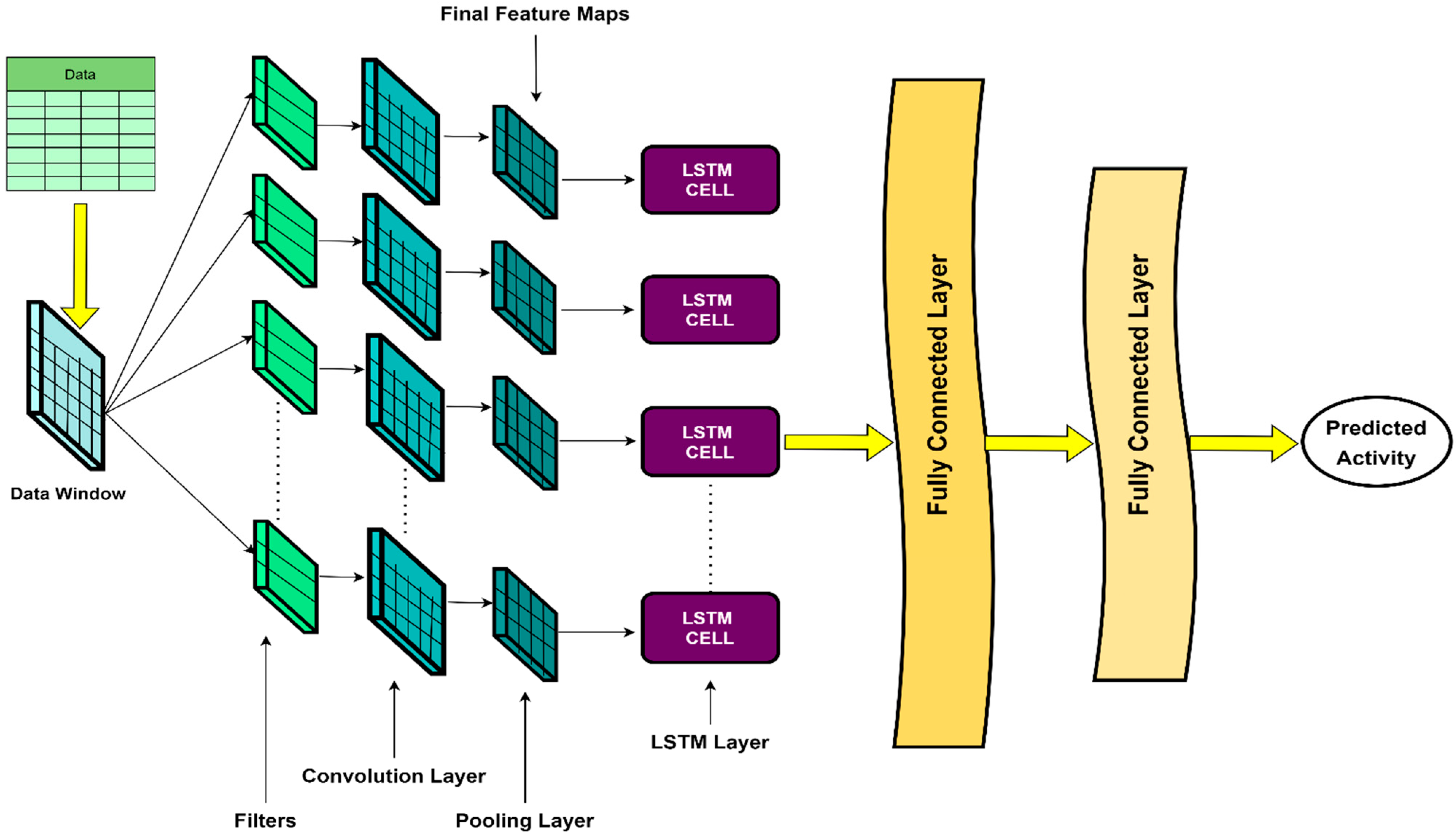
There are a number of different implementations of CNN for sensor data. Typically, 1-dimensional CNN (1D-CNN) is used for accelerometer, gyroscope, and magnetometer signals. An important consideration with 1D-CNN, LSTM, or their hybrid is that these methods require data windows as inputs. Each window resembles a data matrix with a fixed number of samples as rows and the features as columns. Each consecutive window may or may not overlap. 1D-CNN uses filters on each window to extract features automatically. 1D-CNN maps these internally extracted features to different activities in HAR research. However, when 1D-CNN is combined with LSTM, the internally extracted features from 1D-CNN work as inputs to the LSTM layers. These LSTM layers further process these automatically extracted features. The advantage of using a 1D-CNN-LSTM hybrid rather than using a single CNN or single LSTM is that 1D-CNN-LSTM can use the ability of CNN to extract spatial features present in the input data as well as preserve the temporal information present in the extracted spatial features using the ability of LSTM. Although a 1D-CNN-LSTM system takes more time in training than a single CNN, it should not impose any problem in the deployment of real-life applications since, in real life, pre-trained models are deployed. A detailed explanation of the working mechanism of 1D-CNN-LSTM will be given in a later section. Now that 1D-CNN works with windows of data, the length of windows can affect the performance of 1D-CNN. With a large window length, the model will have a bigger picture of the signals’ nature at a particular time. In contrast, a smaller window length portrays comparatively less information regarding the signal nature at any specific time. Again bigger windows increase the computational complexity and time complexity, whereas smaller windows keep the computational burden and processing time considerably lower. Previous studies selected the window length arbitrarily in HAR execution while using CNN, LSTM, or their hybridization, or they did not provide any discussion regarding the selection of window length [
23,
31,
32,
33,
34,
35]. It is yet to be explored how different window lengths may affect the performance of CNN, LSTM, or their hybrid models in HAR research.
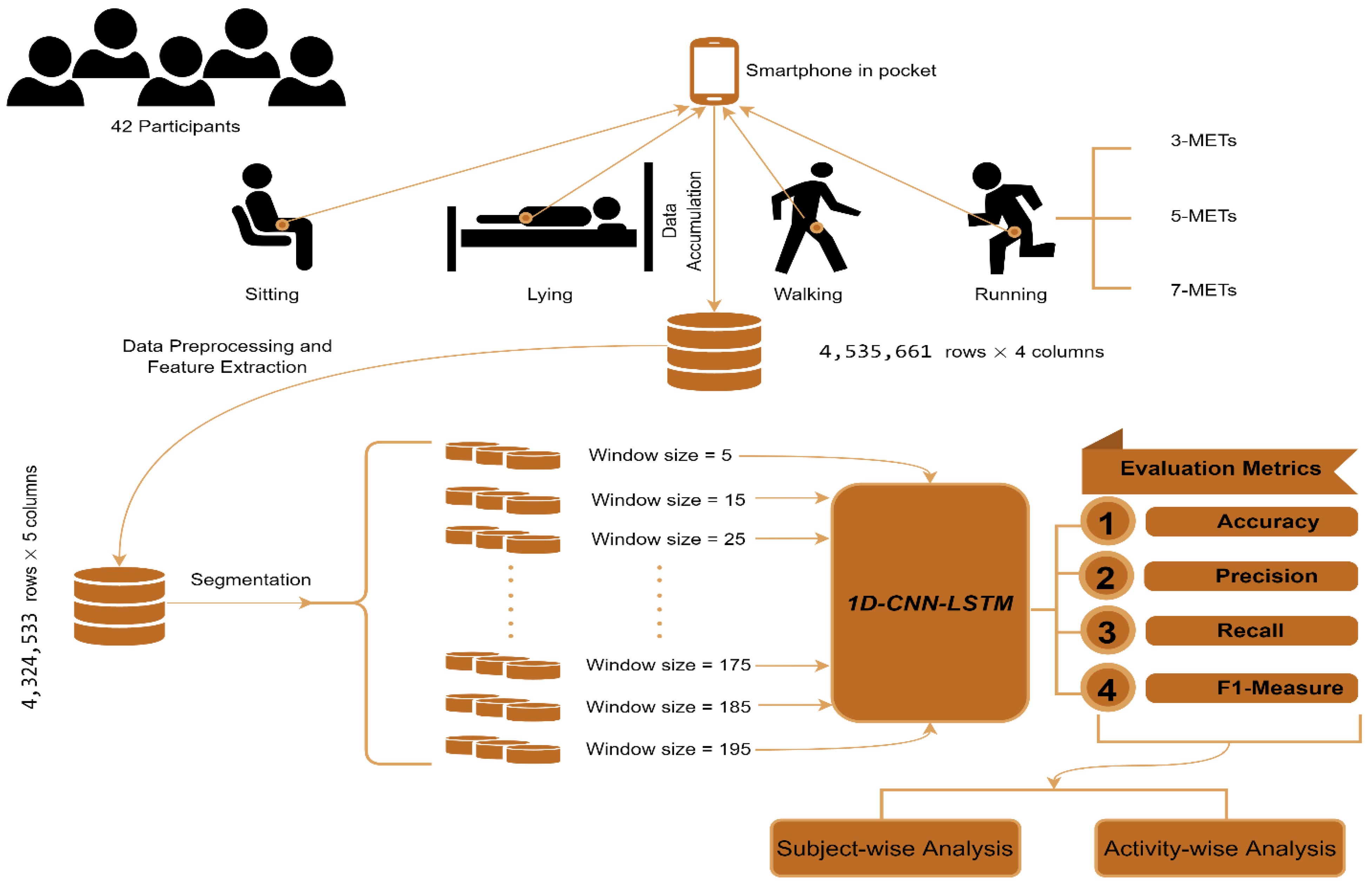
Considering the shortcomings mentioned above, the orientation problem, study sample lengths, and window length considerations, this paper systematically examines these limitations using feature extraction methods and window length experiments with 1D-CNN-LSTM models. A pictorial view of the overall procedure is portrayed in
Figure 1. Data from a study including 42 participants performing 6 activities, namely, sitting, lying, walking, and running at 3 metabolic equivalent tasks (METs), 5 METs, and 7 METs pace, were used. Data were collected using an accelerometer sensor of a smartphone carried by participants in their pockets. Specific research questions were:
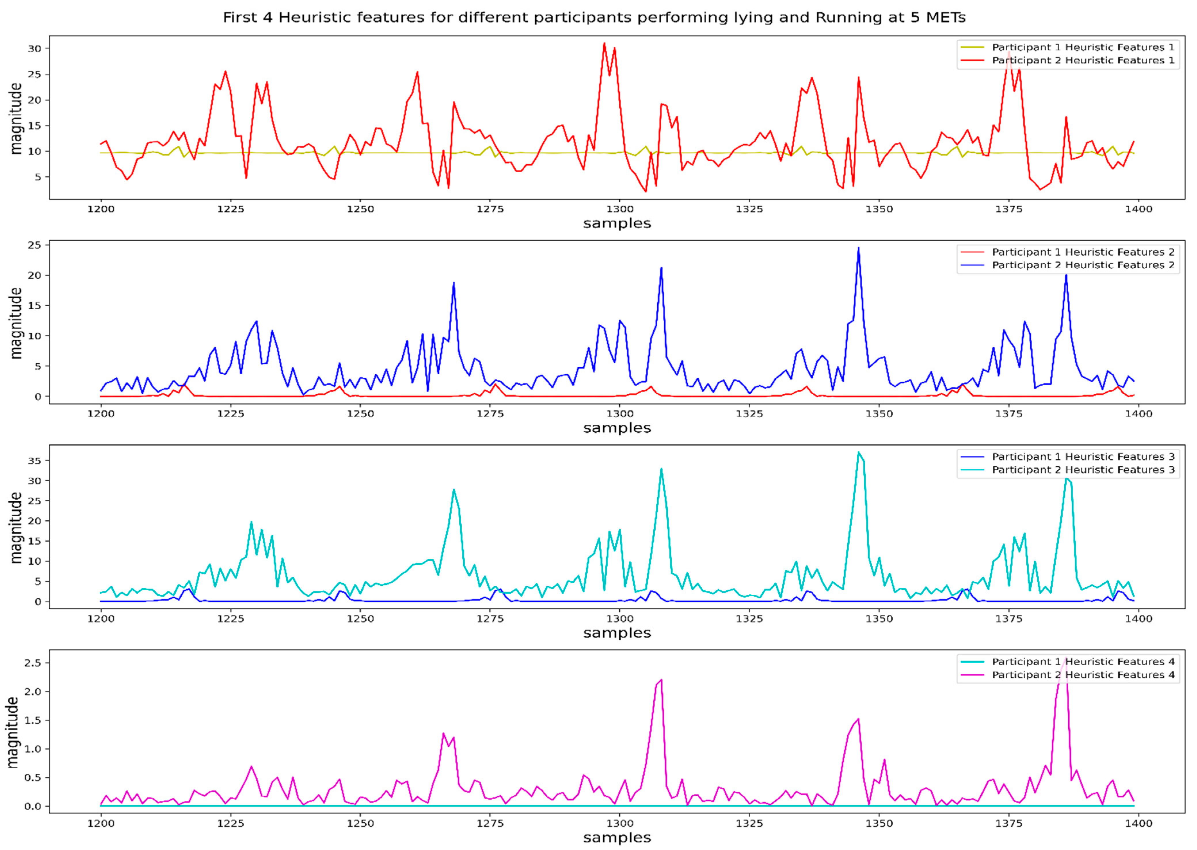
To solve the sensor orientation problem due to the flippable positions of the smartphone in the pocket, we selected 4 orientation-invariant heuristic features from the proposed 9 heuristic features in [
10].
Results show that after a particular window length, the performance of 1D-CNN-LSTM is not influenced by the window length. Further examination explores how different window lengths influence the recognition metrics for high- and low-intensity activities.
We found that the model did not produce the same performance when evaluated using data from different participants. Still, the effects of window length on the performance of the different participants were the same.
4. Discussion
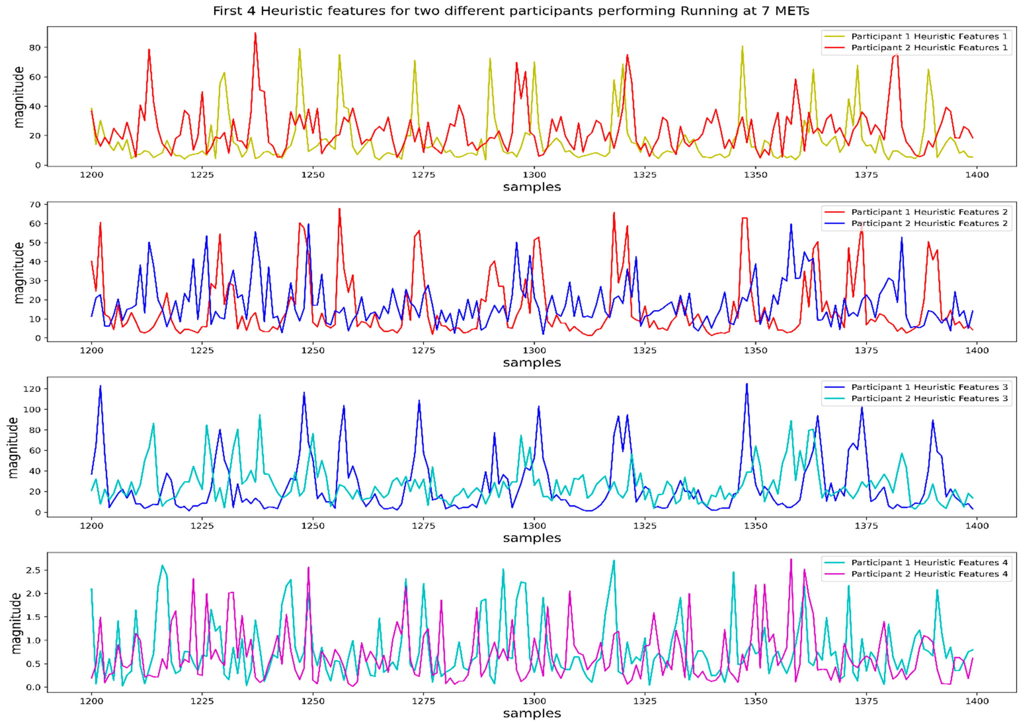
In [
10], researchers studied the performance of heuristic features for five publicly available datasets, which they labeled as A [
44], B [
45], C [
21], D [
46], and E [
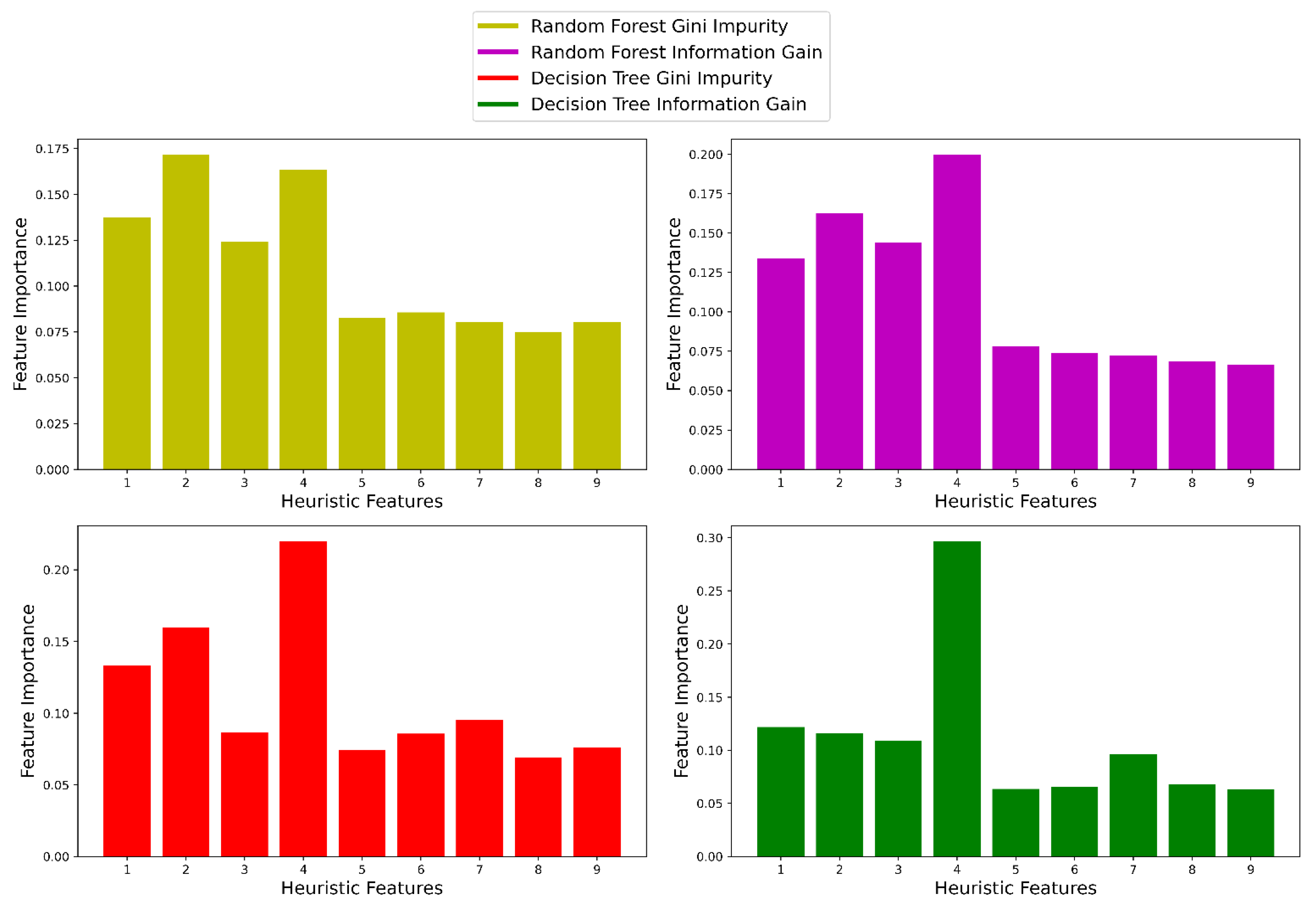
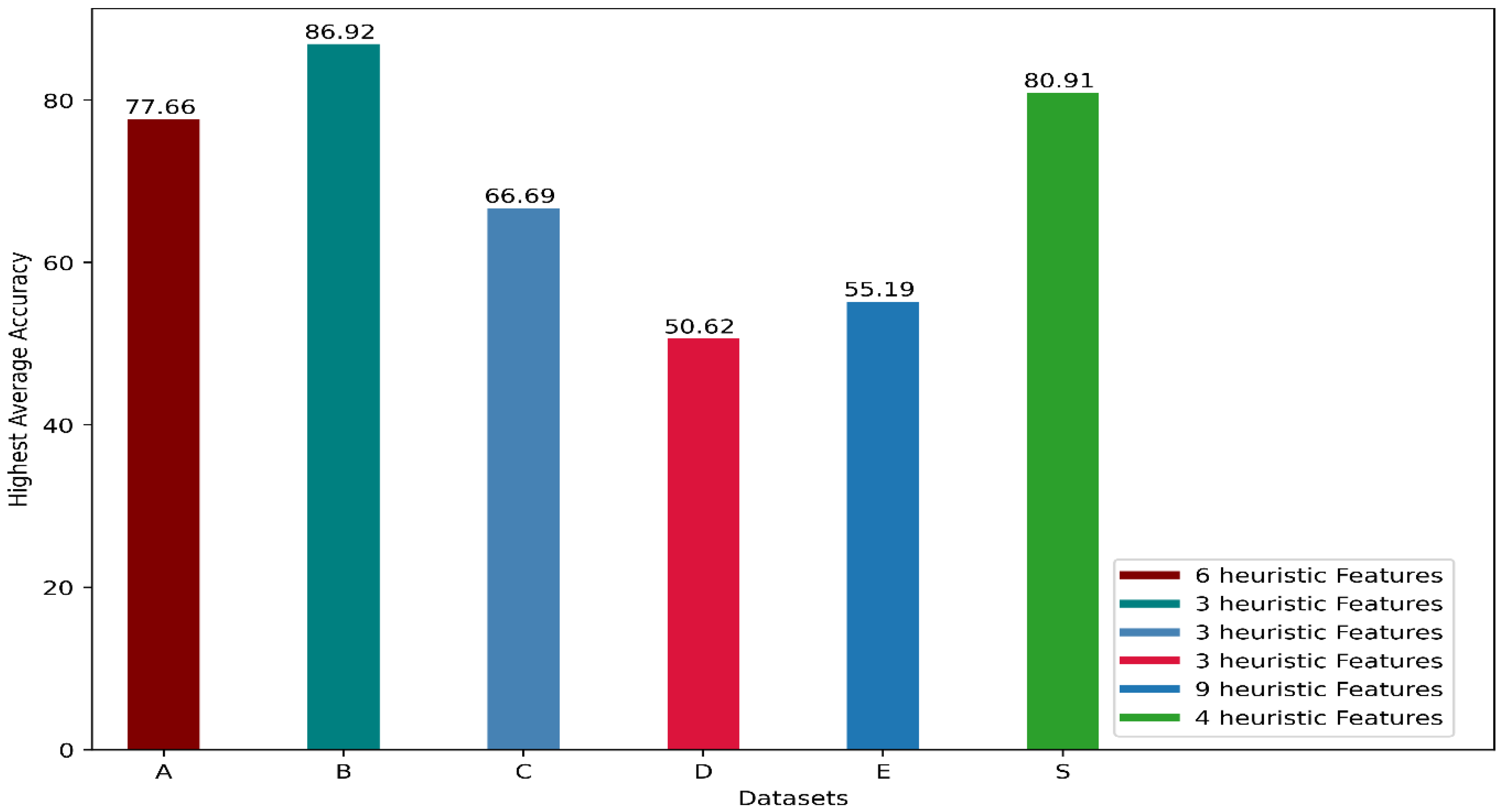
47]. Besides using the 9 features altogether, they also used only the first 3 or the first 6 heuristic features and recorded the performance of 4 classifiers, Bayesian decision-making (BDM), K-nearest neighbor (KNN), support vector machine (SVM), and artificial neural network (ANN). They used 10-fold cross-validation technique where each fold contained data for a particular participant. We can call our used inter-participant validation technique a 42-fold cross-validation technique where each fold contains data for a particular participant. They recorded accuracy from each classifier using the first 3 heuristic features, the first 6 heuristic features, and all 9 heuristic features. They achieved the highest accuracy for datasets B, C, and D using the first three heuristic features. To acquire the highest accuracy for datasets A and E, they used the first 6 and all 9 heuristic features, respectively. For all the datasets, they found the best performance using SVM. From their results, it was clear that all 9 heuristic features were not critically important to model performance since, for 3 of their datasets, they recorded the best performance using only the first 3 heuristic features. However, they did not try all the combinations of features, and there was no analysis to select the most significant features. We performed that analysis and found the first four features to be the most important. We plotted the highest accuracy they achieved using the heuristic features for each dataset and also indicated the number of features for which they found the best performance in
Figure 11. We also included the highest average accuracy we achieved, using the four most important features we found in the plot to provide a comparative perspective.
Although it is not feasible to compare our result with the results found in [
10] since they used different classifiers and datasets, we acquired results comparable to their performance, even with more participants than they had for an inter-participant validation method. However, our main objective was to explore the effects of window length in HAR execution for 1D-CNN-LSTM.
Many studies have explored HAR using deep neural networks like CNN, LSTM, or hybrids, but few studies in HAR have reported the effects of window length or time steps. Most of the studies chose the time steps or window length, claiming that they achieved the best performance using that particular window length. For instance, [
48] used a CNN and gated recurrent unit (GRU) hybrid on three datasets named UCI-HAR, WISDM, PAMAP2, and acquired 96.20%, 97.21%, 95.27%, respectively. Still, they did not mention how they chose the window length of 128 for their model. In another study [
49], which used the same dataset as in [
48], they also did not mention the reason behind choosing 128 as their window lengths; rather, they emphasized their proposed CNN, bidirectional LSTM hybrid-model architecture and acquired accuracies. Many other studies [
13,
50,
51,
52] explored divergent forms of deep learning architectures using the popular UCI-HAR dataset and used the same window length of 128 samples. Another study [
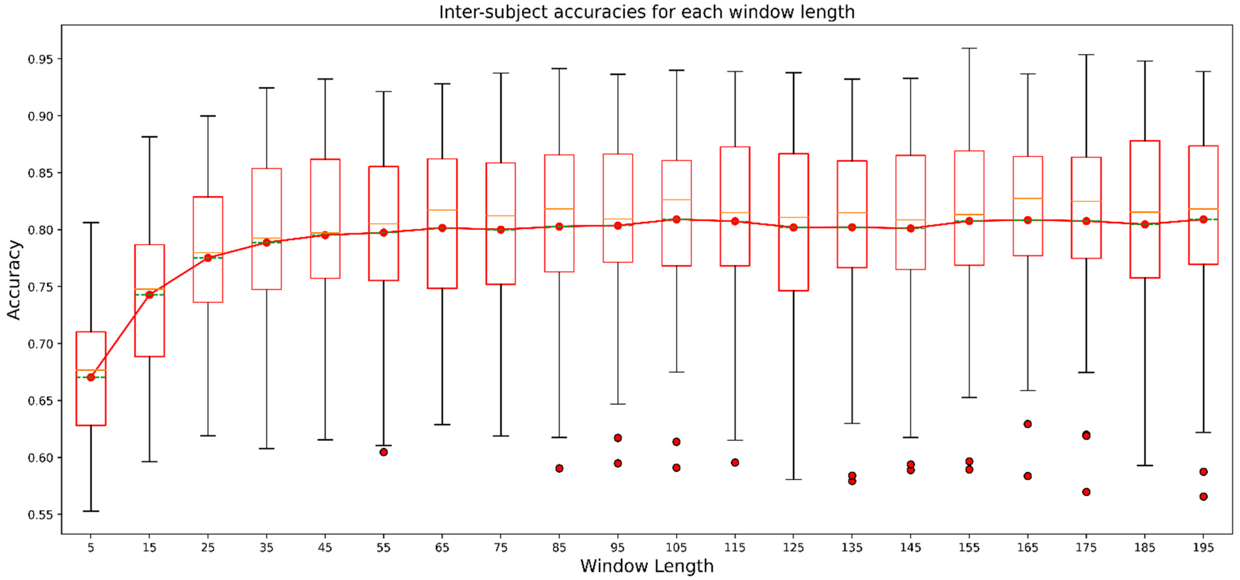
53], using a dataset called “Complex human activities using smartphones and smartwatch sensors”, explored the performance of divergent deep neural networks including LSTM, bidirectional LSTM, GRU, bidirectional GRU, CNN-LSTM, CNN-BiLSTM, CNN-GRU, and CNN-BiGRU for five different window lengths (in seconds) of 5, 10, 20, 30, and 40 s. They achieved the highest accuracy of 98.78% using CNN-BiGRU when they used the window length of 40 s. However, exploring only five different window lengths was insufficient to depict the influence of window lengths. Therefore in our study, we explored the performance of 1D-CNN-LSTM for 19 different window lengths. We can observe from
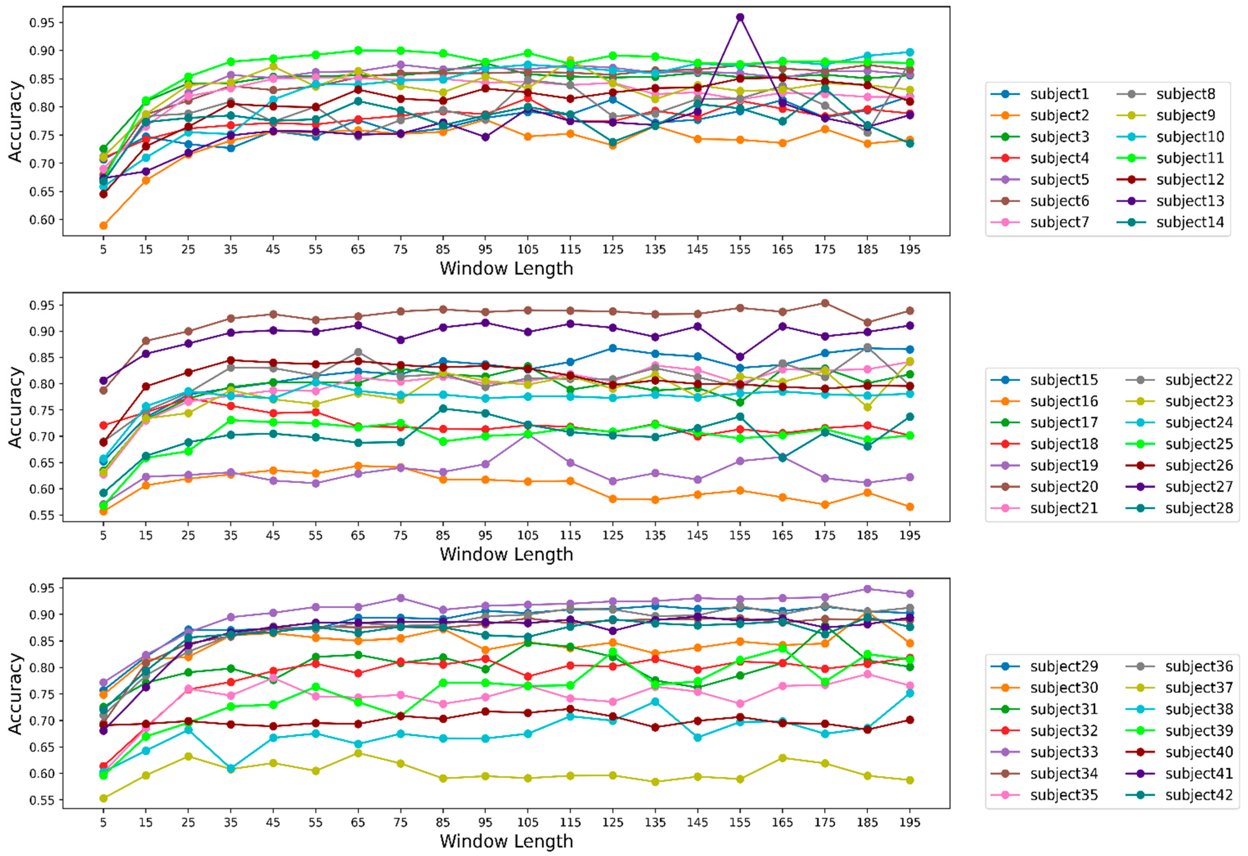
Figure 8 that the recorded results showed that window length had a significant impact on the performance of the models in HAR. However, the impact was noticeable until we reached a window length between 55 to 85 in the study. After that, the performance was not influenced substantially by incremental increases in window length. We can call the window length range of 55 to 85 the saturation range for the models’ performance. The reason behind such a trend could be that, after a certain length, even if we increase the window length, the model could not extract significant knowledge to enhance its performance. Although
Figure 8 displays the averaged effect of window length, we observe the influence on individual participants in
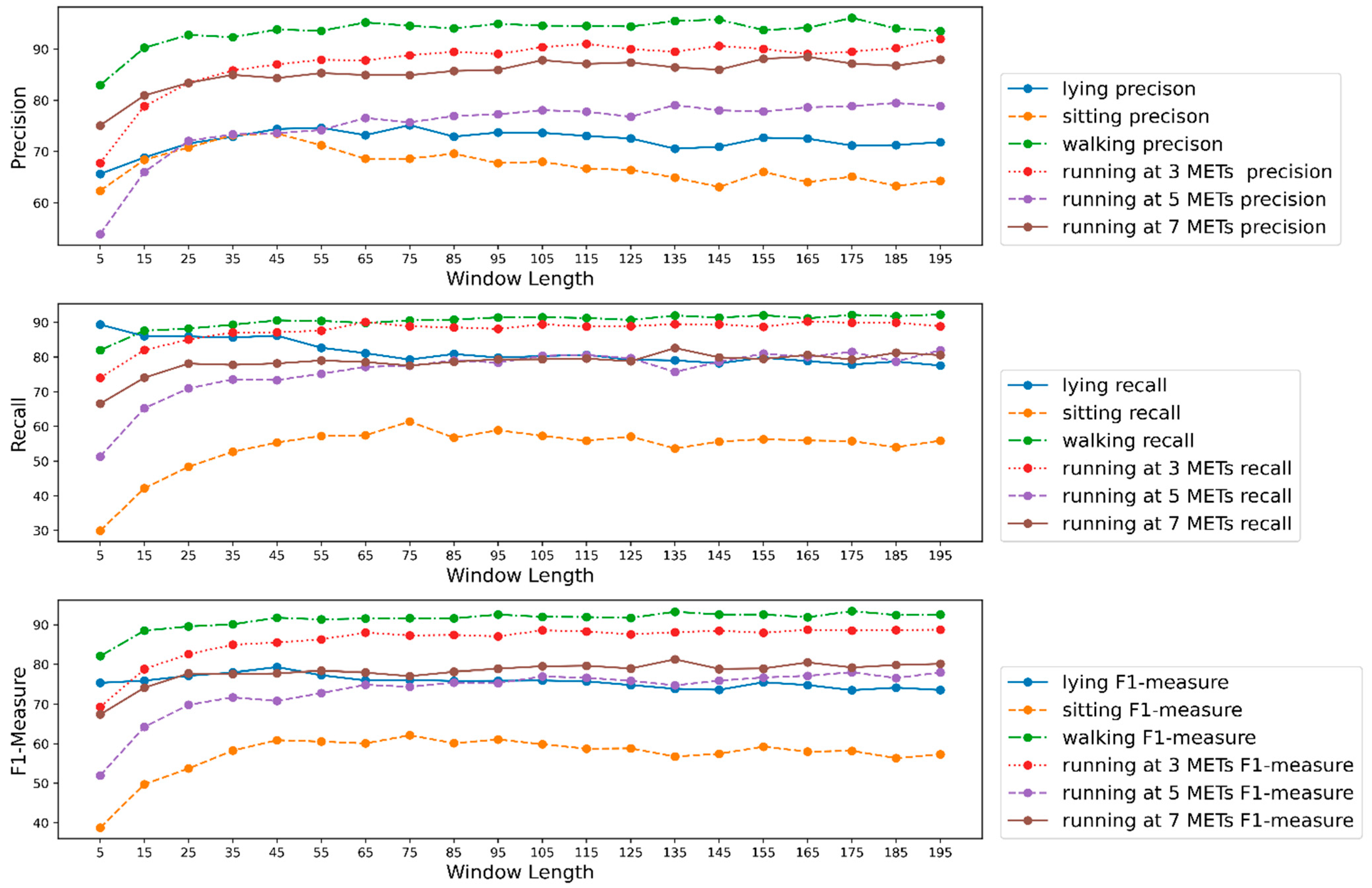
Figure 9. We experienced a similar trend for almost all participants. We had a contradictory trend in performance for participants 16 and 37. After the saturation range with the increment in window length models, performance for those participants was reduced. Although the decrement was not considered important, it was not usual if we observe the performance trend for other participants. This could happen due to noisy samples in the datasets belonging to those two participants, which need to be further analyzed. Observing the effect of window length on each activity class, we found that precision, recall, and f1-measure had very poor values for the sitting activity. In addition, the values of evaluation metrics reduced with an increase in window length for lower-intensity activities like sitting and lying. For instance, recall for lying was about 90% when the window length was the smallest but as the window length increased, the recall decreased. The effect of window length on lower-intensity activities was an interesting observation which was not evaluated in previous studies. We can assume that window length had different effects for activities with different intensities considering our outcome. When choosing a window length, we should also consider a window length that will help generate a better outcome for lower- and higher-intensity activities. Another reason behind such poor performance could be the lower number of samples for the activity sitting which we can see in
Table 3. Balancing the classes could have helped to improve the situation. Still, we did not do it in our study as our main objective was to observe the influence of window length rather than increasing the models’ performance.
From
Table 6, we can see that for most of the activity classes, the highest metric values we found were when the window length was above 150, but the highest values were not considerably greater than the values we found at saturation point. That means we need not choose a very high window length to achieve the best performance from the model; rather, we need to select a window length around the saturation range that will be considerably smaller than the window lengths where we found the highest metric values. If we manage to keep the window length smaller, it would reduce the time complexity for the models and increase the computational efficiency.
Although we have conducted analysis participant-wise and activity-wise, some analysis is yet to be done. For instance, we achieved very high performance for some participants, such as participants 26, 27, and 33 and very poor performance for participants 16, 19, and 37. Still, we did not try to determine why the model performed differently, especially for these participants; as we mentioned earlier, our objective was to study the effect of window length in 1D-CNN-LSTM in HAR.
In brief, we found that window length in 1D-CNN-LSTM had a significant effect on HAR. We found that the training time was affected by the window length. As the window length increased, the training time also increased. The approximate training time for the model using the lowest window length of 5 was about 40 minutes and almost 20 hours for the highest window length of 195. For our suggested saturation range of 55 to 85, the training time was about 4 hours. Here, we approximated the mentioned training time for each iteration of inter-subject validation, which means there were data from 41 subjects in training data, and test data included data from one subject, which we did not include in the training data. So, window length should not be arbitrarily long; rather, it should be chosen wisely by correctly identifying the saturation range so that the model offers less time complexity while training and more efficiency. In addition, for the 1D-CNN-LSTM model, other studies may choose a window length from our suggested saturation range of 55 to 85 for HAR. We resampled the whole dataset to 30 Hz, so our proposed saturation range should be 1.83 s to 2.83 s.
There are a number of limitations to our current study. We only used one accelerometer for our study to keep the computation complexity low as we conducted inter-participant validation for 42 participants. However, we may experience improvements in our study if a gyroscope sensor was also used with the accelerometer sensor since a gyroscope sensor can provide substantial information regarding the rotational nature. Moreover, the data were collected from only one position, a phone in the pocket, and we did not study how much the analysis would be affected if we used data from different body parts. In addition, we studied the effect of window length on one type of model, but other models also take windows of data as an input. We do not know if the effect would be the same for those models. However, we initiated this type of analysis using many participants, one accelerometer sensor, data from one position, and only one type of model. In future, we will try to conduct the same study using different models and settings.


