
Estimation of Sound Transmission Loss in Nanofiber Nonwoven Fabrics: Comparison of Conventional Models and the Simplified Limp Frame Model

Abstract
:1. Introduction
2. Samples and Measurement Setup
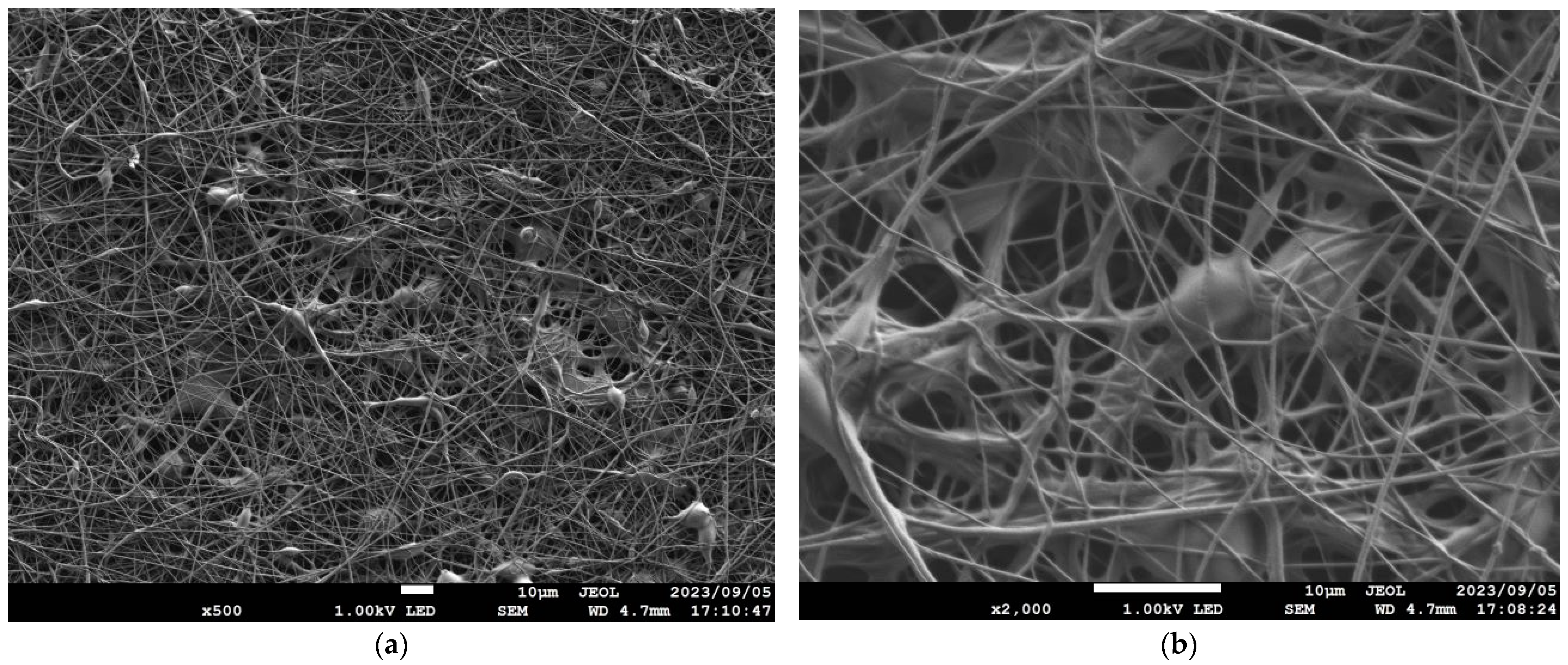
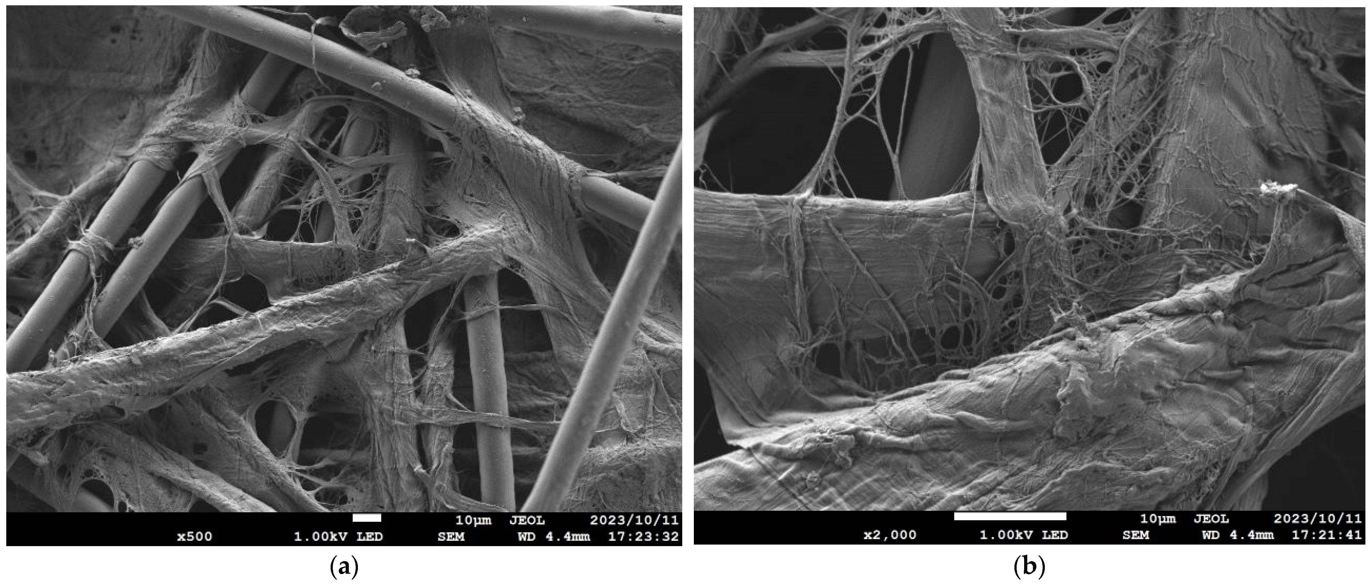
2.1. Samples
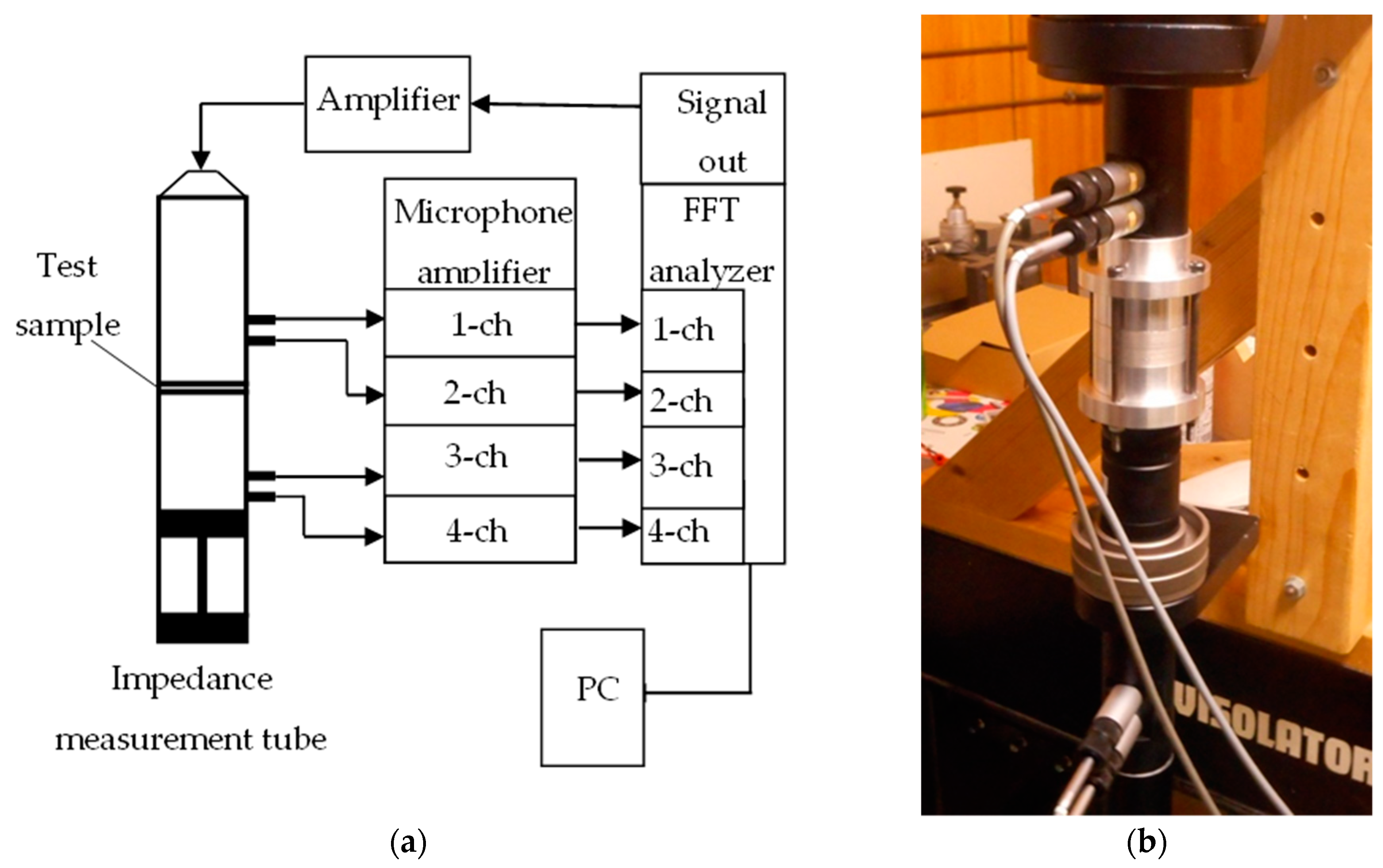
2.2. Equipment for Measuring Transmission Loss
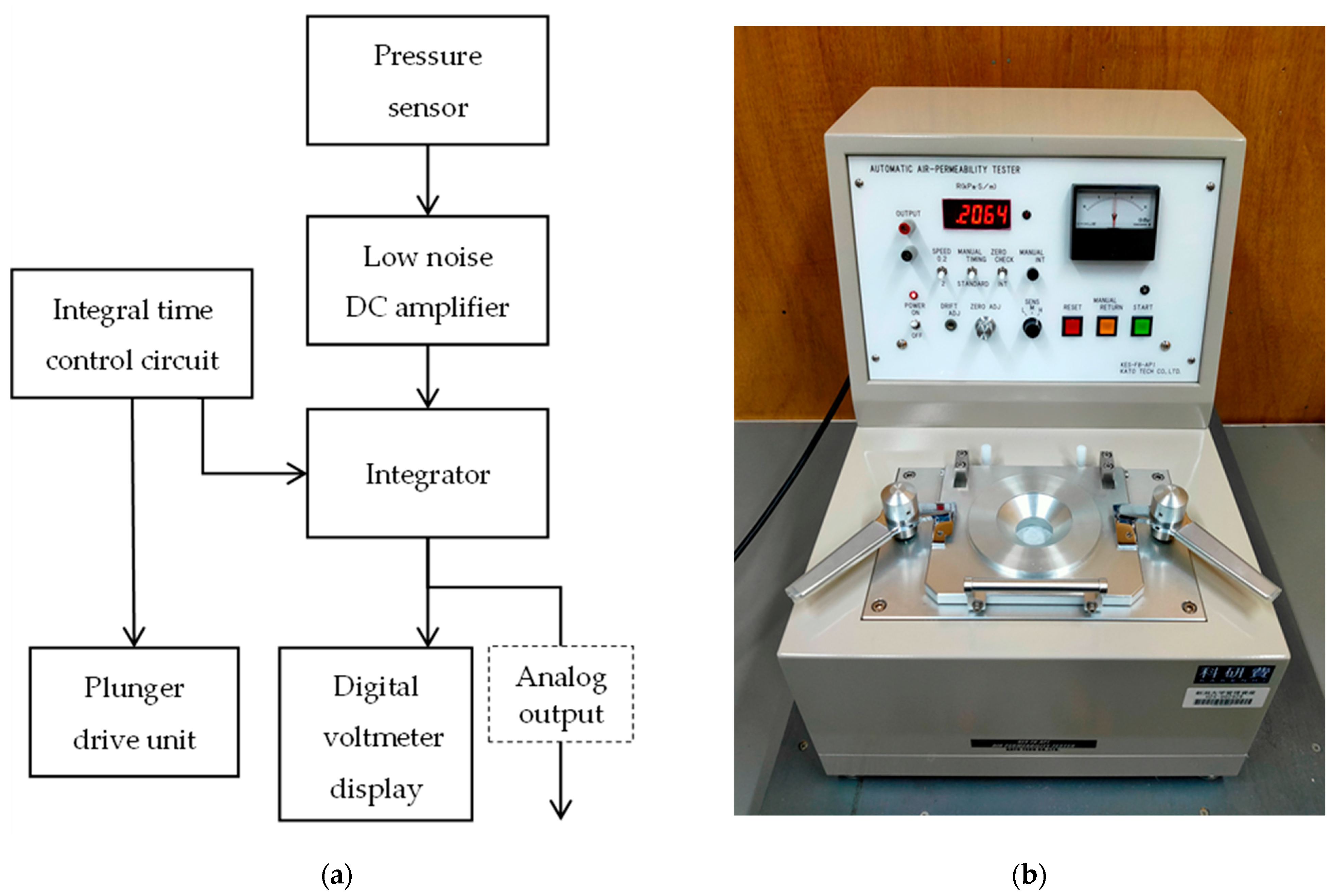
2.3. Equipment for Measuring Ventilation Resistance
3. Theoretical Analysis
3.1. Conventional Estimation Model for Nonwoven Fabrics
3.2. Limp Frame Model and Its Simplification
3.3. Simplified Limp Frame Model
3.4. Propagation Constant and Characteristic Impedance
3.5. Calculation of Transmission Loss
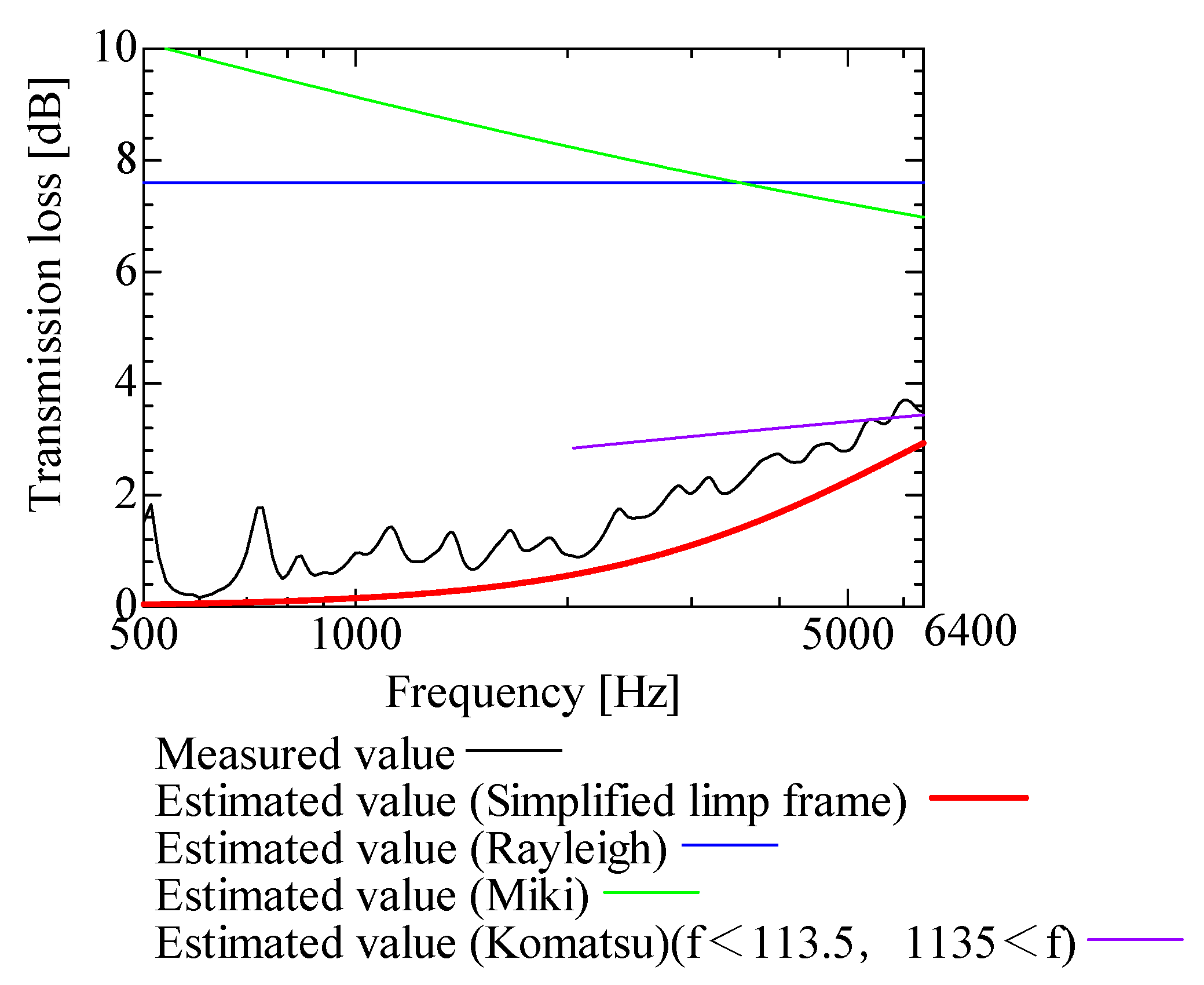
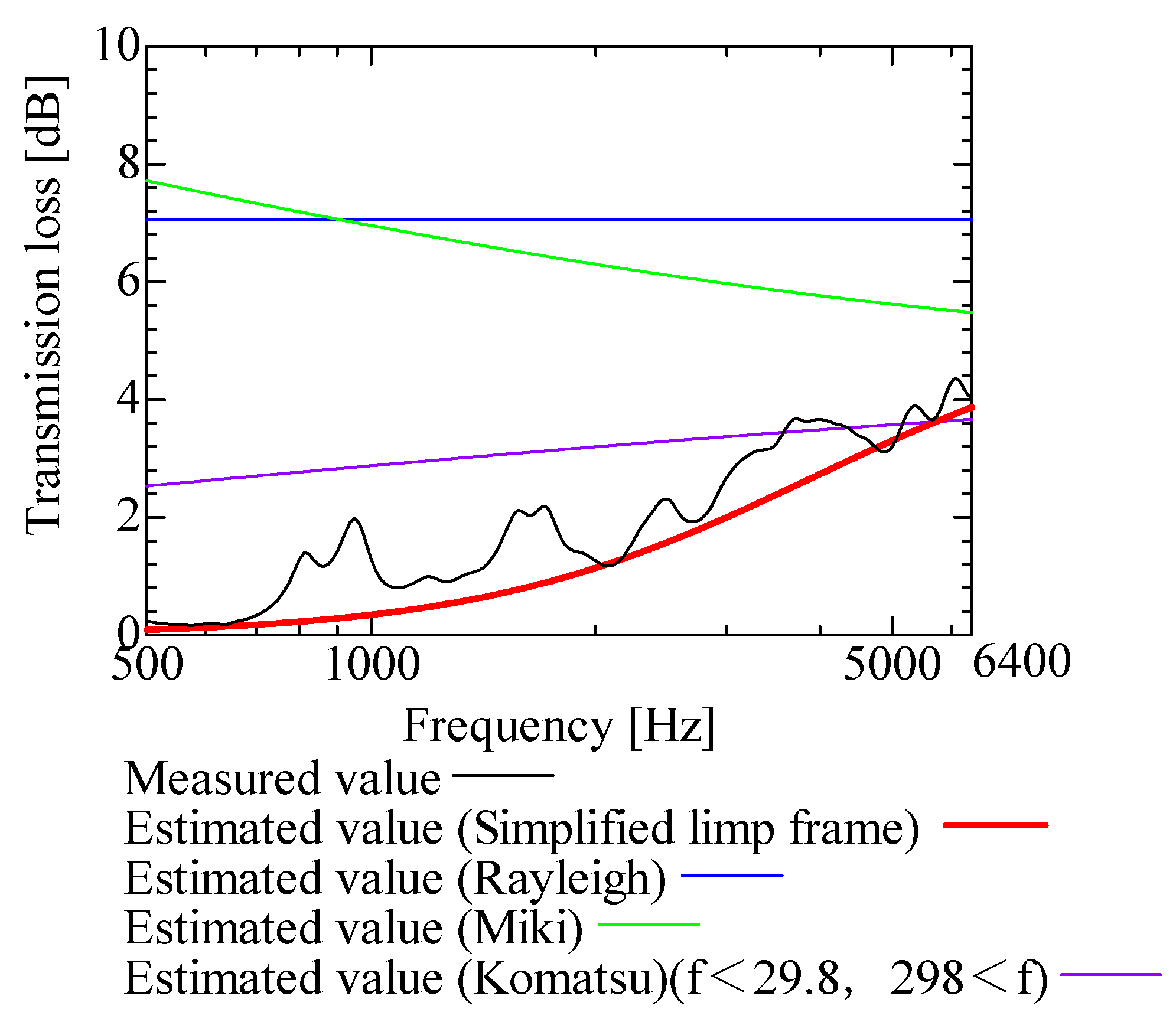
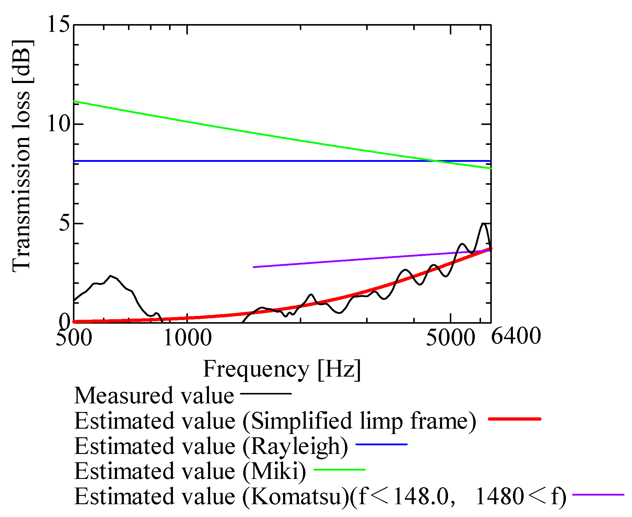
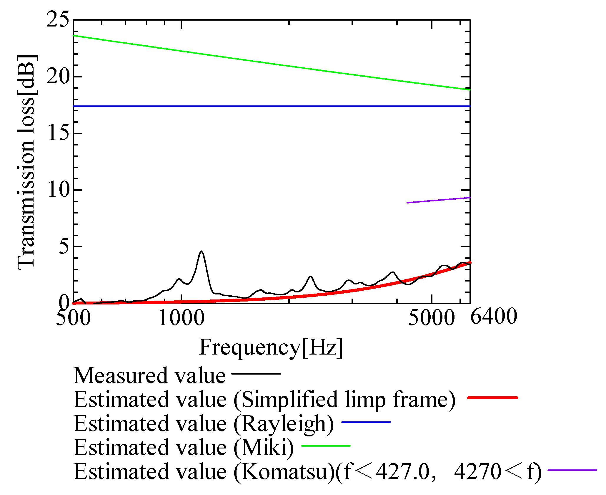
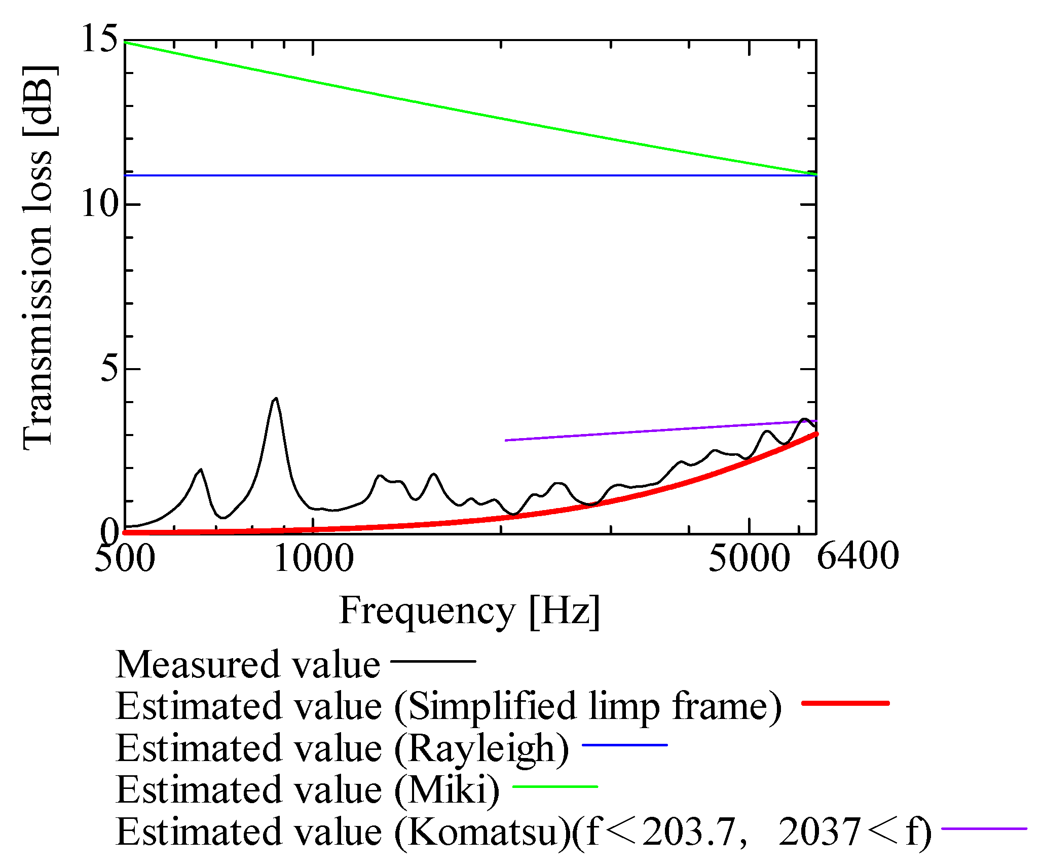
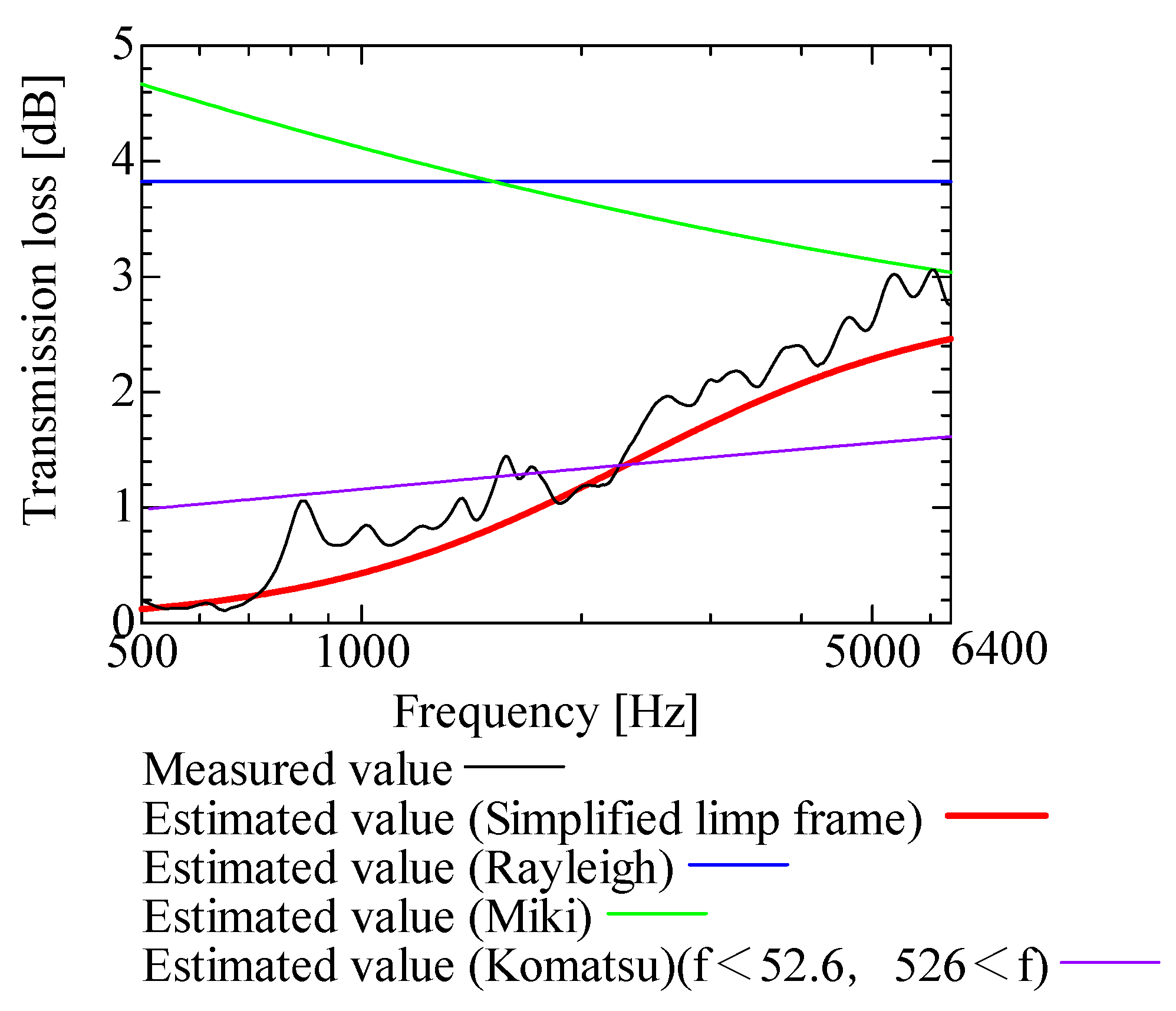
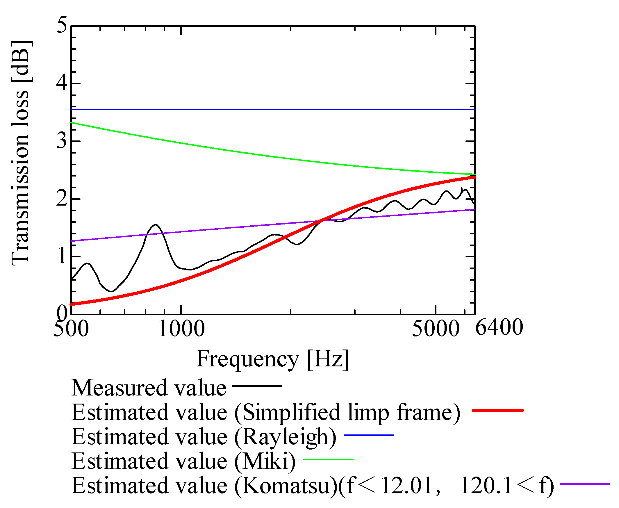
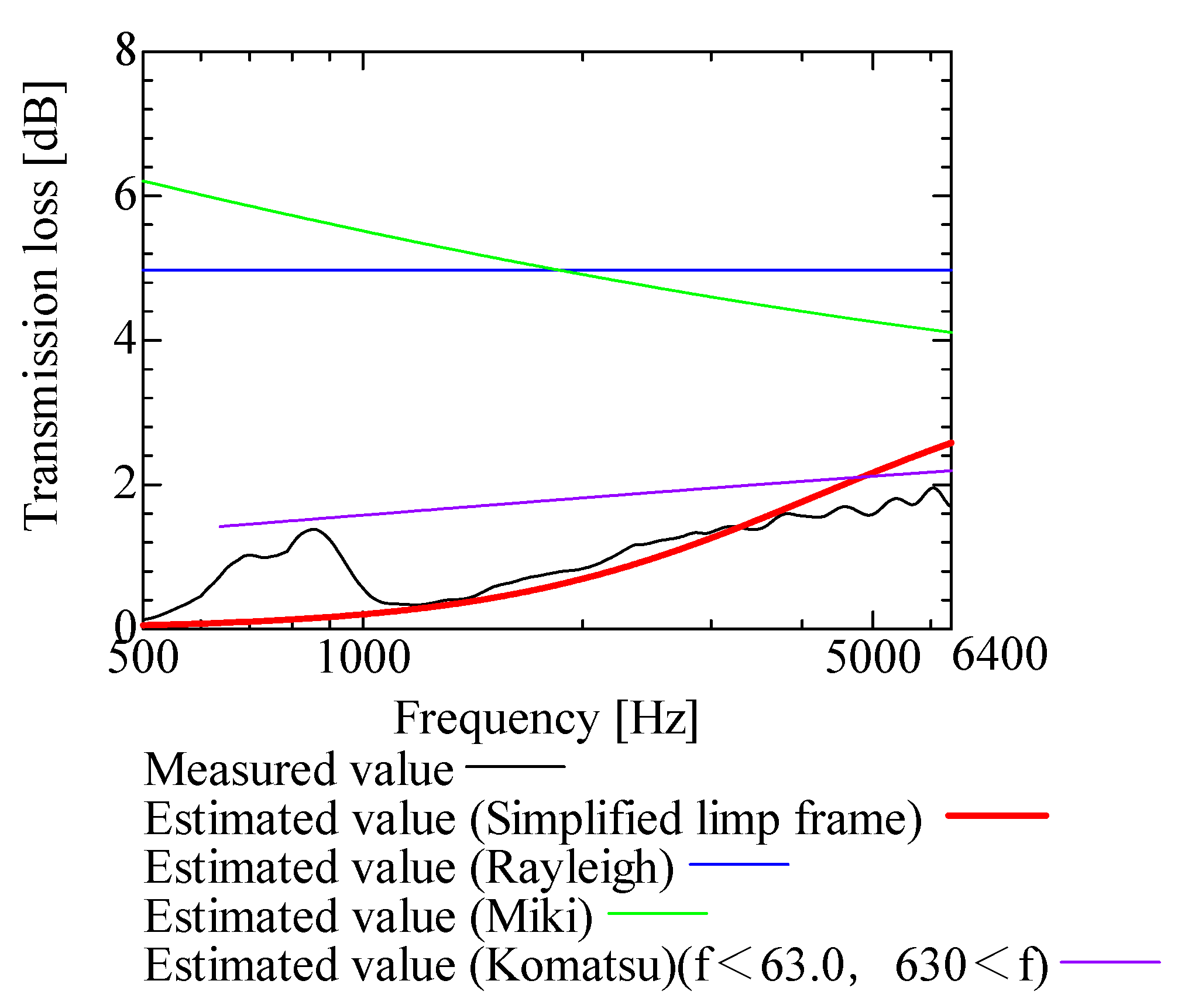
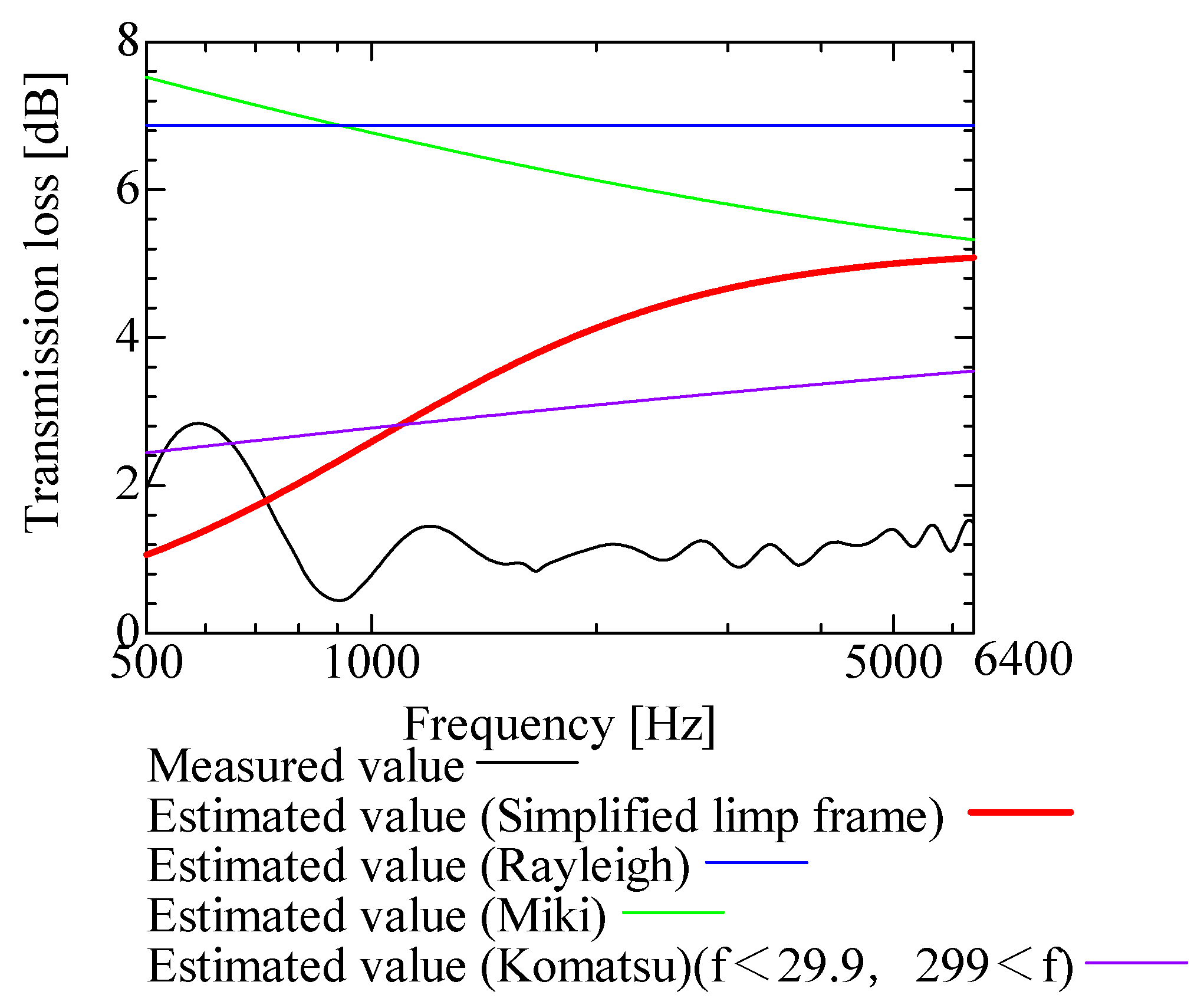
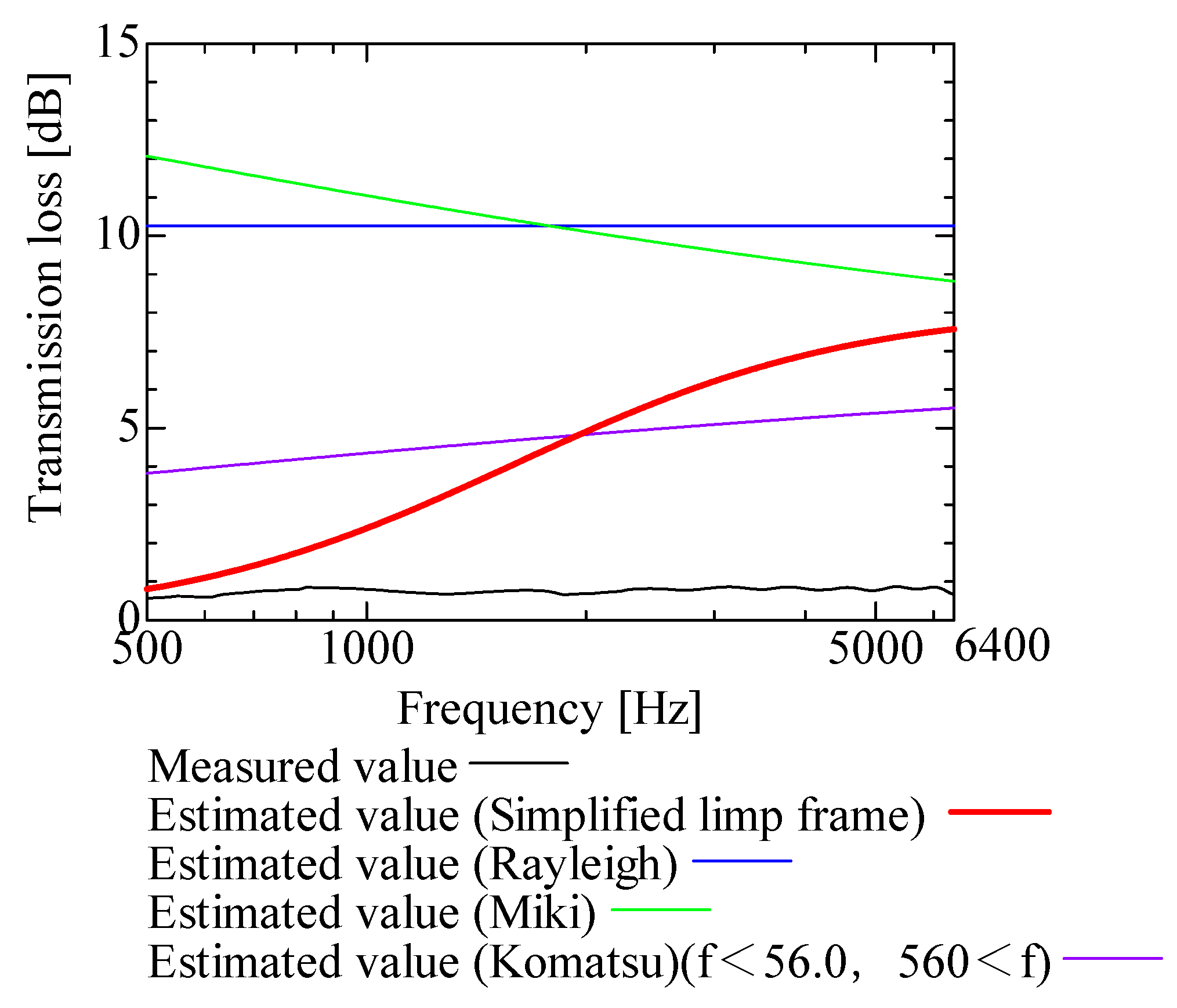
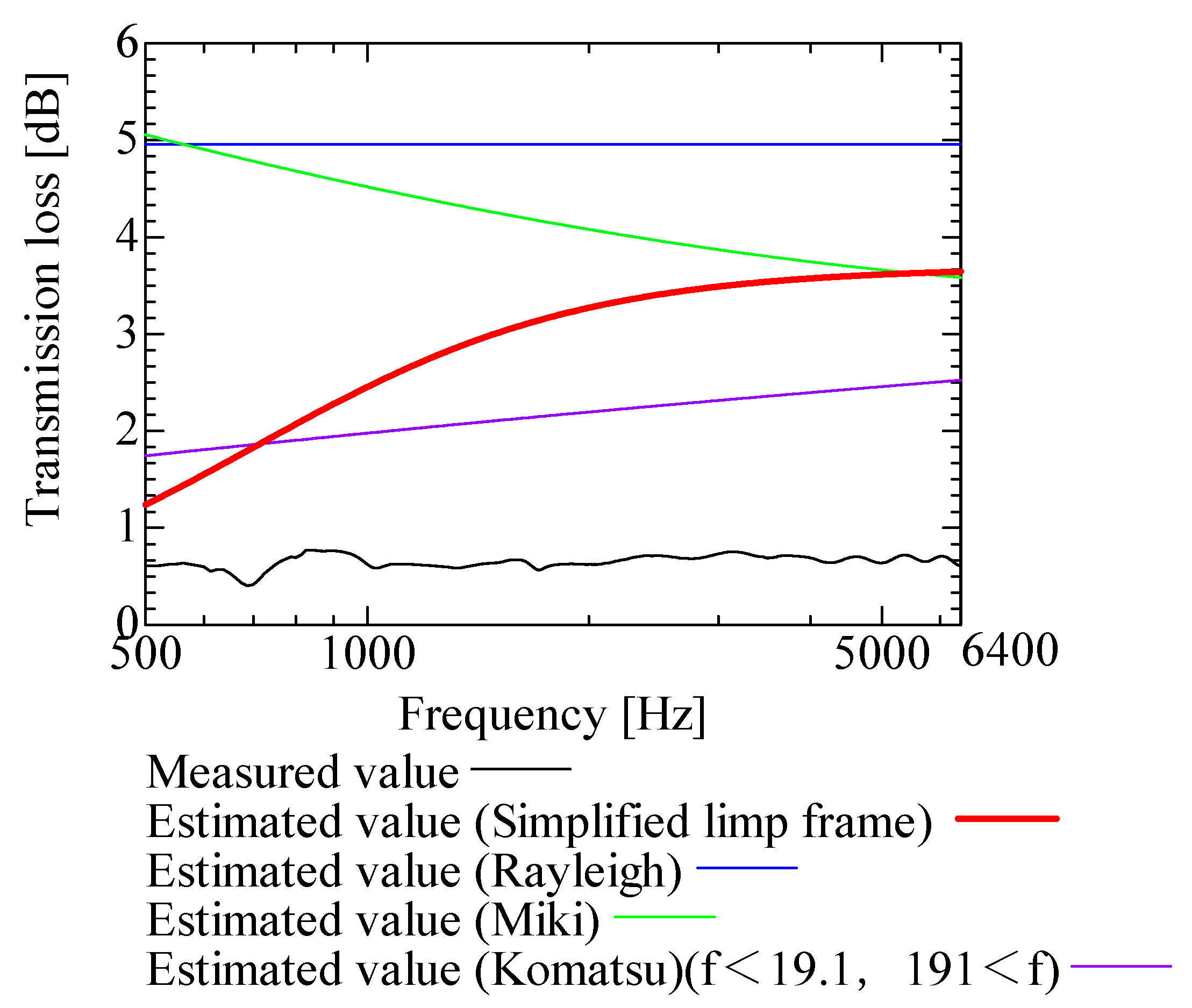
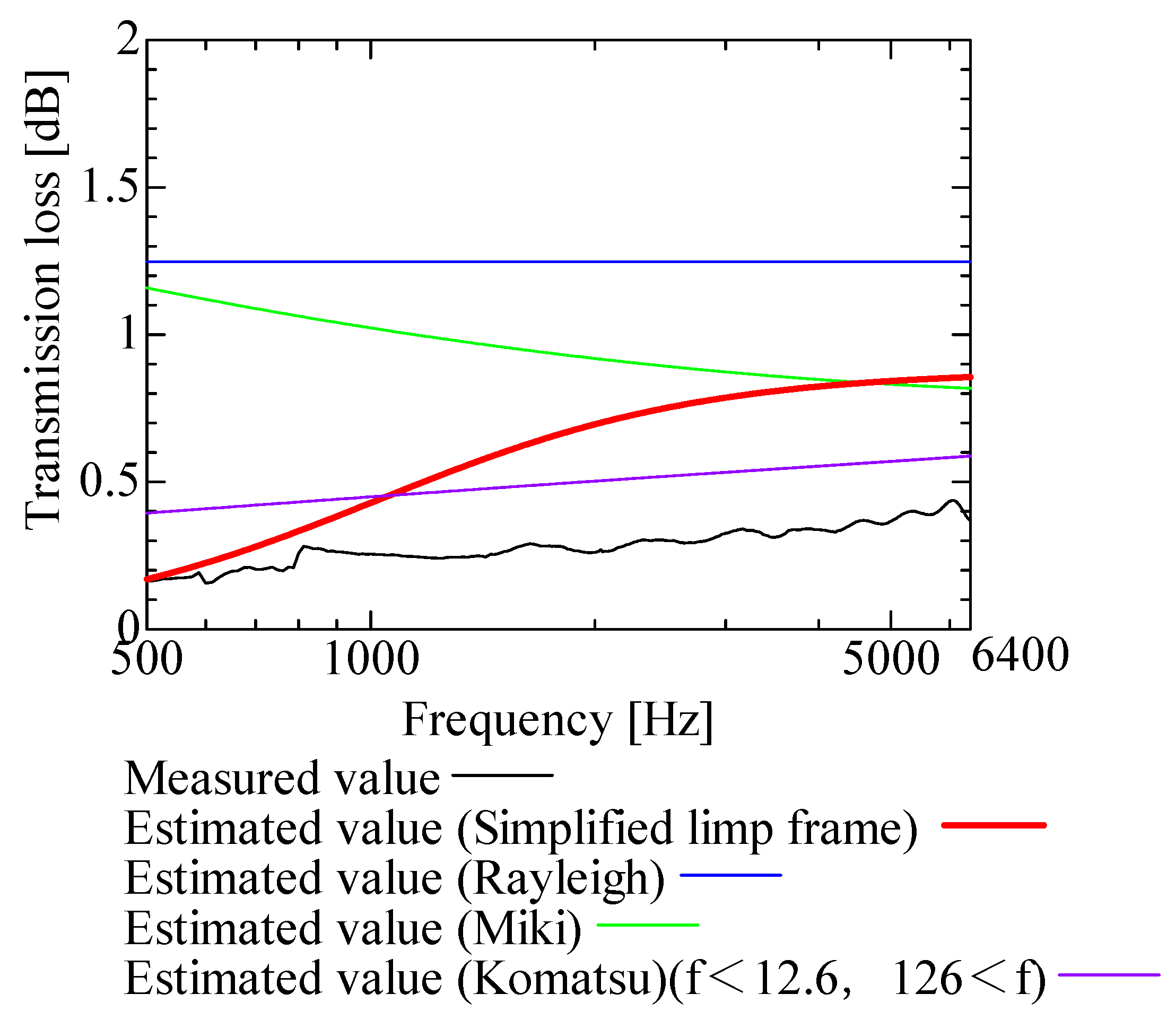
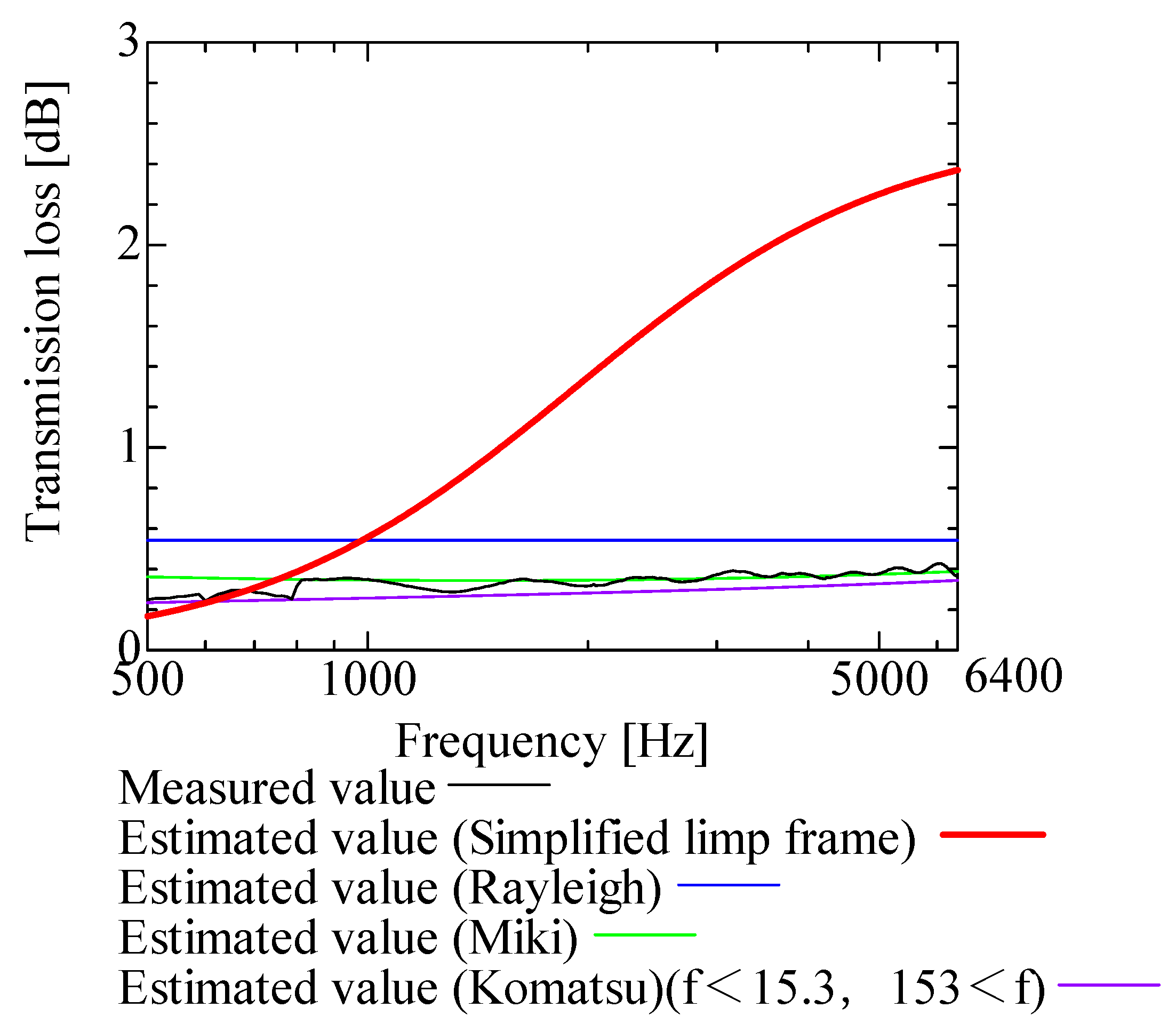
4. Comparison of Measured and Estimated Values
5. Conclusions
- (1)
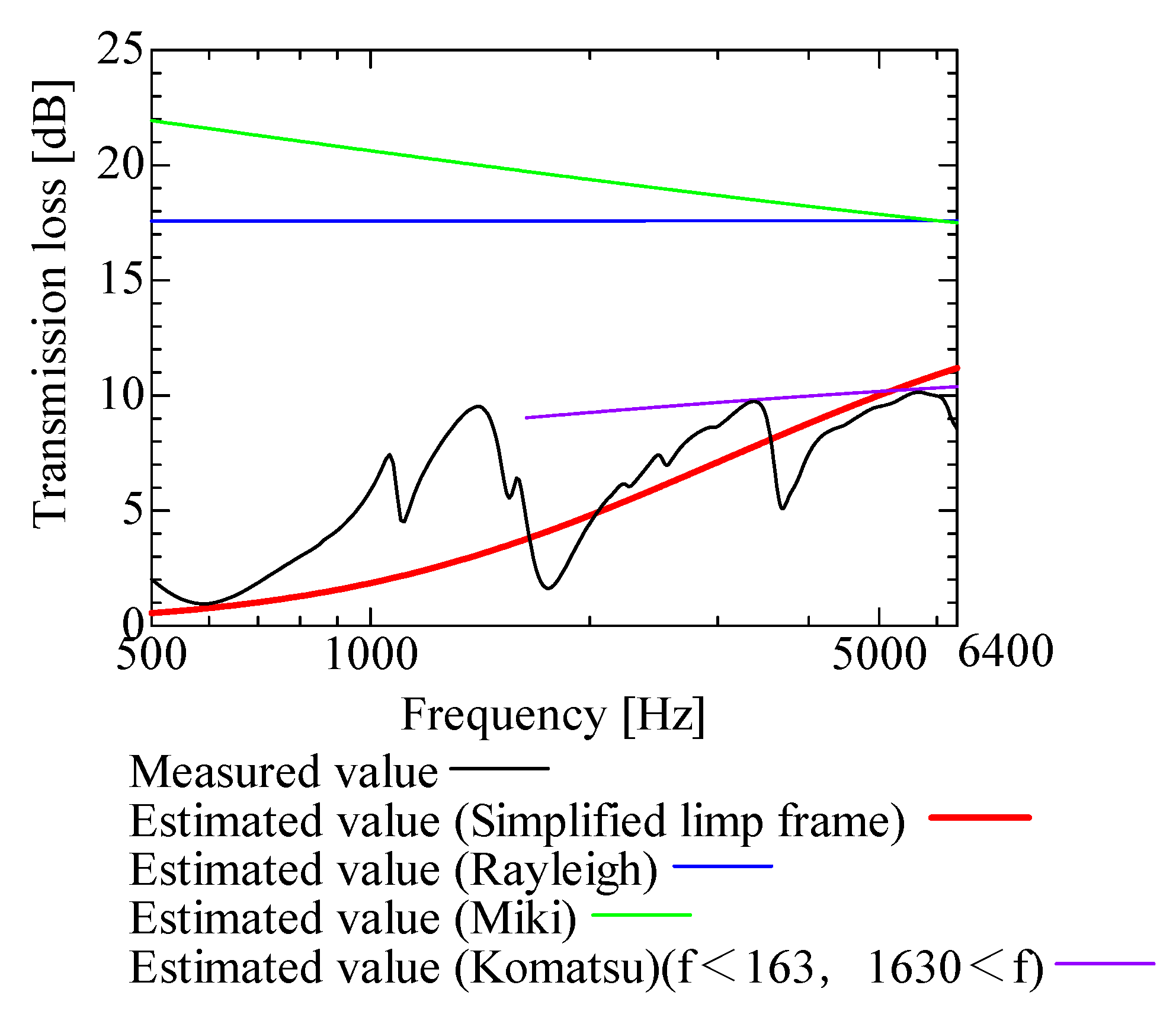
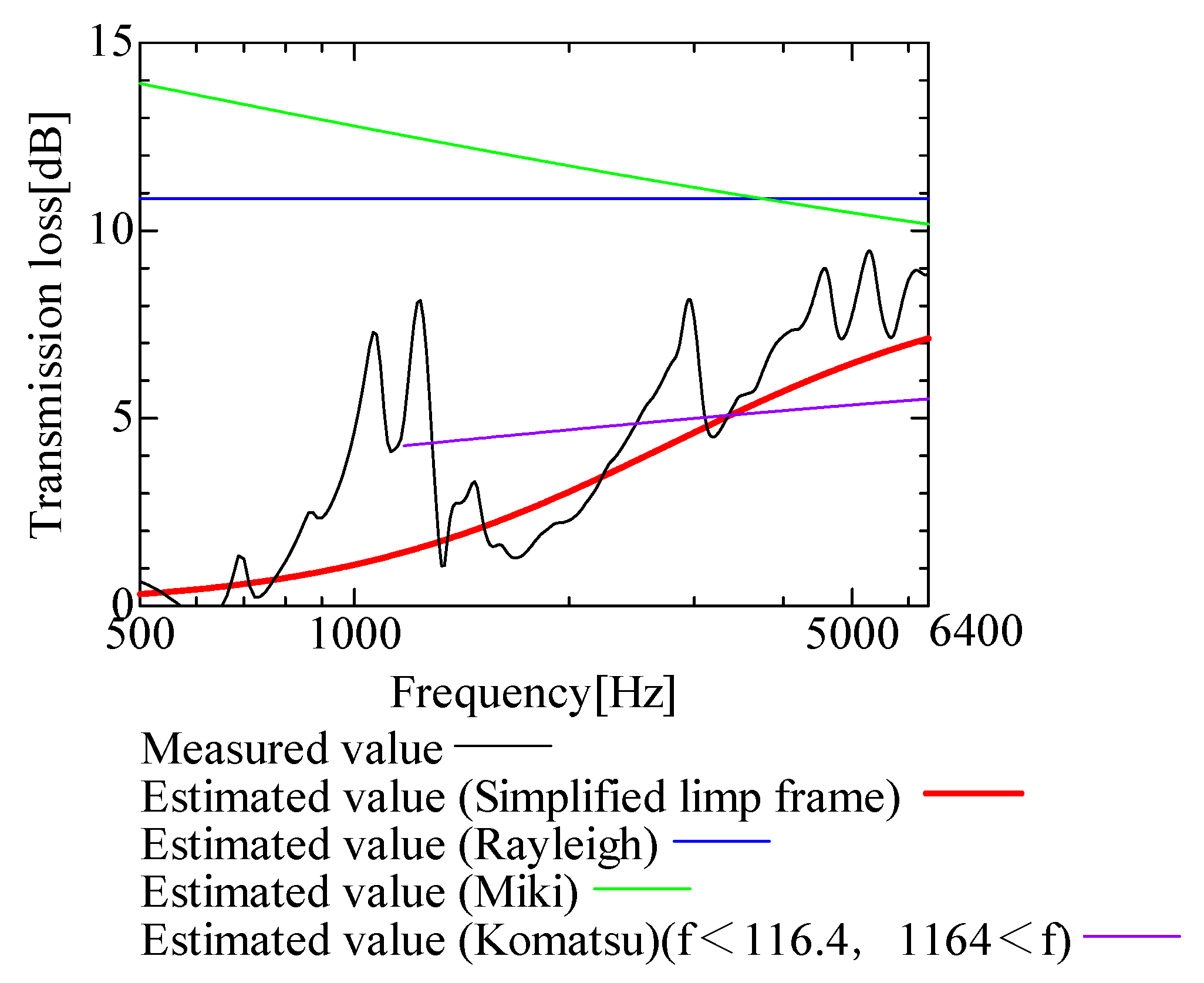
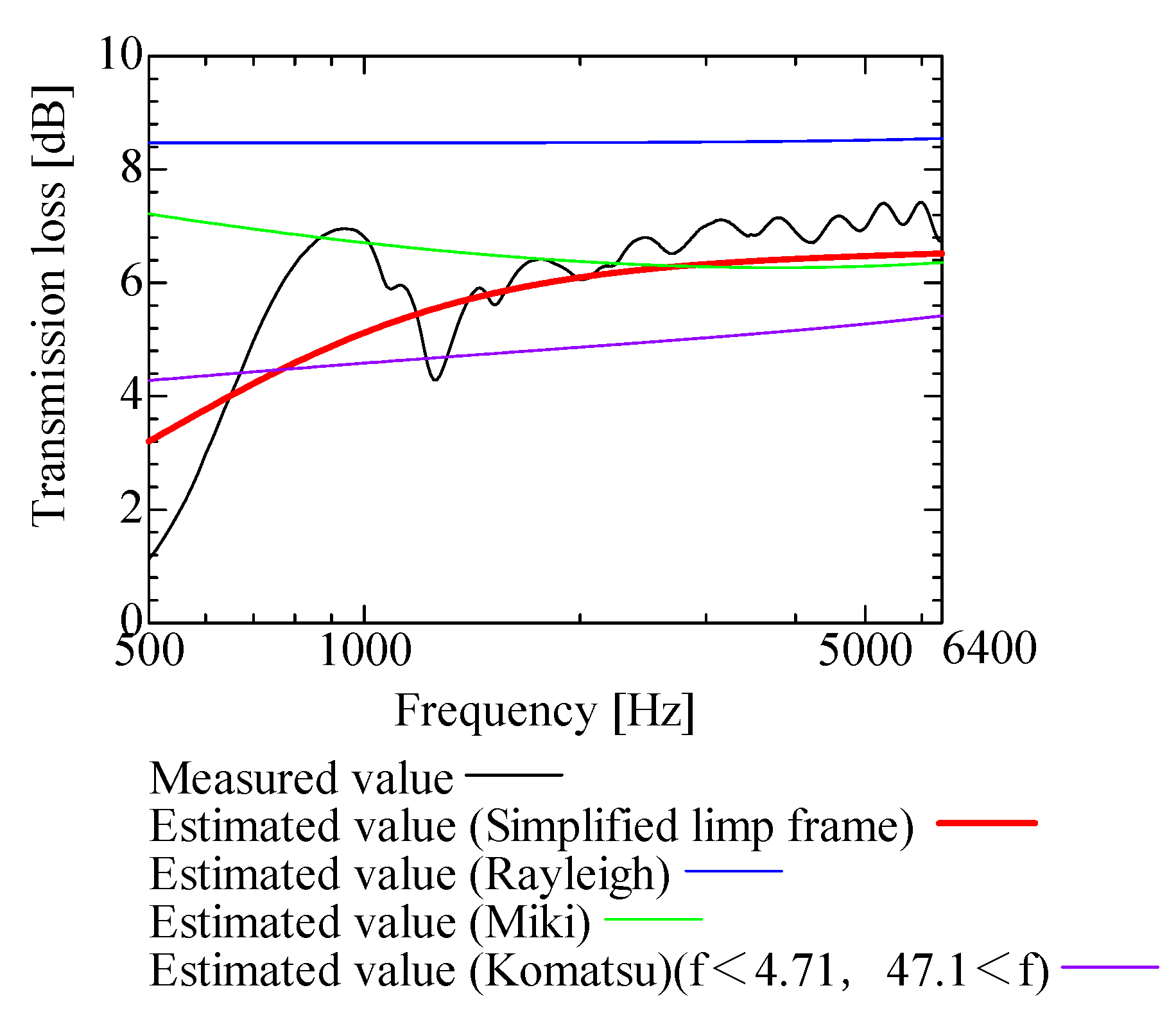
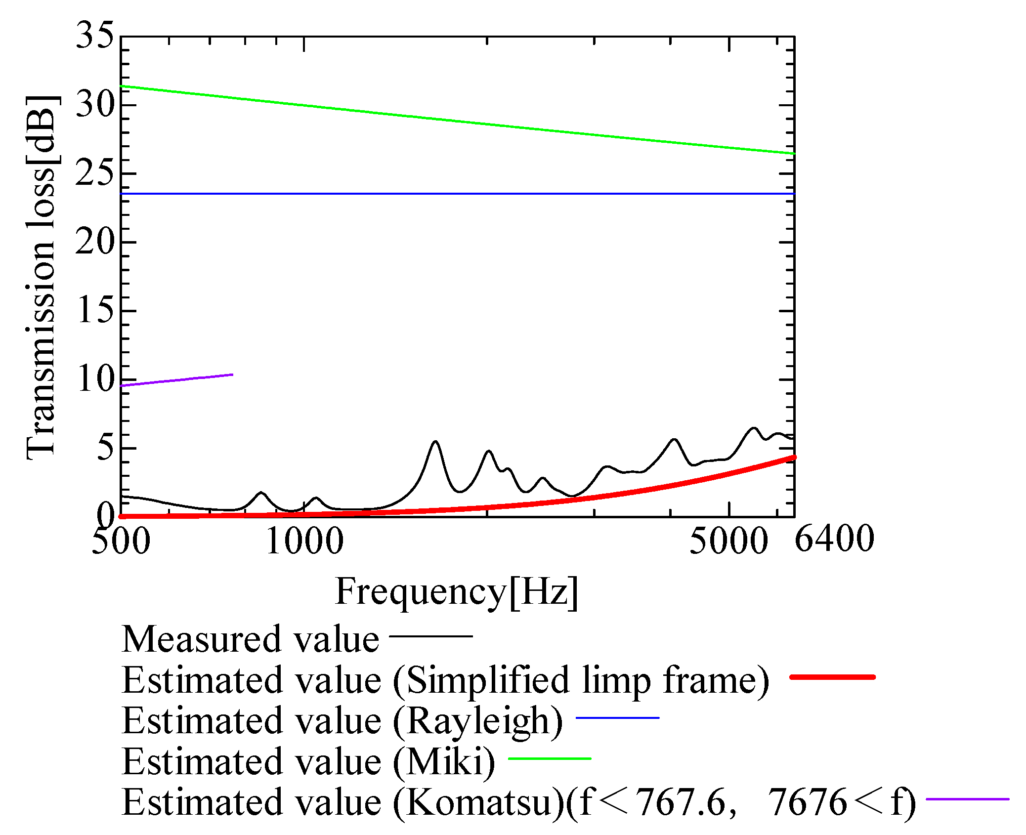
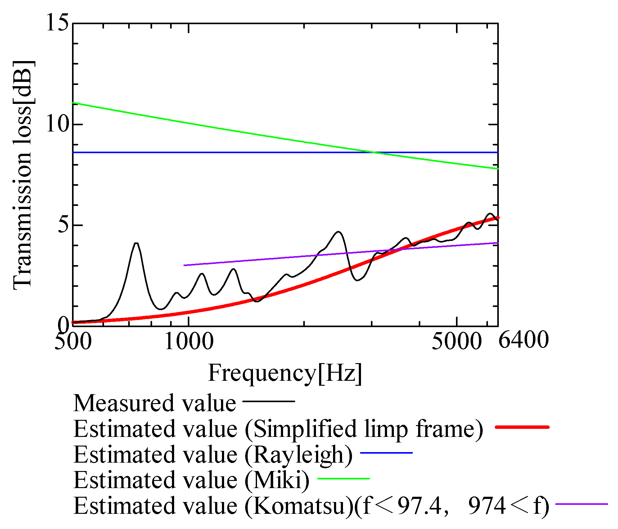
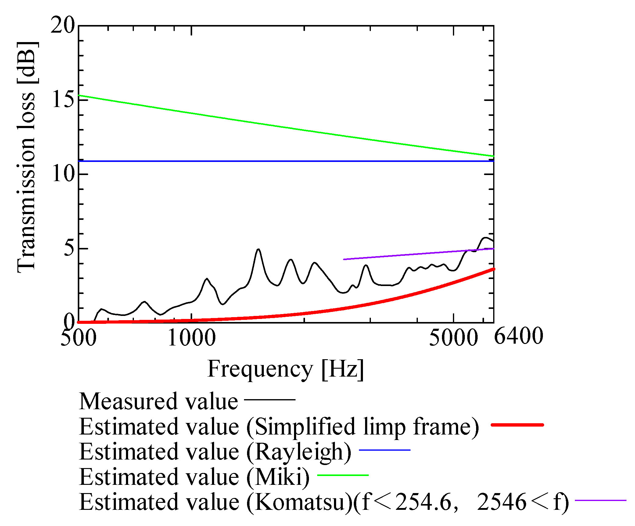
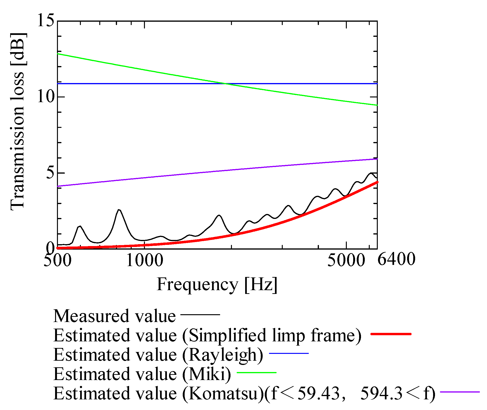
- The proposed SLFM is more suitable for estimating the transmission loss of NF-NWFs than the conventional Rayleigh, Miki, and Komatsu models. This study highlights the usefulness of the SLFM in estimating the acoustic insulation performance of NF-NWFs. The SLFM serves as an efficient method for predicting transmission loss to determine the more suitable application between masks and filters, which possess conflicting requirements for transmission loss;
- (2)
- The SLFM can estimate the transmission loss of both MFC-NWFs and other NF-NWFs;
- (3)
- Experiments have revealed the acoustic insulation capabilities of MFC-NWFs constructed from cellulose. This research could be valuable for potentially substituting synthetic fiber filters and masks with those made from cellulose in the future.
Author Contributions
Funding
Data Availability Statement
Acknowledgments
Conflicts of Interest
References
- Cao, L.; Fua, Q.; Si, Y.; Ding, B.; Yu, J. Porous materials for sound absorption. Compos. Commun. 2018, 10, 25–35. [Google Scholar] [CrossRef]
- Parikh, D.V.; Chen, Y.; Sun, L. Reducing Automotive Interior Noise with Natural Fiber Nonwoven Floor Covering Systems. Text. Res. J. 2006, 76, 813–820. [Google Scholar] [CrossRef]
- Lee, J.W.; Park, S.W. Effect of Fiber Cross Section Shape on the Sound Absorption and the Sound Insulation. Fibers Polym. 2021, 22, 2937–2945. [Google Scholar] [CrossRef]
- Iannace, G. Acoustic properties of nanofibers. Noise Vib. Worldw. 2014, 45, 29–33. [Google Scholar] [CrossRef]
- Ji, G.; Cui, J.; Fang, Y.; Yao, S.; Zhou, J.; Kim, J. Nano-fibrous composite sound absorbers inspired by owl feather surfaces. Appl. Acoust. 2019, 156, 151–157. [Google Scholar] [CrossRef]
- Hajimohammad, M.; Soltani, P.; Semnani, D.; Taban, E.; Fashandi, H. Nonwoven fabric coated with core-shell and hollow nanofiber membranes for efficient sound absorption in buildings. Build. Environ. 2022, 213, 12. [Google Scholar] [CrossRef]
- Özkal, A.; Çallıoglu, F.C. Effect of nanofiber spinning duration on the sound absorption capacity of nonwovens produced from recycled polyethylene terephthalate fibers. Appl. Acoust. 2020, 169, 107468. [Google Scholar] [CrossRef]
- Liu, H.; Zuo, B. Sound absorption property of PVA/PEO/GO nanofiber membrane and non-woven composite material. J. Ind. Text. 2020, 50, 512–525. [Google Scholar] [CrossRef]
- Shao, X.; Yan, X. Sound absorption properties of nanofiber membrane-based multi-layer composites. Appl. Acoust. 2022, 200, 109029. [Google Scholar] [CrossRef]
- Passaro, J.; Russo, P.; Bifulco, A.; De Martino, M.T.; Granata, V.; Vitolo, B.; Iannace, G.; Vecchione, A.; Marulo, F.; Branda, F. Water Resistant Self-Extinguishing Low Frequency Soundproofing Polyvinylpyrrolidone Based Electrospun Blankets. Polymers 2019, 11, 1205. [Google Scholar] [CrossRef]
- Corey, R.M.; Jones, U.; Singer, A.C. Acoustic effects of medical, cloth, and transparent face masks on speech signals. J. Acoust. Soc. Am. 2020, 148, 2371–2375. [Google Scholar] [CrossRef]
- Atcherson, S.R.; McDowell, B.R.; Howard, M.P. Acoustic effects of non-transparent and transparent face coverings. J. Acoust. Soc. Am. 2021, 149, 2249–2254. [Google Scholar] [CrossRef]
- Ullah, S.; Ullah, A.; Lee, J.; Jeong, Y.; Hashmi, M.; Zhu, C.; Joo, K.I.; Cha, H.J.; Kim, I.S. Reusability Comparison of Melt-Blown vs Nanofiber Face Mask Filters for Use in the Coronavirus Pandemic. ACS Publ. 2020, 3, 7231–7241. [Google Scholar] [CrossRef] [PubMed]
- Rayleigh, J.W.S. The Theory of Sound, 2nd ed.; Dover: New York, NY, USA, 1945; Volume II. [Google Scholar]
- Miki, Y. Acoustical properties of porous materials-Modifications of Delany-Bazley models. J. Acoust. Soc. Jpn. 1990, 11, 19–24. [Google Scholar] [CrossRef]
- Komatsu, T. Improvement of the Delany-Bazley and Miki models for fibrous sound-absorbing materials. Acoust. Sci. Tech. 2008, 29, 121–129. [Google Scholar] [CrossRef]
- Panneton, R. Comments on the limp frame equivalent fluid model for porous media. J. Acoust. Soc. Am. 2007, 122, EL217. [Google Scholar] [CrossRef]
- Kurosawa, Y. Development of sound absorption coefficient prediction technique of ultrafine fiber. Trans. JSME 2016, 82, 7. (In Japanese) [Google Scholar]
- Sakamoto, S.; Shintani, T.; Hasegawa, T. Simplified Limp Frame Model for Application to Nanofiber Nonwovens (Selection of Dominant Biot Parameters). Nanomaterials 2022, 12, 3050. [Google Scholar] [CrossRef]
- Biot, M.A. Theory of propagation of elastic waves in a fluid-saturated porous solid. I. Low-frequency range. J. Acoust. Soc. Am. 1956, 28, 168–178. [Google Scholar] [CrossRef]
- Biot, M.A. Theory of propagation of elastic waves in a fluid-saturated porous solid. II. Higher frequency range. J. Acoust. Soc. Am. 1956, 28, 179–191. [Google Scholar] [CrossRef]
- Yeon, J.O.; Kim, K.W.; Yang, K.S.; Kim, J.M.; Kim, M.J. Physical properties of cellulose sound absorbers produced using recycled paper. Constr. Build. Mater. 2014, 70, 494–500. [Google Scholar] [CrossRef]
- Zong, D.; Bai, W.; Yin, X.; Yu, J.; Zhang, S.; Ding, B. Gradient Pore Structured Elastic Ceramic Nanofiber Aerogels with Cellulose Nanonets for Noise Absorption. Adv. Funct. Mater. 2023, 33, 2301870. [Google Scholar] [CrossRef]
- Fan, B.; Yao, Q.; Wang, C.; Jin, C.; Wang, H.; Xiong, Y.; Li, S.; Sun, Q. Natural Cellulose Nanofiber Extracted from Cell Wall of Bamboo Leaf and Its Derived Multifunctional Aerogel. Polym. Compos. 2017, 39, 3869–3876. [Google Scholar] [CrossRef]
- Lefebvre, J.; Leblanc, A.; Genestie, B.; Chartier, T.; Lavie, A. Acoustic Properties of aerogel encapsulated by macroporous cellulose. In Proceedings of the 23rd International Congress on Sound and Vibration, ICSV23, Athens Greece, 10–14 July 2016. [Google Scholar]
- Zhang, C.; Yuan, X.; Wu, L.; Han, Y.; Sheng, J. Study on morphology of electrospun poly(vinyl alcohol) mats. Eur. Polym. J. 2005, 41, 423–432. [Google Scholar] [CrossRef]
- Delany, M.E.; Bazley, E.N. Acoustical properties offibrous absorbent materials. Appl. Acoust. 1970, 3, 105–116. [Google Scholar] [CrossRef]
- Allard, J.F.; Atalla, N. Propagation of Sound in Porous Media; John Wiley & Sons, Ltd.: Hoboken, NJ, USA, 2009; ISBN 9780470747339. [Google Scholar]
- Sasao, H. Introduction to Acoustic Analysis by Excel-Analysis of Acoustic Structure Characteristics-(1) Fundamentals of Acoustic Analysis and Excel. Air-Cond. Sanit. Eng. 2006, 80, 75–85. (In Japanese) [Google Scholar]


| Properties of Test Samples (Nanofibers) | |||||
|---|---|---|---|---|---|
| Thickness [µm] | Area Density [g/m2] | Flow Resistivity [Ns/m4] | Material (Nano/Substrate) | Corresponding Figure Number | |
| Sample A | 60 | 18.2 | 5.26 × 10⁶ | PVDF/PET | 26 |
| Sample B | 60 | 18.6 | 1.48 × 10⁷ | PVDF/PET | 23 |
| Sample C | 230 | 80.06 | 1.91 × 10⁶ | PVDF/PET | 31 |
| Sample D | 230 | 80.12 | 2.99 × 10⁶ | PVDF/PET | 29 |
| Sample E | 230 | 80.3 | 5.60 × 10⁶ | PVDF/PET | 30 |
| Sample F | 230 | 81.1 | 1.63 × 10⁷ | PVDF/PET | 14 |
| Sample 1 | 56 | 18 | 2.55 × 10⁷ | PESU/PET | 19 |
| Sample 2 | 2000 | 100 | 4.71 × 10⁵ | PESU/PET | 16 |
| Shinwa 1-1 | 240 | 22 | 5.94 × 10⁶ | PVDF/PP | 20 |
| Shinwa 1-2 | 240 | 21.2 | 2.98 × 10⁶ | PVDF/PP | 22 |
| Shinwa 1-3 | 240 | 20.6 | 1.20 × 10⁶ | PVDF/PP | 27 |
| Shinwa 1-4 | 240 | 20.05 | 1.53 × 10⁶ | PVDF/PP | 33 |
| Shinwa 2-1 | 70 | 15.4 | 2.04 × 10⁷ | PVDF/PP:PE | 25 |
| Shinwa 2-2 | 70 | 14.2 | 1.14 × 10⁷ | PVDF/PP:PE | 21 |
| Shinwa 2-3 | 70 | 13.52 | 6.30 × 10⁶ | PVDF/PP:PE | 28 |
| Shinwa 2-4 | 70 | 13.05 | 1.26 × 10⁶ | PVDF/PP:PE | 32 |
| Tenma 1 | 99.4 | 34.1 | 9.74 × 10⁶ | cellulose/PP | 18 |
| Tenma 2 | 122.5 | 49.3 | 1.16 × 10⁷ | cellulose/PP | 15 |
| Tenma 3 | 104.3 | 25 | 7.68 × 10⁷ | cellulose/PP | 17 |
| Tenma 4 | 85.7 | 20 | 4.27 × 10⁷ | cellulose/PP | 24 |
| Properties of Test Samples (Base Materials) | |||||
| Thickness [µm] | Area Density [g/m2] | Flow Resistivity [Ns/m4] | Material (Nano/Substrate) | ||
| Sample G | 60 | 18 | 5.00 × 10⁵ | PVDF/PET | |
| Sample H | 230 | 80 | 1.87 × 10⁵ | PVDF/PET | |
| Shinwa 1-5 | 240 | 20 | 7.93 × 10⁴ | PVDF/PET | |
| Shinwa 2-5 | 70 | 13 | 2.99 × 10⁵ | PVDF/PET | |
| Base of Sample 1 | 56 | 15 | - | PVDF/PET | |
| Biot Parameters | Variables | Value | Unit | |
|---|---|---|---|---|
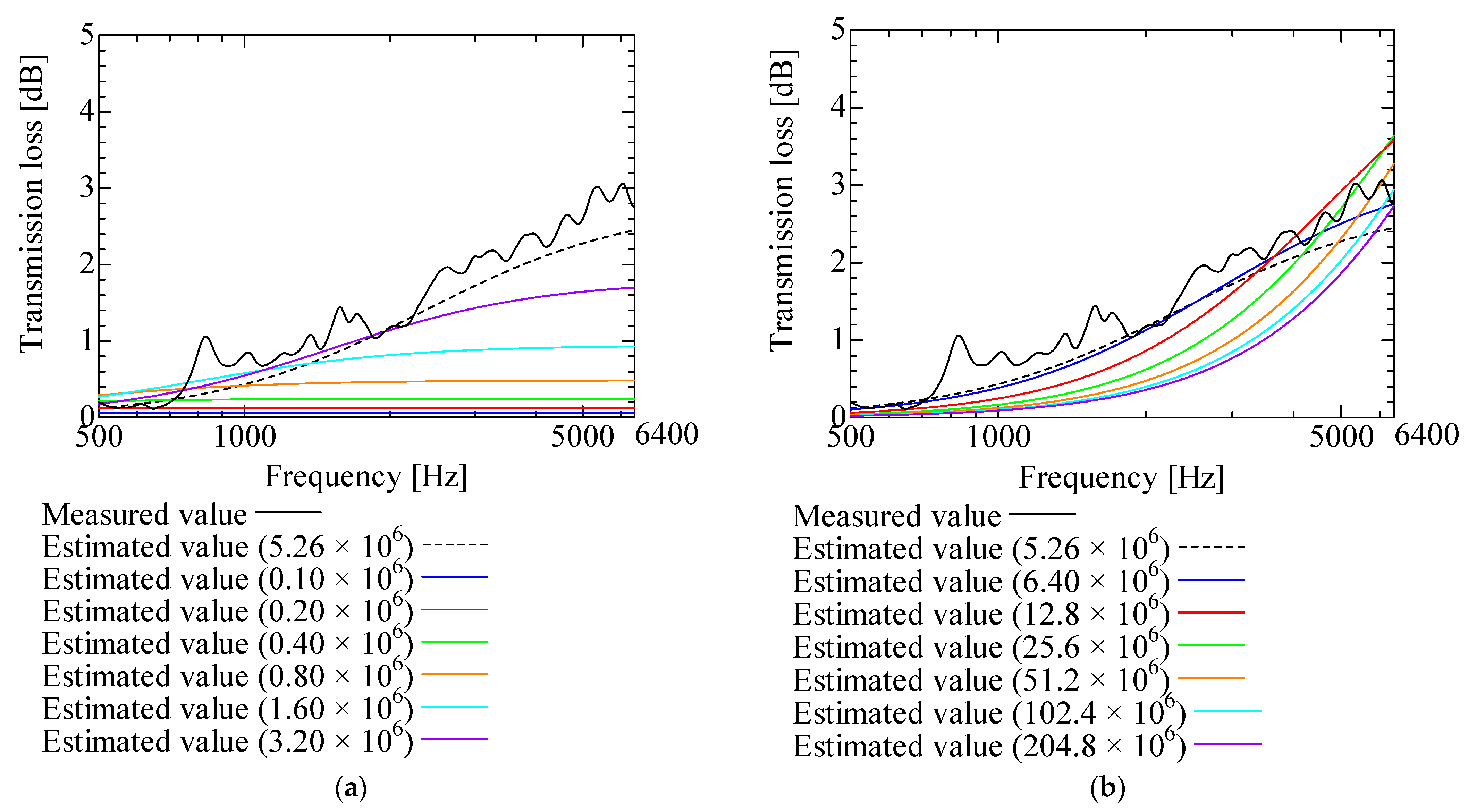
| Acoustical | Flow resistivity | 5.26 × 10⁶ | Ns/m4 | |
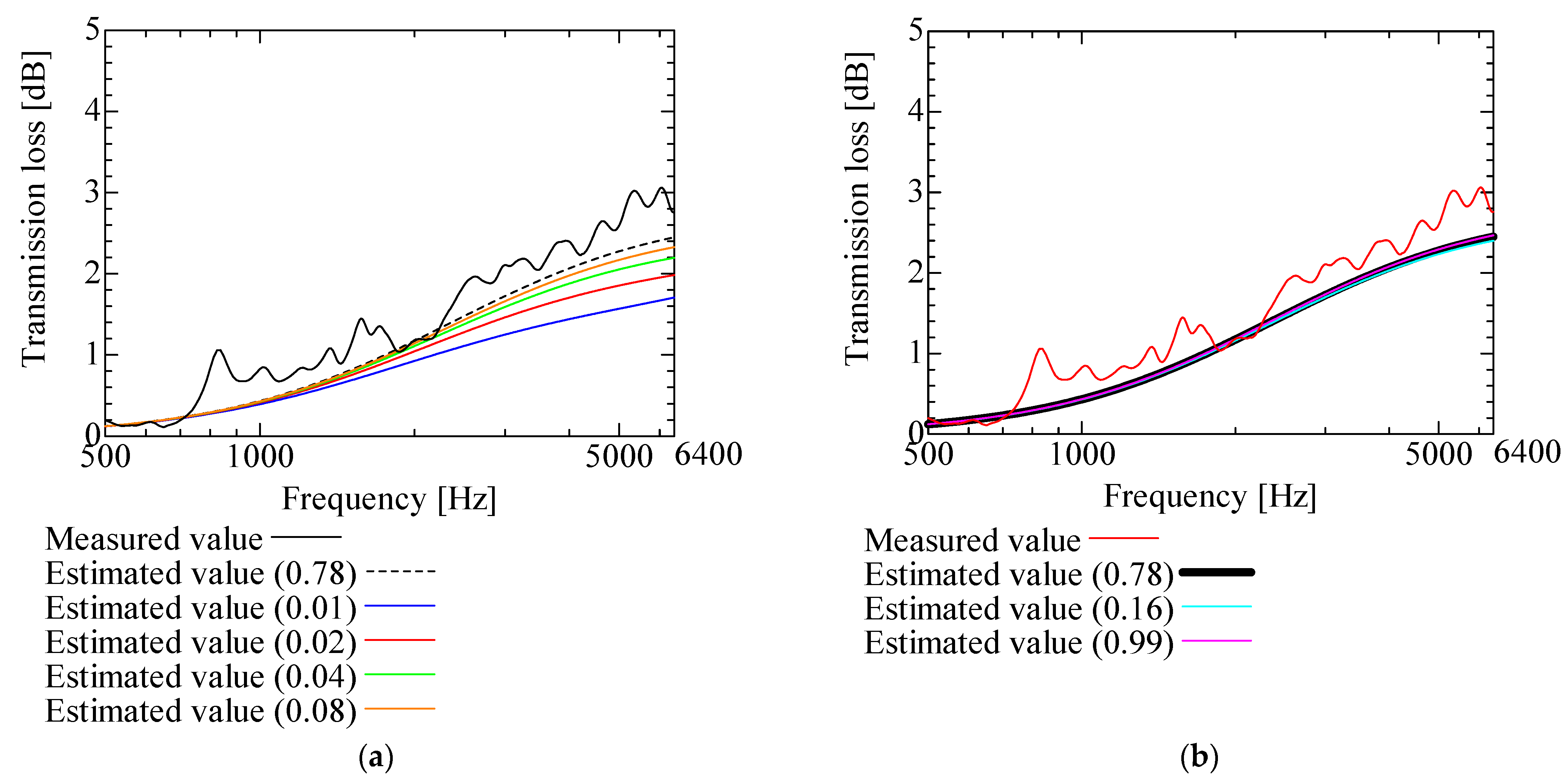
| Porosity | ϕ | 0.78 | ||
| Tortuosity | 1.1 | |||
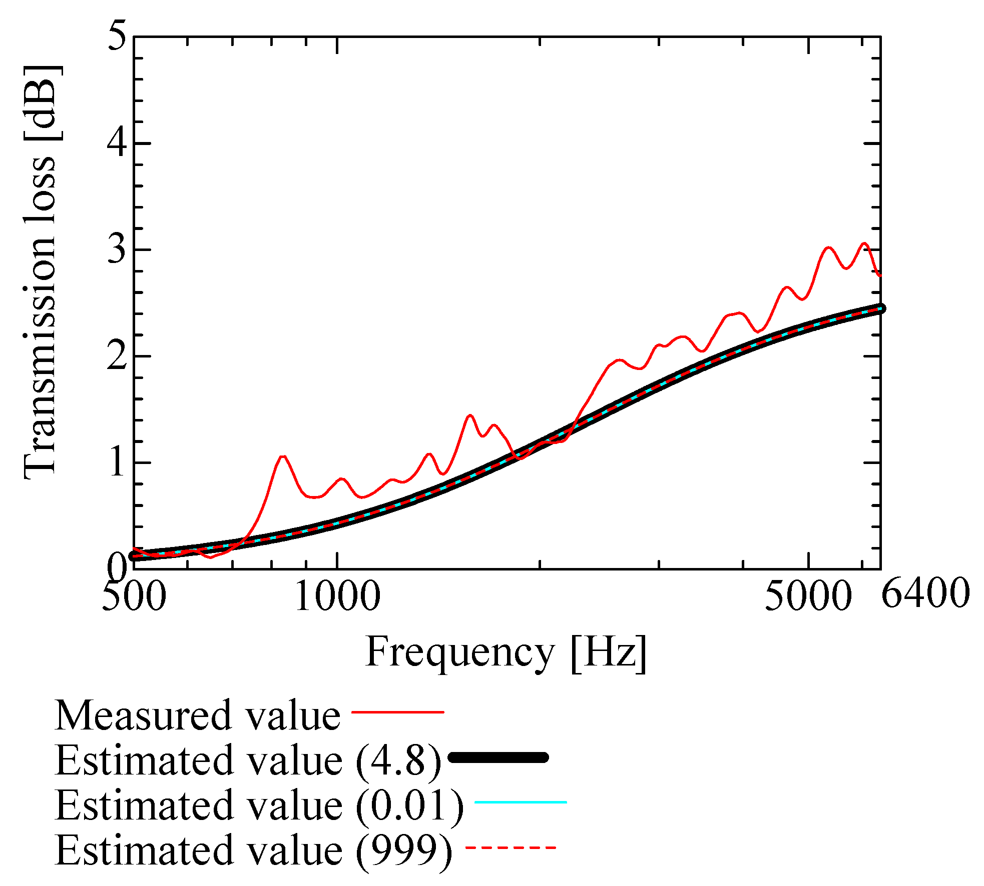
| Vicious characteristics length | 4.8 | µm | ||
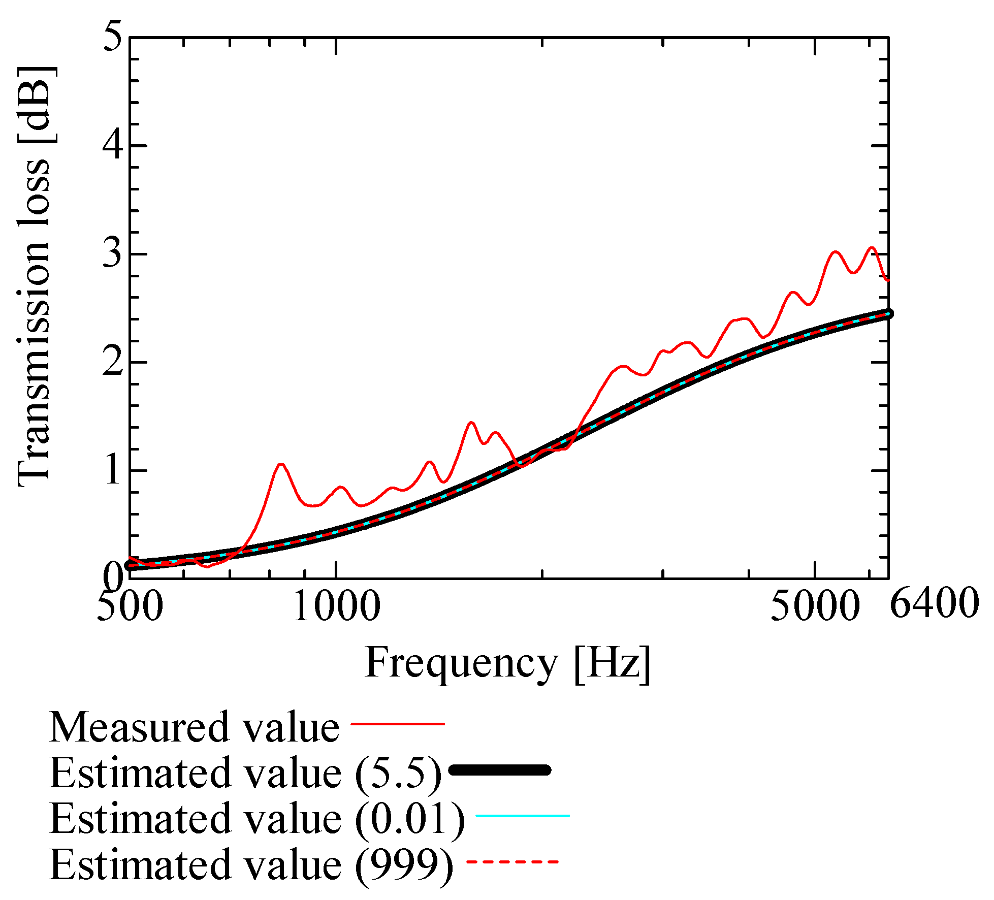
| Thermal characteristics length | 5.5 | µm | ||
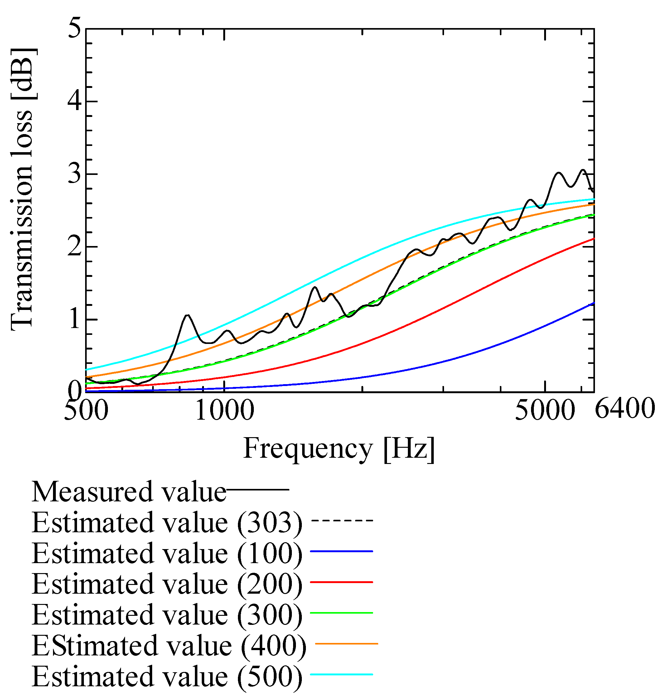
| Structual | Bulk density | 303 | kg/m3 |
Disclaimer/Publisher’s Note: The statements, opinions and data contained in all publications are solely those of the individual author(s) and contributor(s) and not of MDPI and/or the editor(s). MDPI and/or the editor(s) disclaim responsibility for any injury to people or property resulting from any ideas, methods, instructions or products referred to in the content. |
© 2023 by the authors. Licensee MDPI, Basel, Switzerland. This article is an open access article distributed under the terms and conditions of the Creative Commons Attribution (CC BY) license (https://creativecommons.org/licenses/by/4.0/).
Share and Cite
Sakamoto, S.; Hasegawa, T.; Ikeda, K. Estimation of Sound Transmission Loss in Nanofiber Nonwoven Fabrics: Comparison of Conventional Models and the Simplified Limp Frame Model. Nanomaterials 2023, 13, 2947. https://doi.org/10.3390/nano13222947
Sakamoto S, Hasegawa T, Ikeda K. Estimation of Sound Transmission Loss in Nanofiber Nonwoven Fabrics: Comparison of Conventional Models and the Simplified Limp Frame Model. Nanomaterials. 2023; 13(22):2947. https://doi.org/10.3390/nano13222947
Chicago/Turabian StyleSakamoto, Shuichi, Tsukasa Hasegawa, and Koki Ikeda. 2023. "Estimation of Sound Transmission Loss in Nanofiber Nonwoven Fabrics: Comparison of Conventional Models and the Simplified Limp Frame Model" Nanomaterials 13, no. 22: 2947. https://doi.org/10.3390/nano13222947