Entropy and Random Walk Trails Water Confinement and Non-Thermal Equilibrium in Photon-Induced Nanocavities

Abstract

Molecules near surfaces are regularly trapped in small cavitations. Molecular confinement, especially water confinement, shows intriguing and unexpected behavior including surface entropy adjustment; nevertheless, observations of entropic variation during molecular confinement are scarce. An experimental assessment of the correlation between surface strain and entropy during molecular confinement in tiny crevices is difficult because strain variances fall in the nanometer scale. In this work, entropic variations during water confinement in 2D nano/micro cavitations were observed. Experimental results and random walk simulations of water molecules inside different size nanocavitations show that the mean escaping time of molecular water from nanocavities largely deviates from the mean collision time of water molecules near surfaces, crafted by 157 nm vacuum ultraviolet laser light on polyacrylamide matrixes. The mean escape time distribution of a few molecules indicates a non-thermal equilibrium state inside the cavity. The time differentiation inside and outside nanocavities reveals an additional state of ordered arrangements between nanocavities and molecular water ensembles of fixed molecular length near the surface. The configured number of microstates correctly counts for the experimental surface entropy deviation during molecular water confinement. The methodology has the potential to identify confined water molecules in nanocavities with life science importance.

1. Introduction

Confined molecular water in nanocavities shows intriguing and unexpected behavior. The dynamic evolution of confined molecular water swings between bulk response, molecular collective actions and interface binding reactions [1]. Translational and rotational motions of confined water point to different stretching dynamics from its bulk counterpart [2]. It is also known that confined water builds tight hydrogen-bonded (H-bonded) networks, and its flow response is diverging by orders of magnitude from macroscopic hydrodynamics [3]. Possible lack of H-bonding of water molecules in small volumes counts for de-wetting, cavity expulsion [4], water self-dissociation [5] and a diverging dielectric constant [6]. It is plausible; therefore, that diverging behaviors of the biological and geological evolution of molecular enclosures in small systems [7,8,9,10,11,12,13] also imply a nanothermodynamic approach [14,15].

The central element of any thermodynamic theory of small systems is based on the hypothesis that nanometer-sized configurations pullout an additional physical component to the free energy of the associated macroscopic system from interactions among nanostructure entities. Moreover, the confinement of a relatively large number of molecules in nanocavities, restraints the molecular degrees of freedom (translational, vibration or rotational), and finally the system evolves through different entropic states before equilibration. 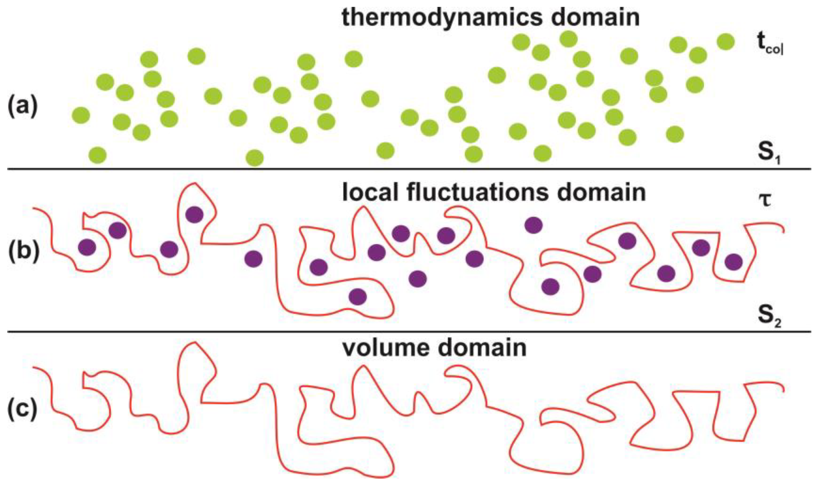Most interesting, the confinement of a small number of molecules in a large number of distinguishable tiny spaces might well indicate a thermodynamic entropic collective behavior [13], space and time local heterogeneities, not-extensive fluctuations and intriguing surface-boundary effects. The reduction of the translational degrees of freedom of molecules in tiny spaces and the deviation of the molecular trapping time inside a cavity from the mean molecular collision time outside, highlight the presence of an entropic barrier that separates the molecular motions inside and outside the cavities.

Today, both theoretical [14,15,16,17,18,19] and experimental advancements [20,21] gradually disclose the intriguing issues of thermodynamics of small systems, with major impacts on colloids, liquids, surfaces, interphases, chemical sensors, micro/nanofluidics, nanoporous media, proteins and DNA folding [10,22,23,24,25,26,27]. In cell biology, the presence of different nano-sized molecular scaffolds in the extracellular matrix environment implies a vast diversity of cellular activities and responses, including uncorrelated diverging drug delivery efficiencies [28].

Because thermodynamic potential variations and fluctuations allow for volume and surface stressing, any experimental verification of local volume and surface stress might well point to entropic fluctuations during molecular confinement [13,29]. Commonly, bulk and surface stressing go along with self-assembled structures, translational symmetry breaking, non-linearity, bifurcations, chaos, instability and morphological and shape nano configurations [30,31]. In the non-equilibrium state, rapidly changing thermodynamic potentials across phase boundaries usually force tiny systems to pass from different morphological progressions and physical states by tracing minimum energy and maximum entropy production pathways. This universal principle appears everywhere in Nature; from self-assembled bio and macromolecular structures and folding of large protein molecules [32] to nano/micro flower-like artificial structures [33,34].

The confinement of molecules within nano-size cavitations, usually on the surface of a matrix, is linked to system’s entropy diversity before and after trapping [13,27,35,36]. It is also known that for the same translational entropy, any confined molecular state attains a small variation of its rotational entropy compared to the non-confined molecular state. Likewise, rotational restriction affects surface molecular bonding and sorption/desorption kinetics [35]. Specific response of nanoentropic potentials from molecular confinement within photon-induced nanocavitations in PDMS matrixes underlines an inherent correlation between internal stressing and 2D entropy diversion [13].

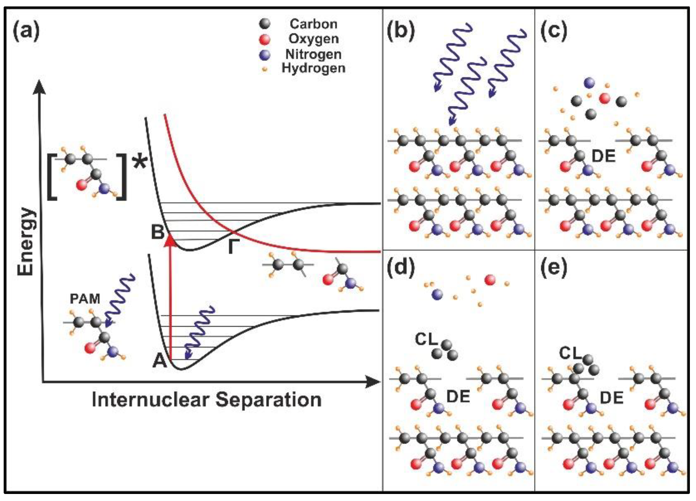
Commonly, photon-processing of surfaces reconfigures their physicochemical properties, including thermodynamic potentials [37,38,39,40]. Irradiation of a polymeric matrix with vacuum ultraviolet (VUV) light in the spectral range from 110 to 180 nm entails an extensive modification of topological and thus of physical features, because of bond breaking and formation of new bonds. Any 2D topological transform is accompanied by a diversion of surface characteristics, such as porosity, sensing efficiency, chemical stability and extensive nanocavitation [41,42,43,44,45,46]. The adsorption of various molecules on 2D nanostructured surfaces [47,48,49], might well boost a plethora of surfactant effects along with molecular sensing [43,50], gas separation and storage [51,52,53,54], and also applications with particular emphasis on nanomedicine [55], bio-engineering [56,57] and drug delivery systems [58,59]. Among other polymeric matrixes, polyacrylamide (PAM) is a hydrophilic low toxic, biocompatible, water-soluble, synthetic linear or cross-linked molecule, modified accordingly for a wide range of applications, including oil recuperation, wastewater treatment, soil conditioner, cosmetics food and biomedical industries [60,61,62]. A diverging number of physical and chemical methods are currently applied to optimize the biocompatibility level of different polymers (e.g., PDMS, PET, PTFEMA, PEG), for biomedical applications, biosensors, tissue engineering and artificial organs [46,63,64]. Well established methods of surface functionalization through photon irradiation with UV, VUV and EUV (extreme ultraviolet) light sources and plasma treatment at various wavelengths and electron energies, aim to optimize chemical instability and surface modification for controlling a plethora of surface functionalities [65].

Today, several methods exist to improve the strength and the physicochemical properties of PAM matrixes by blending the matrix with chitosan, starch or other polymers [66]. While functionalization of pure PAM polymeric surfaces is mostly done via sunlight exposure at standard environmental conditions, a limited number of studies include plasma processing [67,68,69,70,71]. However, no data exist for VUV processing of PAM surfaces, preventing thus precise tailoring of PAM’s physicochemical surface characteristics (surface roughness, structure size, elasticity, chemical composition, etc.) and the formation of controlled micro/nanopatterns and cavitations for different applications [37,42,43,63,64].

The current work establishes the link between entropy variation and molecular water confinement in small nanocavities fabricated by 157 nm laser photons in polymeric PAM matrixes. The work follows a line of a rational evolution. First, the correlation between 157 nm molecular photodissociation (laser fluence or a number of laser pulses) and surface topological features, including nanocavitations, is established from fractal and surface analysis by using atomic force microscopy (AFM). Next, the correlation between surface strain and 157 nm molecular photodissociation is revealed by applying AFM nanoindentation (AFM-NI), contact angle (CA) wetting and white light reflection spectroscopy (WLRS). Random walk simulations of water molecules inside cavitations differentiate the escape time of confined molecular water and the mean collision time of water molecules near the PAM surface. The different time scales inside and outside the nanocavities point to an additional state of ordered arrangements between nanocavities and the molecular water ensembles of fixed molecular length near the surface. The configured number of microstates properly counts for the experimental surface entropy deviation during molecular water confinement, in agreement with the experimental results. Finally, the mean time distribution for a small number of water molecules for different runs reveals a non-equilibrium state inside tiny cavities. The experimental method has the potential to identify confined water molecules in nanocavities via entropy variation. The proposed roadmap of analysis may be used in applications related to life science.

2. Materials and Methods

2.1. Materials

PAM (typical M_n = 150 K, M_w 400 K) purchased from Sigma-Aldrich (St. Louis, MO, USA) used to prepare solution 5% w/w in water. Thin layers (426 ± 1 nm) on Si wafer substrates were made by spin-coating for 60 s at 2500 rpm, and finally, cured at 110 °C for 15 min at a temperature rate of 0.37 °C s⁻¹ and then left to cool at room temperature. WLRS measures the thickness of PAM films coated on Si wafers.

2.2. 157 nm Laser

PAM layers irradiated with a high power pulse discharged molecular fluorine laser at 157 nm (Lambda Physik 250 (LPF^TM 200), Lambda Physik AG (Coherent), Göttingen, Germany), under continuous nitrogen flow (99.999%) at 10⁵ Pa and room temperature. The layers were mounted into a computer-controlled X-Y-Z-θ translation-rotation motorized stage, placed inside a 316 stainless-steel chamber. The laser temporal pulse duration at FWHM, the energy of an unfocused laser beam per laser pulse, the photon fluence per laser pulse and laser repetition rate were set up at 15 ns, 28 mJ, 250 Jm⁻² and 10 Hz. For dipping the amount of oxygen inside the stainless-steel chamber, nitrogen purging of the chamber was applied for 10 min before the irradiating stage.

2.3. AFM Imaging and AFM-NI

An AFM system (diInnova, Veeco Instruments Inc. (SPM Bruker), Santa Barbara, CA, USA) used for surface imaging of exposed/non exposed areas and the AFM-NI measurements. The imaging carried out in a tapping mode at a scanning rate of 0.5 Hz, using phosphorus-(n)-doped silicon cantilever (MPP-11123-10), having a spring constant of 40 nN nm⁻¹ and tip radius of 8 nm, operating at a resonance frequency of 300 kHz at ambient conditions. The surface parameters of the samples were also evaluated.

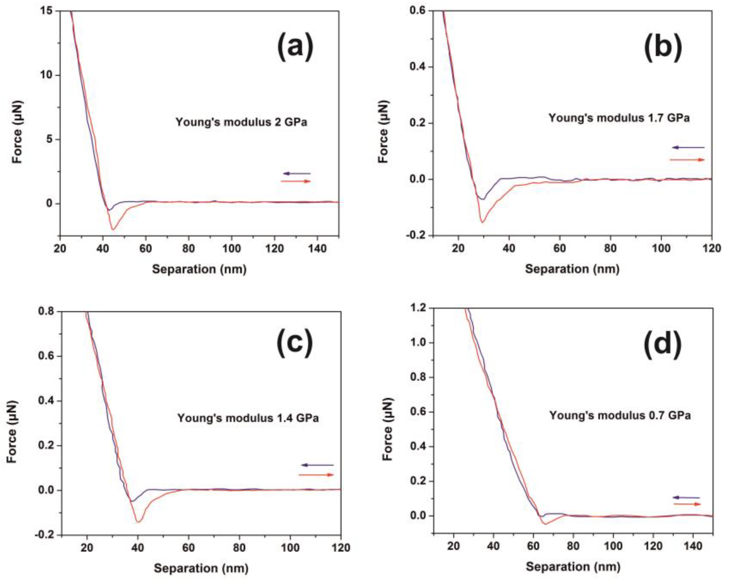
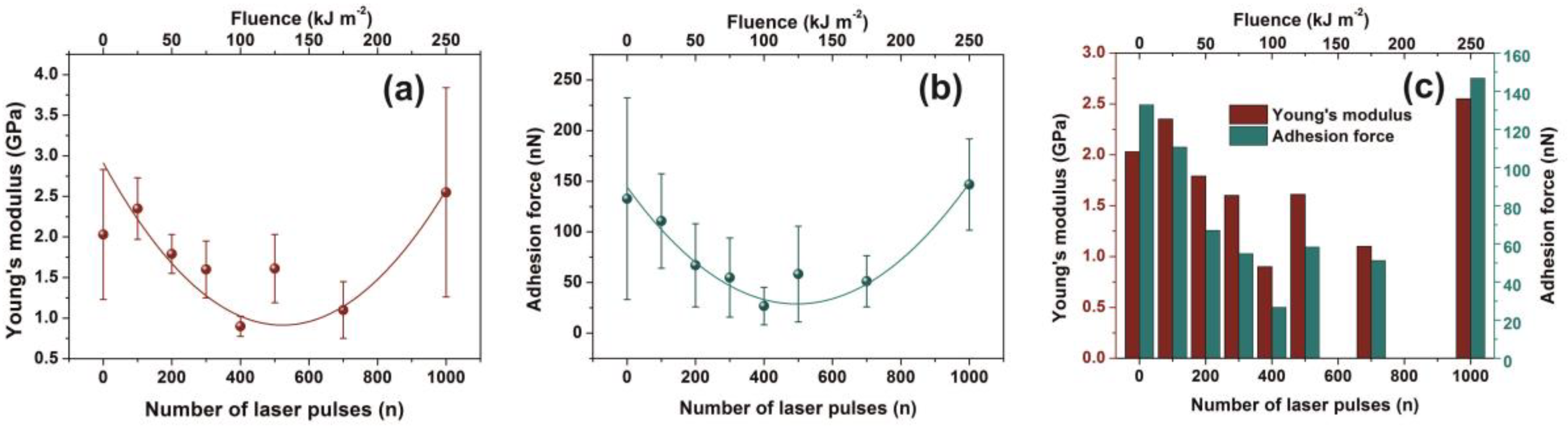
The force versus distance (F-D) response from ten different points on each non-exposed and exposed areas was also recorded with the same cantilever. The elastic modulus (Young’s modulus) was calculated using the SPIP force curve analysis software by fitting a Hertz model to the force-distance curve. The hysteresis between approach and retract curves were corrected by the same software. Calculations performed with a Poisson’s ratio value of 0.3 [72].

2.4. Fractal Analysis

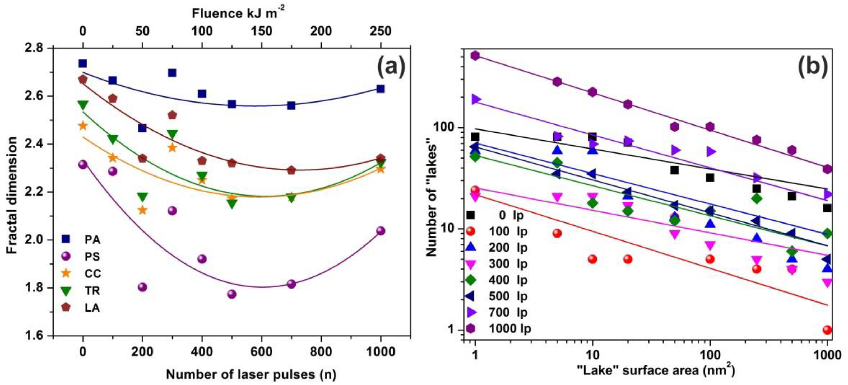
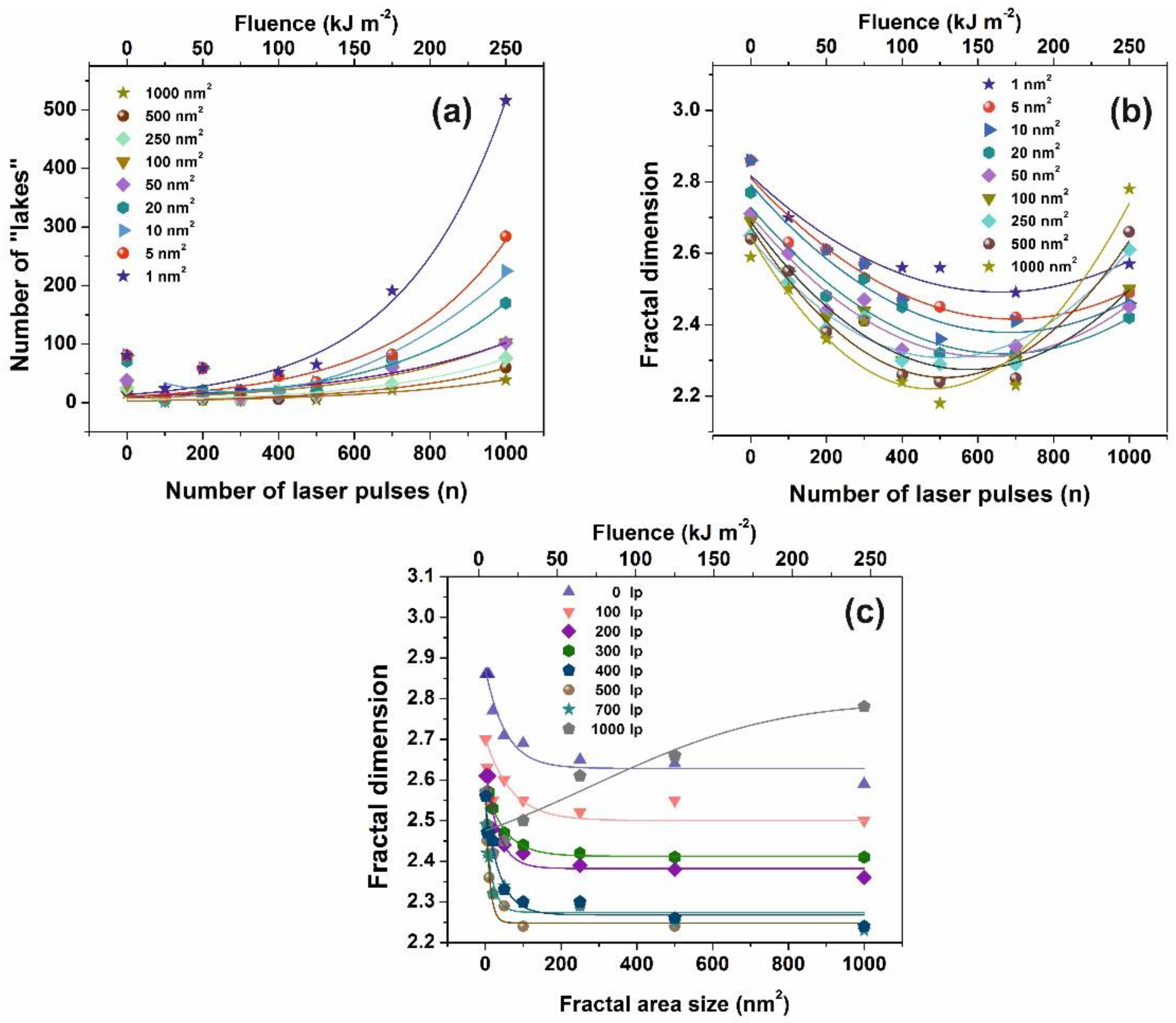
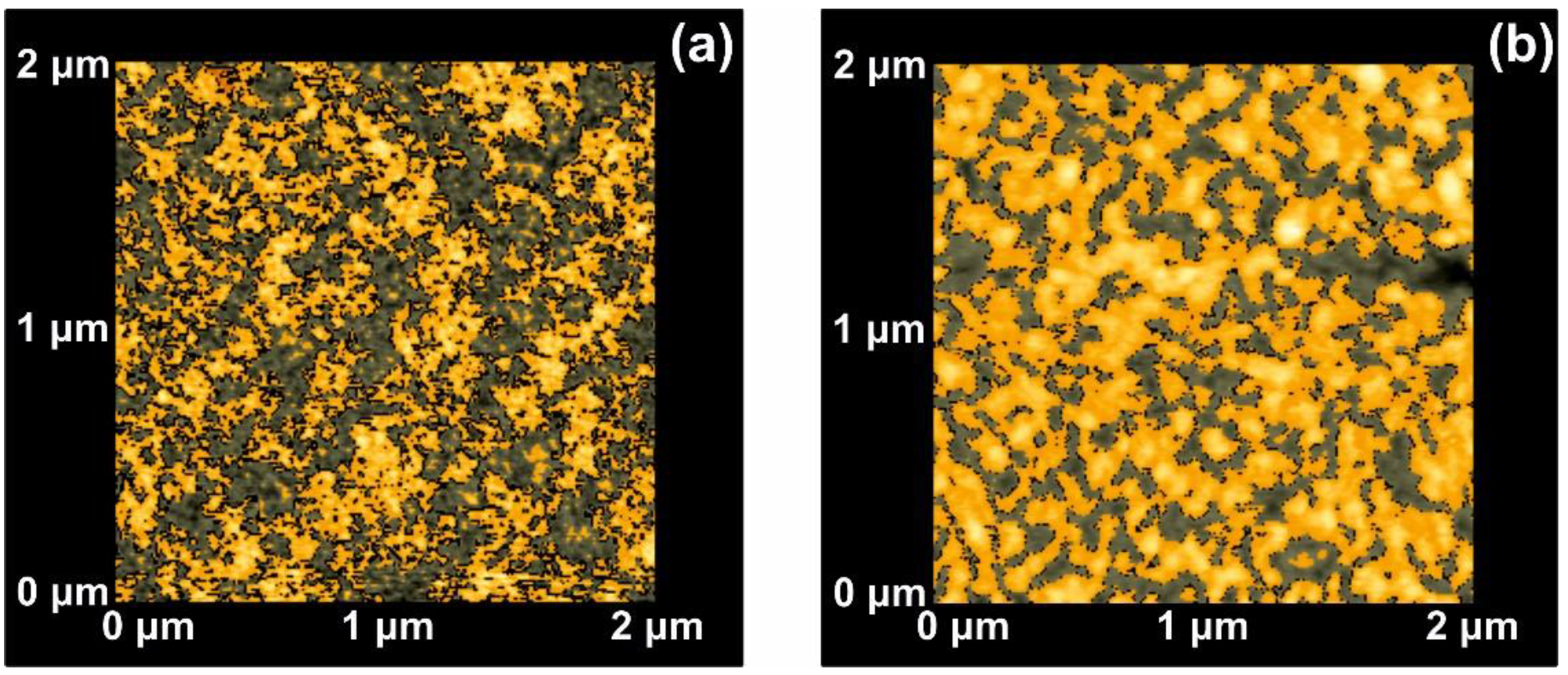
The fractal characteristics of the exposed and non-exposed areas were quantified through the fractal dimensionality D_f that describes the topology and the cavitation of a surface quantitatively. D_f was derived from AFM images by four different algorithms, the cube counting, triangulation, variance and power spectrum methods, besides an algorithm provided by the AFM’s “lake pattern” software (diSPMLab Vr.5.01). A detailed description of the concept and the specific methodologies of the different algorithms can be found in [27]. The D_f was calculated for the four different methods using “Gwyddion, SPM data visualisation and analysis tool” [73]. The D_f calculated with the four different algorithms follow the same trend, despite small dimensionality divergences coming up from systematic errors, because of the different converging speed of the fractal analytical approaches.

2.5. Water Contact Angle (CA)

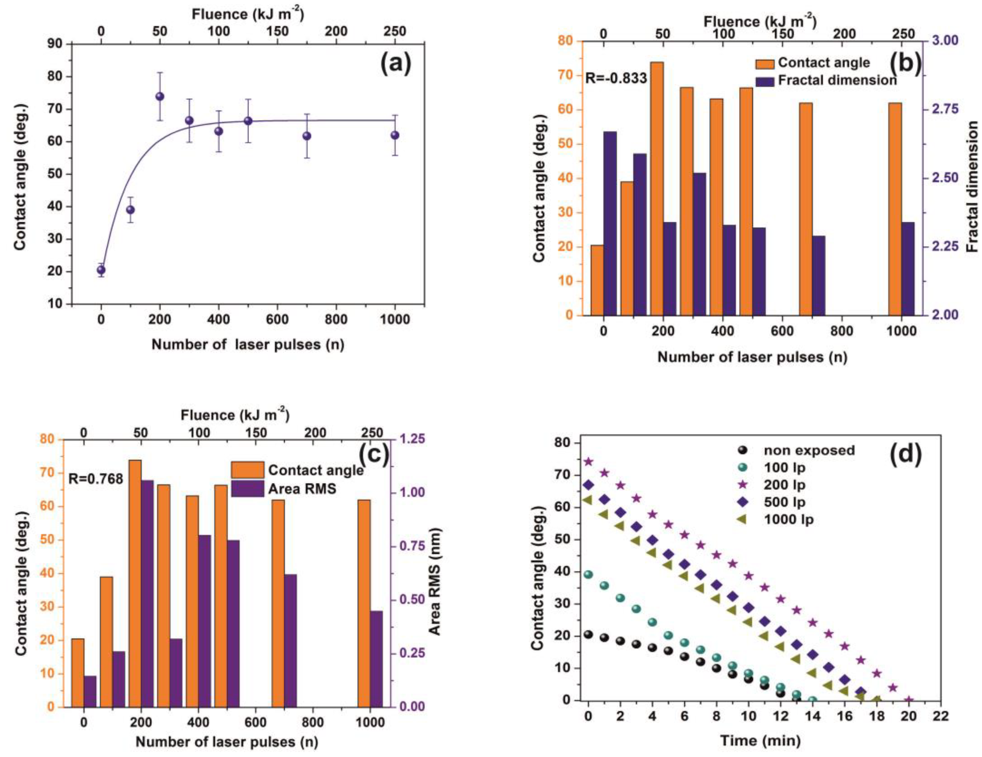
The chemical modification of PAM surfaces following PAM surface laser irradiation was monitored by water CA surface measurements under ambient atmospheric conditions. Distilled water droplets with a volume of 0.5 μL were gently deposited onto the sample surface using a microsyringe. Water CAs on samples before and after irradiation and at different time intervals were measured using a CA measurement system (Digidrop, GBX, Romans sur Isere, Drôme, France) equipped with a CCD camera to capture lateral snapshots of a droplet deposited on top of the preselected area, suitable for both static and dynamic CA measurements. Droplet images captured at a speed of 50 frames/s. CA values were obtained via the Digidrop software analysis, approximating the tangent of the drop profile at the triple point (three-phase contact point). Three different CA measurements were taken from each sample at different sample positions to calculate the average values.

2.6. White Light Reflectance Spectroscopy (WLRS)

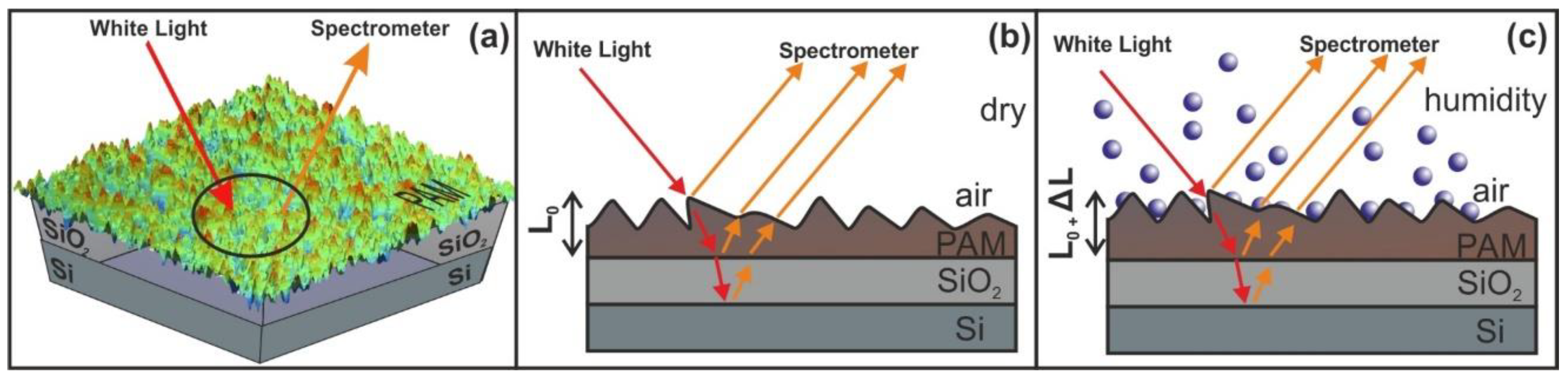
The WLRS measurements were performed by an FR-Basic, ThetaMetrisis™ (ThetaMetrisis SA, Athens, Greece) equipped with a VIS–NIR spectrometer (Theta Metrisis SA, Athens, Greece) having 2048 pixels detector and optical resolution of 0.35 nm. The beam of the light source comes from a white light halogen lamp, with a uniquely designed stable power supply and soft-start circuit, ensuring stable operation over time that is necessary for long time duration experiments. Software controls the instrument, performing the data acquisition and film thickness calculations. The PAM films were spin-coated on native oxide Si wafers and SiO₂ layer on the top with a thickness of 2–3 nm.

2.7. Random Walk Model

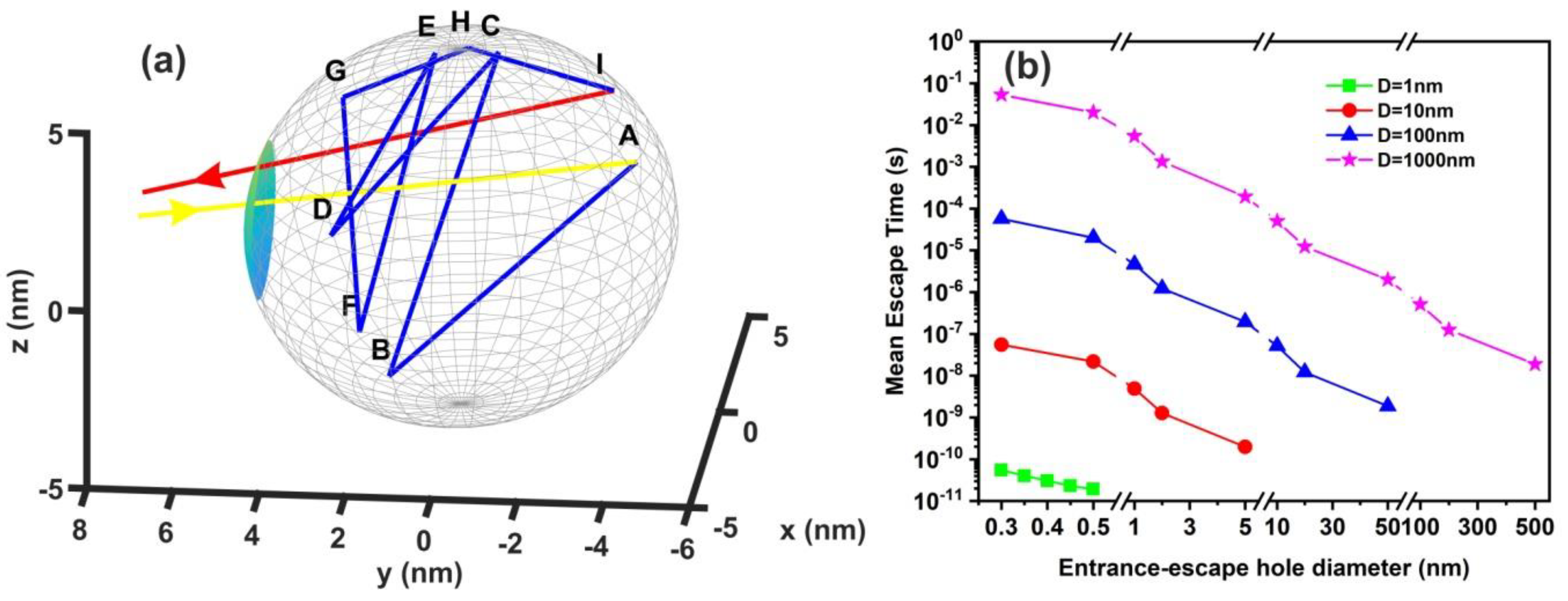
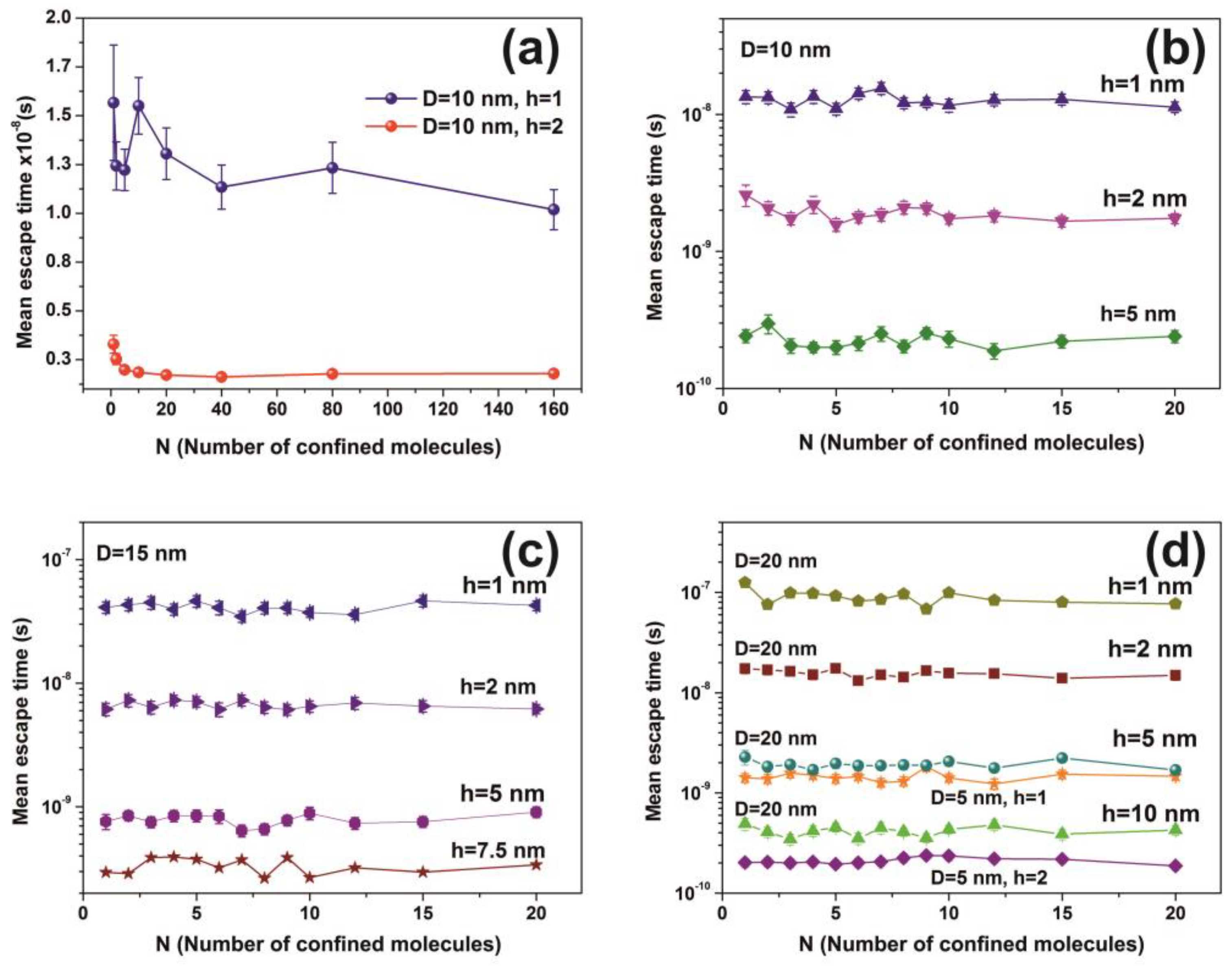
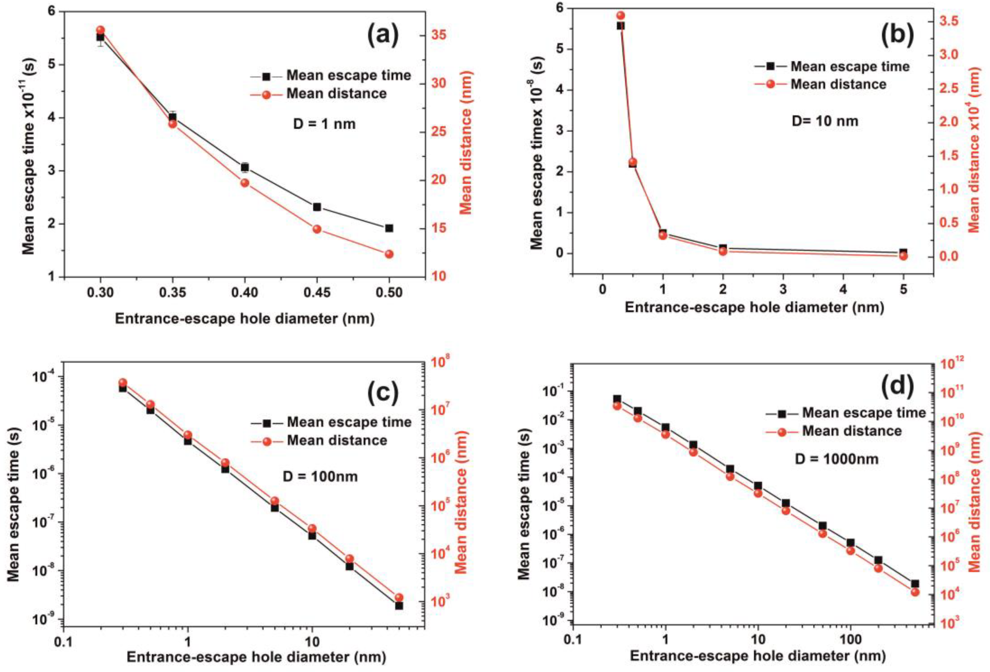
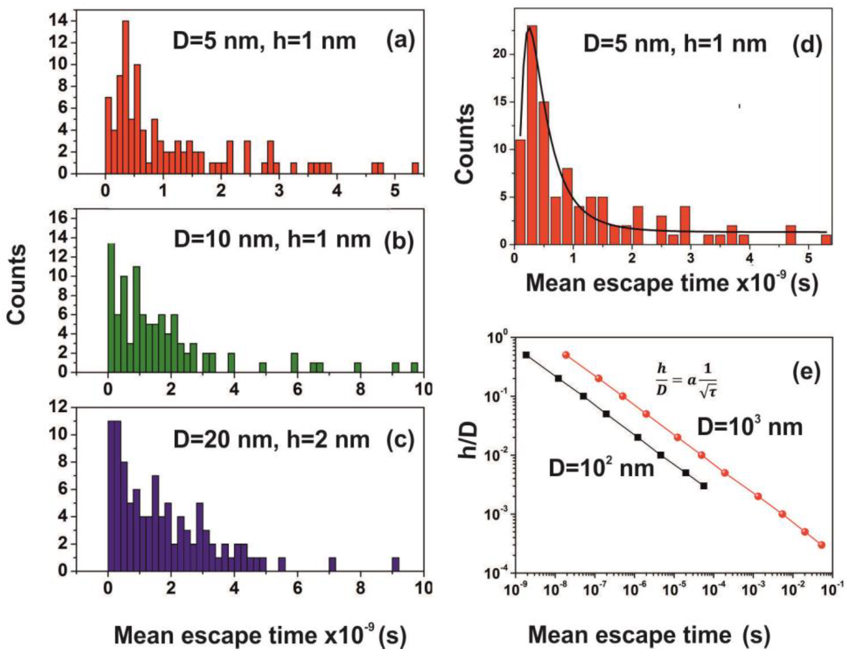
The mean escape time of a water molecule confined in nanocavities was computed by applying different 3D random walk models with diverging numbers of water molecules, variable spherical size nanocavities, and entrance-escape hole sizes. Two different models of non-interactive and interactive water molecules inside the cavities were used. The first model, the non-interactive random walk model, uses molecular masses of zero volume and elastic collisions of the water molecule with the cavity wall and it records the sequence of positions of water molecules inside the spherical cavity until it gets back to the entrance-escape hole. The collision angle was varied randomly with a uniform distribution. The model calculates the total distance that molecules travel in the cavity before they escape from the entrance-escape hole. The mean escape time was calculated by considering that the molecule attains its kinetic energy after an elastic collision with the walls of the cavity. Therefore the kinetic energy transfer from the wall to the molecule should be equal with the thermal energy of the wall $\frac{3}{2}{k}_{B}T$, where $k_B$ is Boltzmann’s constant.

The escape time from the entrance-escape hole for a non-interactive water molecule in the cavity is given by the equation:

$$t_e=\frac{{{\displaystyle \sum }}_{i=0}^n\left(\sqrt{2R^2(1-\sin {\theta }_{i+1}\sin {\theta }_i\cos \left({\phi }_{i+1}-{\phi }_i\right)+\cos {\theta }_{i+1}\cos {\theta }_i} \right)-2R+\left(R_0+R_n\right)}{\sqrt{\frac{3k_{B}T{N}_A}{M_{H_{2}O}}}}$$

(1)

where n is the number of collisions in each run, R is the radius of the spherical cavity, $\left(R,{\theta }_i,{\phi }_i\right)$ is the position of the molecule in the ith collision. The entrance and the exit point in the cavity wall are given in spherical coordinates $\left(R_0,{\theta }_0,{\phi }_o\right)$ and $\left(R_0,{\theta }_n,{\phi }_n\right)$, accordingly, and $M_{H_{2}O}$ is the molecular mass of water.

The interactive random walk model records the sequence of positions of a specific molecule that enters a spherical cavity through the entrance-escape hole, alongside with the locations of a variable number of neighboring molecules trapped in the cavity, until it gets back to the entrance-escape hole. At first, because of non-thermal equilibrium between water molecules within the cavity, the molecules are placed inside the cavity in random positions with random velocities of uniform distribution between 0 and $\sqrt{\frac{3k_{B}T{N}_A}{M_{H_{2}O}}} \mathrm{m}/\mathrm{s}$. The position of each molecule was recorded every${10}^{-14}\mathrm{s}$. The collision of each water molecule with the cavity wall and its neighbouring molecules is considered to be elastic. The collision angle was varied randomly with a uniform distribution. Contrary to the non-interactive model of zero-size molecules, the interactive model uses a spherical molecular diameter of 0.3 nm.

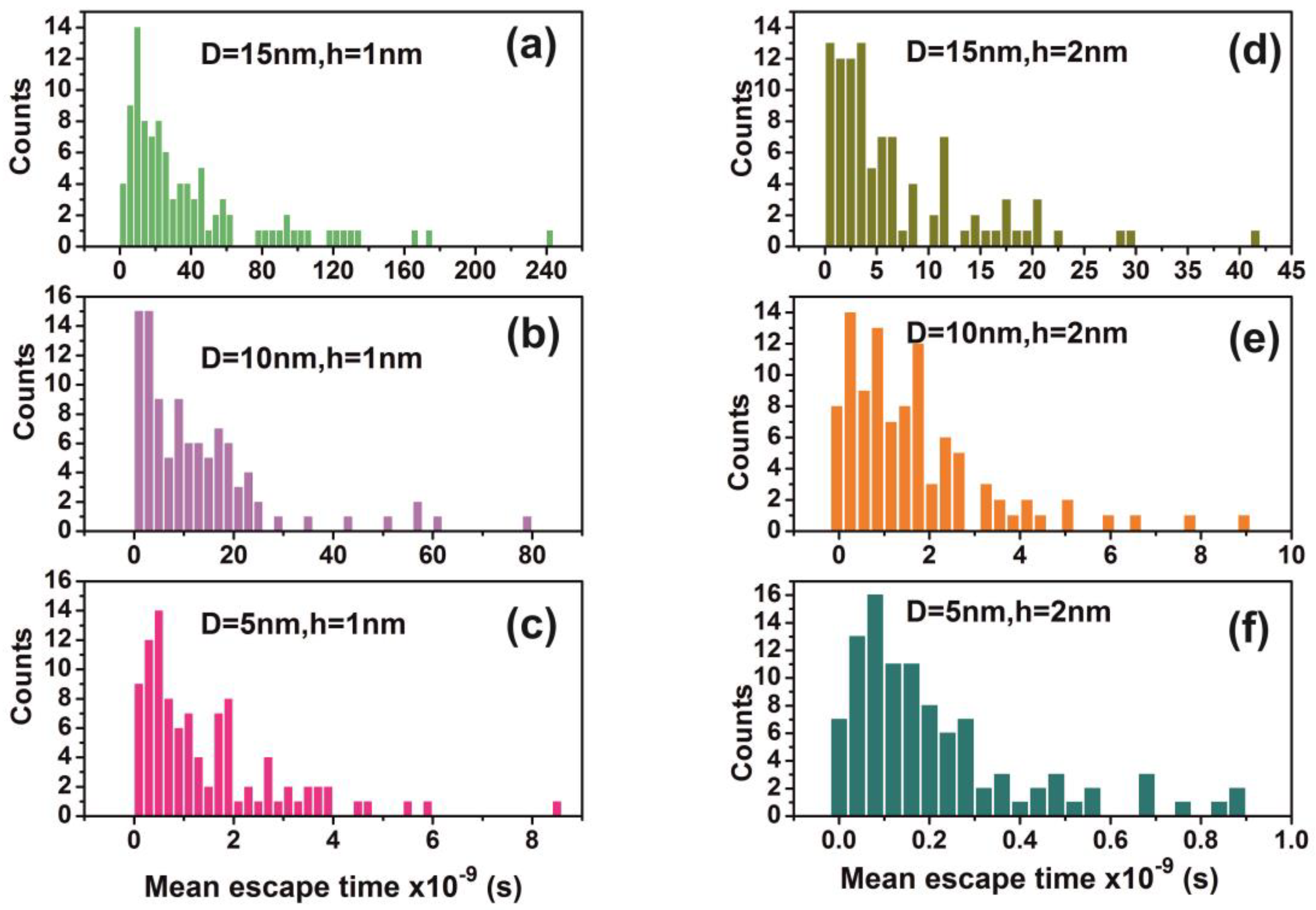
For every pair of the cavity size and entrance-escape hole, the random walk was run 10² times and the mean escape time was calculated. In addition, the mean-escape time distribution for different cavities and number of molecules was used to evaluate the thermodynamic state inside the cavity. The model was designed and run in MATLAB. 9.4.0.813654 (R2018a), The MathWorks Inc.; Natick, MA, USA.

3. Results

3.1. Surface Analysis

Commonly, four surface parameters, the surface roughness histogram, the area roughness, the area root mean square (RMS) and the maximum range characterize a surface and mean area values are plotted as functions of the laser pulse number or the laser fluence, Figure 1. The surface parameters are extracted from AFM images, Figure 2a–e.

The surface roughness histogram, or average z-height, is the arithmetic mean defined as the sum of all height values divided by the number of data points $\left|Z\right|=\frac{1}{N}\sum _{i=1}^N{Z}_i$. Next, the R_a (area roughness or roughness average) is the arithmetic mean of the height deviation from the image’s mean value,$R_a=\frac{1}{n}\sum _{i=1}^n\left|Z^i-\overline{Z}\right|$. The area RMS (R_rms) is the value defined as the square root of the mean value of the squares of the distance of the points from the image mean value: $R_{rms}=\sqrt{\frac{1}{N}\sum _{i=1}^N{\left(Z-Z_i\right)}^2}$. Finally, the maximum range of Z_max is defined as the maximum value of z-heights. The surface parameter values (z-height, area roughness, area RMS, and maximum range) of photon exposed areas were more considerable compared to the non-irradiated ones. However, because surface parameters are area size-dependent (Figure 2d,e), they are utilized only for a comparative qualitative evaluation of area modification under 157 nm laser irradiation.

3.2. Fractal Analysis of 157 nm Photon Processed PAM Polymeric Matrixes

Because of statistical self-similarity between matrix space topology during a scaling-down route, there is a strong correlation between porosity, stage of cavitations and fractal dimensionality. Furthermore, in porous materials, the linear, area and volumetric porosities are alike, and therefore the 3D fractal dimensionality is similar to the area one. The dimensionality of a surface is equal to two for an ideal solid (Euclidean surfaces) and equal to three for completely porous surfaces with a fractal character. Areas with Z_i values above a threshold Z height are known as “islands”, while those with Z_i’s below the threshold height value are named as “lakes”. AFM “island-lake structure” of non-irradiated and VUV irradiated 2 μm × 2 μm areas are shown in Figure 3.

The mean Z_i heights of non-irradiated and the irradiated regions (10³ laser pulses) were set at 0.75 and 1.94 nm respectively, and the irradiated areas show a diverging surface topology, in agreement with previous results [13,16,56,58]. Following a standard procedure, two parameters, the fractal dimensionality D_f (which is a dimensionless number) and the “periphery to the area ratio” (PAR) are used to describe a set of “islands” or “lakes”. Both parameters are linked to the surface roughness, cavitations and topological entropy [27,74]. PAR is the ratio of logarithms of the perimeter Π to the area A, where $\Pi =\alpha \left(1+D_f\right)A^{\left(1-D_f\right)/2}$. For assessing the state of cavitations, the fractal dimensionality is calculated by the partitioning, the cube counting, the triangulation, and the power spectrum algorithms [58]. Results are compared with those derived directly from the AFM “lake” pattern software, Figure 4a.

AFM images of 2 μm × 2 μm laser-irradiated areas were digitized to a 512 px × 512 px matrix, and then they processed with four different fractal algorithms. It is unveiled that fractal dimensionality, and thus cavitations, are functions of the laser photon fluence. All algorithms exhibit a similar trend of fractal dimensionality with the number of laser pulses (laser fluence), although the fractal dimensionality derived with the power spectra methodology seems slightly different, as expected [13,25]. The fractal dimensionality initially dips, attaining its minimum value around 500 laser pulses and then rises again with a small gradient up to 10³ laser pulses, Figure 4a. For a constant “lake” surface area the number of “lakes”, and thus the number of cavities, is a function of the laser pulses (laser fluence), Figure 4b. The number of “lakes” within a given surface area vs. the number of laser pulses is shown in Figure 5a. The number of “lake” areas rises almost exponentially with the number of laser pulses and small area “lakes” prevail over larger ones The fractal dimensionality vs. laser fluence has a non-monotonous complex structure. Small size features (1–10² nm²) are associated with nanocavity-like structures, Figure 5b. It is also confirmed that below 10³ laser pulses small size features contribute to a high cavitation state because small size features have a higher dimensionality than large size structures, Figure 5c. On the contrary, large size features are prominent at 10³ laser pulses, indicating the complexity of the associated processes. In addition, for the same number of laser pulses, small size cavitation prevails over larger ones, Figure 5a. The experimental results indicate that water confinement is rather associated with small cavitations, in agreement with WLRS measurements (vide infra).

3.3. AFM-NI

The mechanical response of 426 nm-thick PAM polymers was evaluated with nanoscale resolution via the F-D curves at different laser fluence, Figure 6a–d. Young’s modulus and adhesion forces were also evaluated. Major non-monotonic modifications were recorded indicating substantial conformational changes of the surface energy of the PAM layers, Figure 6a. A diverging Young’s modulus is attributed to accelerated ageing because of molecular bond breaks, accompanied by the formation of new carbon and carbonyl bonds [75,76,77]. A nonlinear alteration of the elastic modulus of PAM gel formulations during ten days ageing was also reported, revealing substantial changes of PAM’s mechanical properties during irradiation [78].

The approach and retract curves follow different paths in all irradiating conditions, describing thus a system evolving out of equilibrium. The elastic modulus of the dry state hydrogels is significantly reduced after immersion to water, e.g., from 18 GPa to 3.3 MPa [79]. The Young’s modulus of the non-irradiated PAM hydrogels depends on the hydration conditions, e.g., it decreases from 295 MPa in the dried state to 266 kPa in the fully hydrated state [78,80]. A Young’s modulus of 2.84 GPa of uncured PAM hydrogel was recently attributed to the presence of pre-polymerized PAM oligomers [81]. Moreover, enhancement of Young’s modulus to 4.84 GPa was predicted via an extension of the 3D polymeric networks at higher cross-linking states [81].

In this work, the non-irradiated PAM surfaces were thermally cured after being spin-coated on a silicon wafer; therefore, their mechanical properties are expected to deviate from those in the gel state. The average Young’s modulus prior to and post-irradiation with 500 and 10³ laser pulses was 2.0 ± 0.8 and 1.6 ± 0.42 and 2.55 ± 1.29 GPa, respectively, Figure 7a. The significant errors of Young’s moduli at different points in the same sample are credited to various morphological heterogeneities and a progressive phase transformation to a relatively high carbonized state. Young’s moduli follow a similar trend with fractal dimensionality vs. laser fluence, Figure 4a and Figure 5b.

Additionally, the adhesive force, as it is measured during the penetrating state of AFM’s tip, follows a similar trend with Young’s modulus, Figure 7b,c. Because of diverging surface carbonization, the adhesive force drops from 130 to 26 nN between 0–400 laser pulses and then it rises again to ~ 150 nN for 10³ laser pulses.

3.4. Water Contact Angle (CA)

Water CAs of PAM matrixes were recorded for varying photon fluence. The average CAs rise from 20° ± 2° to a saturated “plateau” at ~65°± 7° after 200 laser pulses, Figure 8a.

VUV photon processed PAM matrixes attain higher CA values, displaying thus a hydrophobic state, affirming that VUV irradiation has a primary effect on the surface wettability by altering both the material’s physicochemical properties and surface nano/micro features, Figure 8a,b. In addition, the mean correlation factors of −0.833 and 0.768 between CA, D_f and area RMS indicate a secure interconnection between surface morphology and D_f, Figure 8b,c.

The wetting behavior was also analyzed with time, Figure 8d. The CAs of non-irradiated and irradiated with 100 laser pulses matrixes decrease consistently for 5 min. The dynamic CA of irradiated samples exhibits similar slope values, suggesting similar diffusion constants for different porosities, a fact that stresses out a picture of molecular water confinement in nanocavitations.

3.5. White Light Reflectance Spectroscopy (WLRS)

WLRS uses a broad-band light source and a spectrometer. The white light emitted from the light source is guided to a reflection probe through a number of optical fibers that incident vertically onto a sample. The sample consists of a stack of transparent and semi-transparent films placed over a reflective substrate. A reflection probe collects the reflected light through a fiber, directing it to the spectrometer. The light source beam interacts with the sample and generates a reflectance signal that is constantly recorded by the spectrometer. The number and the shape of interference fringes, registered in the CCD of the spectrometer, depend on the thickness and the refractive index of the film(s). The fitting of the experimental spectrum is performed by using the Levenberg-Marquardt algorithm.

Water confinement is a source of volume strain and the relative surface deformation of the PAM polymeric matrixes caused by molecular water confinement is monitored by WLRS, Figure 9. The layer’s thickness during water confinement and the relative surface deformation of the PAM layer prior and after water confinement in the irradiated surfaces is calculated from the phase shift and the superposition of amplitudes of the reflected light beam on the PAM surfaces. The white light beam records the surface strain within a cylindrical volume ~ V = 4.09 × 10⁻¹⁴ m³, defined by the cross-sectional diameter of the white light beam of 3.5 × 10⁻⁴ m and the thickness of the polymeric layer of 426 nm.

3.6. Random Walk Model

The comparison between calculations with the diffusion model [82] (water vapour diffusion coefficient in the air at normal pressure at 293 K is ~ 2.42 × 10⁻⁵ m² s⁻¹) and the current non-interactive random walk model for 10³ runs is shown in

Table A1. Mean escape time (τ) of a given molecule, errors and total traveling distance of the confined molecule in a spherical cavity (cavity diameter D of 1 nm and 10 nm) for different entrance–escape hole diameters (h) calculated by the diffusion and the non-interactive random walk models.

h (nm)	Cavity Diameter D = 1 nm					Cavity Diameter D = 10 nm
	Diffusion	Random Walk				Diffusion	Random Walk
	τ (s)	τ (s)	Error (s)	Distance (nm)	Error (nm)	τ(s)	τ (s)	Error (s)	Distance (nm)	Error (nm)
0.3	3.98 × 10−14	5.51 × 10−11	1.7 × 10−12	35.5	1.1	3.98 × 10−11	5.57 × 10−8	1.7 × 10−9	35,931	1133
0.5	2.39 × 10−14	1.91 × 10−11	5 × 10−13	12.4	0.3	2.39 × 10-11	2.19 × 10−8	7 × 10−10	14,151	465
1						1.19 × 10-11	4.93 × 10−9	1.6 × 10−10	3182	107
2						5.98 × 10-12	1.28 × 10−9	4 × 10−11	822	26
5						2.39 × 10−12	1.90 × 10−10	5 × 10−12	128	4

and

Table A2. Mean escape time (τ) of a given molecule, errors and total traveling distance of the confined molecule in a spherical cavity (cavity diameter 10² nm and 10³ nm) for different entrance–escape hole diameters (h) calculated by the diffusion and the non-interactive random walk models.

h (nm)	Cavity Diameter D = 102 nm					Cavity Diameter D = 103 nm
	Diffusion	Random Walk				Diffusion	Random Walk
	τ (s)	τ (s)	Error (s)	Distance (nm)	Error (nm)	τ (s)	τ (s)	Error (s)	Distance (nm)	Error (nm)
0.3	3.98 × 10−8	5.71 × 10−5	1.8 × 10−6	3.68 × 107	1.2 × 106	3.98 × 10−5	5.3 × 10−2	1.7 × 10−3	3.42 × 1010	1.1 × 109
0.5	2.39 × 10−8	2.00 × 10−5	6 × 10−7	1.29 × 107	4.1 × 105	2.39 × 10−5	2.01 × 10−2	6.3 × 10−4	1.3 × 1010	4.1 × 108
1	1.19 × 10−8	4.63 × 10−6	1.4 × 10−7	2.99 × 106	9 × 104	1.19 × 10−5	5.43 × 10−3	1.6 × 10−4	3.5 × 109	1.1 × 108
2	5.98 × 10−9	1.22 × 10−6	4 × 10−8	7.89 × 105	2.5 × 104	5.98 × 10−6	1.33 × 10−3	4.1 × 10−5	8.56 × 108	2.7 × 107
5	2.39 × 10−9	1.95 × 10−7	6 × 10−9	1.26 × 105	4 × 103	2.39 × 10−6	1.92 × 10−4	6.7 × 10−6	1.24 × 108	4.3 × 106
10	1.19 × 10−9	5.18 × 10−8	1.6 × 10−9	3.34 × 104	1060	1.19 × 10−6	4.99 × 10−5	1.6 × 10−6	3.22 × 107	1.1 × 106
20	5.97 × 10−10	1.21 × 10−8	3 × 10−10	7821	244	5.97 × 10−7	1.23 × 10−5	4.1 × 10−7	7.93 × 107	2.6 × 105
50	2.39 × 10−10	1.87 × 10−9	5 × 10−11	1204	35	2.39 × 10−7	1.99 × 10−6	6.4 × 10−8	1.28 × 106	4.1 × 104
100						1.19 × 10−7	5.07 × 10−7	1.5 × 10−8	3.27 × 105	9.8 × 103
200						5.97 × 10−8	1.25 × 10−7	3.7 × 10−9	8.05 × 104	2.4 × 103
500						2.39 × 10−8	1.88 × 10−8	5.6 × 10−10	1.21 × 104	3.6 × 102

. There is a noticeable difference between the two models for small size nanocavities because the diffusion constant for small size nanocavities is undetermined. The mean escape time from random walk models with the interactive model for the different number of confined molecules, cavity and the entrance-escape hole size is given in Figure 10 and Appendix A,

Table A3. Mean escape time (τ) and associated errors of different number molecules confined in a 5-nm spherical cavity for different entrance–escape hole diameters (h) calculated by the interactive random walk models for 10² runs.

Cavity Diameter = 5 nm
N (Number of Molecules)	h = 1 nm		h = 2 nm
	τ (s)	Error (s)	τ (s)	Error (s)
1	1.41 × 10−9	1.4 × 10−10	2.02 × 10−10	2.0 × 10−11
2	1.38 × 10−9	1.4 × 10−10	2.04 × 10−10	2.2 × 10−11
3	1.57 × 10−9	1.6 × 10−10	2.00 × 10−10	2.1 × 10−11
4	1.50 × 10−9	1.4 × 10−10	2.05 × 10−10	1.9 × 10−11
5	1.39 × 10−9	1.4 × 10−10	1.95 × 10−10	1.8 × 10−11
6	1.46 × 10−9	1.3 × 10−10	2.01 × 10−10	2.2 × 10−11
7	1.27 × 10−9	1.2 × 10−10	2.06 × 10−10	2.1 × 10−11
8	1.30 × 10−9	1.4 × 10−10	2.25 × 10−10	2.4 × 10−11
9	1.82 × 10−9	1.8 × 10−10	2.37 × 10−10	2.1 × 10−11
10	1.41 × 10−9	1.4 × 10−10	2.35 × 10−10	2.4 × 10−11
12	1.23 × 10−9	1.5 × 10−10	2.20 × 10−10	2.1 × 10−11
15	1.53 × 10−9	1.5 × 10−10	2.18 × 10−10	2.0 × 10−11
20	1.47 × 10−9	1.3 × 10−10	1.87 × 10−10	1.9 × 10−11

,

Table A4. Mean escape time (τ) and associated errors of different number molecules confined in a 10-nm spherical cavity for different entrance–escape hole diameters (h) calculated by the interactive random walk models for 10² runs.

Cavity Diameter = 10 nm
N (Number of Molecules)	h = 1 nm		h = 2 nm		h = 5 nm
	τ (s)	Error (s)	τ (s)	Error (s)	τ (s)	Error (s)
1	1.35 × 10−8	1.5 × 10−9	2.59 × 10−9	4.6 × 10−10	2.42 × 10−10	2.7 × 10−11
2	1.33 × 10−8	1.3 × 10−9	2.07 × 10−9	2.3 × 10−10	2.97 × 10−10	4.7 × 10−11
3	1.09 × 10−8	1.3 × 10−9	1.74 × 10−9	1.7 × 10−10	2.06 × 10−10	2.5 × 10−11
4	1.35 × 10−8	1.5 × 10−9	2.21 × 10−9	3.2 × 10−10	2.00 × 10−10	1.8 × 10−11
5	1.10 × 10−8	1.1 × 10−9	1.57 × 10−9	1.7 × 10−10	2.00 × 10−10	2.4 × 10−11
6	1.43 × 10−8	1.4 × 10−9	1.78 × 10−9	1.7 × 10−10	2.14 × 10−10	2.5 × 10−11
7	1.55 × 10−8	1.6 × 10−9	1.85 × 10−9	1.9 × 10−10	2.51 × 10−10	3.1 × 10−11
8	1.21 × 10−8	1.1 × 10−9	2.10 × 10−9	2.2 × 10−10	2.03 × 10−10	2.1 × 10−11
9	1.23 × 10−8	1.1 × 10−9	2.07 × 10−9	2.0 × 10−10	2.54 × 10−10	2.4 × 10−11
10	1.17 × 10−8	1.3 × 10−9	1.73 × 10−9	1.5 × 10−10	2.31 × 10−10	3.1 × 10−11
12	1.28 × 10−8	1.2 × 10−9	1.82 × 10−9	1.7 × 10−10	1.88 × 10−10	2.4 × 10−11
15	1.29 × 10−8	1.2 × 10−9	1.66 × 10−9	1.6 × 10−10	2.21 × 10−10	2.3 × 10−11
20	1.13 × 10−8	1.0 × 10−9	1.74 × 10−9	1.5 × 10−10	2.40 × 10−10	2.5 × 10−11

,

Table A5. Mean escape time (τ) and associated errors of different number molecules confined in a 15-nm spherical cavity for different entrance–escape hole diameters (h) calculated by the interactive random walk models for 10² runs.

Cavity Diameter = 15 nm
N (Number of Molecules)	h = 1 nm		h = 2 nm		H = 5 nm		h = 7.5 nm
	τ	Error (s)	τ (s)	Error (s)	τ (s)	Error (s)	τ (s)	Error (s)
1	1.41 × 10−9	1.4 × 10−10	6.17 × 10−9	7.0 × 10−10	7.61 × 10−10	1.1 × 10−10	2.95 × 10−10	3.6 × 10−11
2	1.38 × 10−9	1.4 × 10−10	7.26 × 10−9	8.3 × 10−10	8.49 × 10−10	8.1 × 10−11	2.88 × 10−10	2.7 × 10−11
3	1.57 × 10−9	1.6 × 10−10	6.39 × 10−9	7.5 × 10−10	7.52 × 10−10	7.7 × 10−11	3.88 × 10−10	5.9 × 10−11
4	1.50 × 10−9	1.4 × 10−10	7.29 × 10−9	6.8 × 10−10	8.47 × 10−10	8.8 × 10−11	3.93 × 10−10	5.2 × 10−11
5	1.39 × 10−9	1.4 × 10−10	7.09 × 10−9	6.8 × 10−10	8.47 × 10−10	9.2 × 10−11	3.77 × 10−10	4.3 × 10−11
6	1.46 × 10−9	1.3 × 10−10	6.13 × 10−9	7.7 × 10−10	8.37 × 10−10	1.1 × 10−10	3.21 × 10−10	4.2 × 10−11
7	1.27 × 10−9	1.2 × 10−10	7.26 × 10−9	7.4 × 10−10	6.41 × 10−10	7.0 × 10−11	3.72 × 10−10	4.3 × 10−11
8	1.30 × 10−9	1.4 × 10−10	6.37 × 10−9	6.8 × 10−10	6.60 × 10−10	6.8 × 10−11	2.65 × 10−10	3.3 × 10−11
9	1.82 × 10−9	1.8 × 10−10	6.11 × 10−9	6.1 × 10−10	7.77 × 10−10	7.6 × 10−11	3.88 × 10−10	4.1 × 10−11
10	1.41 × 10−9	1.4 × 10−10	6.49 × 10−9	6.9 × 10−10	8.88 × 10−10	1.0 × 10−10	2.67 × 10−10	3.3 × 10−11
12	1.23 × 10−9	1.5 × 10−10	6.90 × 10−9	7.8 × 10−10	7.38 × 10−10	8.1 × 10−11	3.21 × 10−10	4.0 × 10−11
15	1.53 × 10−9	1.5 × 10−10	6.52 × 10−9	6.9 × 10−10	7.58 × 10−10	7.7 × 10−11	2.96 × 10−10	3.2 × 10−11
20	1.47 × 10−9	1.3 × 10−10	6.19 × 10−9	5.3 × 10−10	9.07 × 10−10	8.9 × 10−11	3.39 × 10−10	4.5 × 10−11

and

Table A6. Mean escape time (τ) and associated errors of different number molecules confined in a 20-nm spherical cavity for different entrance–escape hole diameters (h) calculated by the interactive random walk models for 10² runs.

Cavity Diameter = 20 nm
N (Number of Molecules)	h = 1 nm		h = 2 nm		h = 5 nm		h = 10 nm
	τ (s)	Error (s)	τ (s)	Error (s)	τ (s)	Error (s)	τ (s)	Error (s)
1	1.26 × 10−7	1.6 × 10−8	1.74 × 10−8	2.0 × 10−9	2.27 × 10−9	3.85 × 10−10	4.89 × 10−10	7.03 × 10−11
2	7.59 × 10−8	7.5 × 10−9	1.69 × 10−8	1.8 × 10−9	1.82 × 10−9	2.24 × 10−10	4.07 × 10−10	4.78 × 10−11
3	9.88 × 10−8	9.5 × 10−9	1.63 × 10−8	1.7 × 10−9	1.91 × 10−9	2.04 × 10−10	3.46 × 10−10	4.19 × 10−11
4	9.80 × 10−8	8.5 × 10−9	1.51 × 10−8	1.7 × 10−9	1.70 × 10−9	1.85 × 10−10	4.17 × 10−10	5.17 × 10−11
5	9.22 × 10−8	9.6 × 10−9	1.75 × 10−8	1.8 × 10−9	1.96 × 10−9	2.24 × 10−10	4.54 × 10−10	4.66 × 10−11
6	8.20 × 10−8	7.7 × 10−9	1.32 × 10−8	1.3 × 10−9	1.87 × 10−9	2.11 × 10−10	3.51 × 10−10	4.63 × 10−11
7	8.51 × 10−8	8.3 × 10−9	1.51 × 10−8	1.2 × 10−9	1.87 × 10−9	1.87 × 10−10	4.48 × 10−10	5.82 × 10−11
8	9.64 × 10−8	8.5 × 10−9	1.43 × 10−8	1.5 × 10−9	1.90 × 10−9	2.05 × 10−10	4.10 × 10−10	4.13 × 10−11
9	6.85 × 10−8	5.9 × 10−9	1.66 × 10−8	1.6 × 10−9	1.88 × 10−9	2.15 × 10−10	3.56 × 10−10	3.69 × 10−11
10	9.94 × 10−8	9.6 × 10−9	1.56 × 10−8	1.5 × 10−9	2.05 × 10−9	2.18 × 10−10	4.32 × 10−10	4.07 × 10−11
12	8.36 × 10−8	9.8 × 10−9	1.55 × 10−8	1.5 × 10−9	1.77 × 10−9	1.81 × 10−10	4.77 × 10−10	5.87 × 10−11
15	8.01 × 10−8	7.7 × 10−9	1.40 × 10−8	1.4 × 10−9	2.23 × 10−9	2.01 × 10−10	3.88 × 10−10	4.80 × 10−11
20	7.68 × 10−8	7.8 × 10−9	1.49 × 10−8	1.6 × 10−9	1.69 × 10−9	1.89 × 10−10	4.26 × 10−10	4.87 × 10−11

.

4. Discussion

4.1. 157 nm Molecular Photodissociation of PAM Polymeric Chains

Initially, surface and fractal analytical methods were used to typify surface cavitations crafted by 157 nm laser photons on PAM surfaces. Diverging texture morphologies of 2 μm × 2 μm PAM areas irradiated with 157 nm with a different number of laser pulses (photon fluence) are shown in Figure 2. Major conformational changes of photon processed PAM surfaces are evident through a diversity of fractal dimensionalities and surface parameters. Specifically, irradiated areas exhibit either a uniform or heterogeneous surface structural networks, according to the laser fluence (Figure 2b–e). Different size nano/microstructures including “hills and lakes” and fractal dimensionality diversity, nano aggregations (1–10³ nm) and cavitations are shreds of evidence of significant photochemical topological matrix alterations (Figure 2c–e). Similar structures were previously observed on PAM hydrogel surfaces by cross-link concentration variations [78].

The energy of 157 nm laser photons is used to excite a molecular site in the polymeric chain from an electronic ground state (A) vibrational level to an excited electronic state (B) vibrational level, Figure 11a. The excitation is followed by a rapid internal transition to a dissociative (repulsive) state (Γ), and the parent molecule is disintegrated fast to a number of smaller size photo-fragments, Figure 11b,c. Consequently, surface irradiation with 157 nm laser photons modifies the morphology of the PAM matrix by creating defective molecular sites (DE) and micro/nano cavitations, Figure 11c. The volatile compounds, such as carbon-hydrogen monomers, ions, or larger polymer fragments, are moving away from the matrix at high velocities [37,41,42]. Carbon cluster (CL) formation (Figure 11d) also appears on the surface from re-deposited photo-dissociated products on the matrix (Figure 11e) and the photo-dissociated cycle profoundly modifies the chemical and the morphological features of the exposed polymeric surface. Because each 157 nm laser photon destroys via photo-dissociation one chemical bond of the polymeric matrix, Figure 11, it is reasonable to accept diverging cavitations and local nano-matrix volume diversities [37] in agreement with surface and fractal analysis results.

4.2. Trapping of Water Molecules in Nanocavities

Water molecular confinement is a complex issue having great importance in life sciences [8,83,84]. Because the nature of the H-bond undergoes a diverging number of structural conformations at surface boundaries, and also, inside tiny spaces, the water confinement is hindered with the long-range fluctuations of both the water networks [85] and single molecules, Figure 12a. The dynamics and the time scale of interactions in confined spaces are notably diverging with the spatial scale length and the local geometries. For example, terahertz spectroscopy of water molecules in gemstone nanocavities identify quantum water molecular tunnelling through a six-well potential caused by the interaction of the water molecule with the cavity walls [86]. The length and directionality of H-bonds are highly susceptible to the type of confining surfaces and the degree of confinement [87]. In addition, atomistic molecular dynamics simulations of dipolar fluids confined to spherical nanocavities of radii ranging from 1 to 4 nm reveal a surprisingly small Kirkwood correlation factor in water, but not so in a dipolar fluid because of ultrafast relaxation of the total dipole moment time correlation function of water [6]. The static dielectric constant of confined water exhibits a strong dependence on the size too, with a remarkably low value even at 3 nm and a slow convergence to the bulk value because of surface-induced long-range orientation correlations [6]. The trapped water experiences peculiar thermodynamic properties and under confinement unexpectedly shows high pressures (GPa) [88]. Because the mean escape time is independent of the number of molecules, inside the cavity, Figure 12, the average mechanical pressure exerted on the walls of the cavity is independent of the number of molecules. Therefore, the molecular state inside the cavity deviates from an equilibrium thermodynamic state because the escape time in “equilibrium thermodynamic” cavities should be pressure dependent. In addition, the extensive thermodynamic properties of confined molecules in tiny spaces might be disproportional to the volume of the system, and instead, they could be higher-order functions of size and shape [89,90,91,92].

It is also known that for tiny empty spaces, equal or below the atomic dimensions, stressing fields are emerging from electromagnetic vacuum fluctuations. The repulsive Casimir stress ${\sigma }_c\left(R,t\right)$within a conductive spherical cavity of radius $R$ at time t was calculated to be $\frac{0.09\hslash c}{8\pi R^4\left(t\right)}$ [93]. For balancing the Casimir stress with the atmospheric pressure, a 10 nm spherical cavity has the proper size, if the equation of ideal gases is used. On the other hand, for a spherical cavity in thermal equilibrium with the matrix that bears a small hole on its surface connecting the inside with the outside volume space of the cavity, in the case of a pressure balance outside and inside the cavity, four molecules are confined in the cavity, if the equation of ideal gases is used as a first approximation. However, for an average molecular thermal energy of $E_{kin}~kT$ and a spherical volume V of 5.34 × 10⁻²⁵ m³, the volume stress exerted on the walls of the cavity from the collisions of a molecule with the walls of a cavity should be of the order of $~\frac{kT}{V}=7.9\times {10}^4\mathrm{Pa}$, a value that almost matches the atmospheric pressure outside the cavity. By increasing the number of molecules inside a small cavity, the volume stress should be increased proportionally to the number of molecules because of mechanical collisions with the cavity walls. Consequently, extremely high pressures should be developed inside small cavities, in agreement with [88]. In addition, for small size cavities, there is rather an entropic than an energy barrier that balances the flow kinetics of molecules in and out the cavity [94,95]. Previous studies indicated that in the case of elastic collisions in the cavity, the molecular dynamics depends on the number of molecules inside the cavity and is either frictionless (inertial dynamics), moderately frictional (Langevin dynamics), or strongly frictional (Brownian dynamics) [96], where the noise term should be properly taken into account. For small entrance-escape holes, the number correlation function generally decays exponentially with time. The transition rate in the frictionless limit is given by a microcanonical ensemble. As the strength of the friction is increased, the rate of collisions approaches the diffusive limit without a Kramers turnover. In this work, random-walk calculations of non-interactive and interactive molecules in the cavity for 10³ and 10² runs, point to variable escape times of water molecules from different size nanocavities (1–10³ nm) and entrance-escape holes (0.3 – 5 × 10² nm), Figure 10 and Appendix A, Table A1 and Table A2. For the same cavity size the mean escape time falls with large entrance-escape hole size, extended over a wide dynamic range of 10 orders of magnitude. The mean escape time for the interactive model is independent of the number of molecules inside small cavities and interestingly, the mean escape time fluctuates a great deal inside tiny cavities, Figure 12a–d and Table A3, Table A4, Table A5 and Table A6; suggesting that the system is in non-thermal equilibrium, a state that dominates the statistics and the dynamics of molecules inside small cavities.

On the contrary, for larger size cavities the volume stress is diminished and the state of molecules inside the cavities approaches the thermodynamic limit, in agreement with [86]. he gradient of the mean escape time, the mean escape time distribution and the mean distance a molecule travels inside a cavity before its escape through the entrance-escape holes is diverging for very small size cavities (1 nm) cavities, Figure 12a, Figure 13 and Figure 14a.

The mean escape time and the mean travelling distance retain a constant ratio for large size cavities (10–10³ nm), while the ratio deviates for small ones, suggesting again a non-equilibrium thermal state and large fluctuations inside small size cavities, Figure 14. Most interesting, the local fluctuations of mean molecular escape time are prominent for small size cavities and small number of molecules, while the mean molecular escape time remains steadier for a larger number of molecules, Figure 12a–d, in agreement with molecular dynamic results [6,85,89,90,91,92,96] and general nanothermodynamic considerations [31]. In addition, the mean escape time distribution of molecules for both the non-interactive and interactive models (1 and 150 molecules) inside different size small cavities reveals a rather non-thermal distribution and the absence of a thermal equilibrium state inside the cavities, Figure 13 and Figure 15.

The mean escape time of water molecules in the cavity is diverging from the mean collision time (~70 ns) and the thermal de Broglie time outside the cavity by many orders of magnitude, according to the geometry of the cavity. Therefore, the “molecular time” inside the cavities “flows differently” than the physical time of the events on the PAM surface. This spatial “time differentiation” across a thin layer in the PAM surface is responsible for the excess entropic potential, arising from a state of ordered arrangements between nanocavities and the water molecular ensemble of fixed molecular length near the PAM surface after 157 nm irradiation. A further sign of time differentiation of molecular movements inside and outside cavities is provided by the dependence of the ratio $\frac{h}{D}$ on the waiting time. It goes as a power law of the waiting time with exponent −0.5, Figure 15. Finally, the configured number of microstates from confinement properly counts for the experimental surface entropy deviation during the trapping of water molecules (vide infra).

4.3. Stress-Strain Response in Polymeric Matrixes-A Relation between Physics and Mechanics

During the interaction of a system with a thermal bath, the exchange of energy appears in the form of heat or work. The first law of thermodynamics states that the infinitesimal change of the heat absorbed by a system per unit volume $Q$ is equal to the increase of the differential of its internal energy change $U$ minus the infinitesimal change of the work done on the system W:

$$\delta Q=dU-\delta W$$

(2)

The departure from a state of equilibrium will be governed by the second law of thermodynamics and the direction of entropy change. Any thermodynamic system is described by its extensive and intensive variables, $U, S, {\sigma }_{ij}, e_{ij}, T,$ where $U$ is the internal energy, $S$ is the entropy, ${\sigma }_{ij}$and ${\epsilon }_{ij}$stand for second-rank stress and strain tensors acting on the volume element $dV$ and $T$ is the temperature of the system. Following Cauchy’s theory of stress, the equilibrium of elements requires the balance of forces acting on a volume element, [97]

$$t_i^n=\frac{d{\overrightarrow{F}}_i}{dA}={\sigma }_{ji}{n}_j$$

(3)

$t_i^n$is the i^th component of a traction force$d\overrightarrow{F}$ along the i-axis, along a unit vector $\overrightarrow{n}$ perpendicular on an infinitesimal surface area $d\overrightarrow{A}$,${\sigma }_{ij}$is the $\left(i, j\right)$ component of the stress tensor, and$n_j$ is the j_th component of the $\overrightarrow{n}$ vector that is perpendicular to the surface area $d\overrightarrow{A}$.

The force component$F_i$ acting on the volume element dV and bounded by the surface area A is given by the equation

$$F_i={{\displaystyle \int }}_A{t}_i^n dA+{{\displaystyle \int }}_V{X}_{i}dV$$

(4)

where X_i are the body forces (e.g., the weight of the volume element dV). From Equation (4) and the Gauss theorem, the surface integral of the components of the traction forces is transformed into a volume integral

$$F_i={{\displaystyle \int }}_V\left(\frac{\partial t_i^n}{\partial x_i}+X_i\right)dV={{\displaystyle \int }}_V\left(\frac{\partial {\sigma }_{ji}}{\partial x_j}+X_i\right)dV$$

(5)

For the infinitesimal theory of elasticity the strain tensor ${\epsilon }_{ij}$ is reduced to a linear form

$${\epsilon }_{ij}=\left(\frac{\partial u_i}{\partial x_j}+\frac{\partial u_j}{\partial x_i}\right)$$

(6)

where the displacement gradient of the volume element $dV$ along one axis $\frac{\partial u_i}{\partial x_j}$ is a second-order tensor, and the derivative of $u_i$ is a second rank tensor

$$\frac{\partial u_i}{\partial x_j}=\frac{1}{2}\left(\frac{\partial u_i}{\partial x_j}+\frac{\partial u_j}{\partial x_i}\right)+\frac{1}{2}\left(\frac{\partial u_i}{\partial x_j}-\frac{\partial u_j}{\partial x_i}\right)=\frac{1}{2}{\epsilon }_{ij}-\frac{1}{2}{\omega }_{ij}$$

(7)

where ${\omega }_{ij}=\frac{\partial u_i}{\partial x_j}-\frac{\partial u_j}{\partial x_i}$ is the rotational skew-symmetric tensor.

The infinitesimal displacement $d{u}_i$ along the j direction and for${\omega }_{ij}=0$ is

$$d{u}_i=\frac{\partial u_i}{\partial x_j}d{x}_j=\frac{1}{2}{\epsilon }_{ij}d{x}_j$$

(8)

Using Gauss’ theorem and Equations (4) and (8) the total mechanical work is done on the system by the traction and the body forces

$$W={{\displaystyle \int }}_A(t_i^n d{u}_i)dA+{{\displaystyle \int }}_V(X_{i}d{u}_i)dV={{\displaystyle \int }}_A{\sigma }_{ji}{n}_{j}d{u}_{i}dA+{{\displaystyle \int }}_V{X}_{i}d{u}_{i}dV$$

(9)

For an isothermal and isobaric process during sorption, the infinitesimal mechanical work δW along the direction $n_i$ outwards the boundaries of a surface A enclosing the volume $dV=d{x}_{i}dA$ is equal with

$$\delta W=(\frac{1}{2}{\sigma }_{ij}{n}_j{\epsilon }_{ij}+X_{i}d{u}_i)dV$$

(10)

Neglecting the body forces $X_i ,$the mechanical work is

$$\delta W=\frac{1}{2}{\sigma }_{ij}{n}_j{\epsilon }_{ij}dV$$

(11)

A superposition of the three normal stress components uniformly distributed over the volume $dV$ is used to calculate the strain in a given direction, say the z-axis:

$${\epsilon }_z=\frac{1}{E\left(n\right)}({\sigma }_x+{\sigma }_y+{\sigma }_z)$$

(12)

where $E\left(n\right)$ is the modulus of elasticity in tension or Young’s modulus.

$${\epsilon }_x=-\nu \frac{{\sigma }_z}{{\rm E}\left(n\right)}, {\epsilon }_y=-\nu \frac{{\sigma }_z}{{\rm E}\left(n\right)}$$

(13)

in which ν is a constant called Poisson’s ratio, equal to ~ 0.3. Using Equations (12) and (13) we obtain the strain equations along the principal axes

$${\epsilon }_x=\frac{1}{E\left(n\right)}\left[{\sigma }_x-\nu \left({\sigma }_y+{\sigma }_z\right)\right]$$

(14)

$${\epsilon }_y=\frac{1}{E\left(n\right)}\left[{\sigma }_y-\nu \left({\sigma }_z+{\sigma }_x\right)\right]$$

$${\epsilon }_z=\frac{1}{E\left(n\right)}\left[{\sigma }_z-\nu \left({\sigma }_x+{\sigma }_y\right)\right]$$

For relatively thick and isotropic layers and for small linear and homogeneous elastic deformations along the axes, the normal stresses are equal and Equation (14) reads as

$${\epsilon }_z=\frac{1-2\nu }{E\left(n\right)}{\sigma }_z$$

(15)

Because a contraction of a volume element in the z-direction in an elastic medium is accompanied by lateral extensions

$${\epsilon }_z=-{\epsilon }_x=-{\epsilon }_y$$

(16)

and using Equation (16) in Equation (11) the mechanical work along the principal axes is

$$\delta W=\frac{1}{2}{\sigma }_z{\epsilon }_{z}dV$$

(17)

From the first and second law of thermodynamics, the mechanical work $W$ done on a system is

$$W=T S-U+{\mu }_i{N}_{i }+\Psi A$$

(18)

and the infinitesimal mechanical work per unit volume before and after sorption is

$$\frac{{\rm E}\left(n\right)}{2\left(1-2\nu \right)}{\epsilon }_z^{2}dV=-\delta U+T\delta S+{\mu }_i\delta N_i+\delta \left(\Psi A\right)$$

(19)

where $\delta U$, $\delta S$, and$\delta N_i$stand for the variations of the internal energy, entropy and the number of bind water molecules on active polymeric sites prior and after sorption,$e_{z }$is the strain of the volume element along the z-axis from the confinement of water molecules, ${\mu }_i$ is the chemical potential of $\delta N_{i }$absorbed particle on the polymeric matrix. The term$\delta \left(\Psi \left(n\right)\right)=\delta \left[\gamma \left(n\right)+{\rm E}{\left(n\right)}_s{\iint }^{}{n}_{k}d{A}_k\right]$ is the algebraic sum of the surface energy $\delta \left(\gamma \left(n\right)\right)$ plus the elastic energy strain ${\rm E}{\left(n\right)}_s$ of the nanocavities per unit area, from surface irradiation with some n laser pulses at 157 nm. The last term is zero under isothermal and isobaric sorption$, \delta \left(\Psi \left(n\right)\right)=0$, [97]. The term $\delta N_i$ is relatively negligible because of a small number of absorbed water molecules. Finally, the strain of a volume $dV$ along the z-axis before and after water confinement is given by the equation

$${\epsilon }_z={\left(\frac{2\left(1-2\nu \right)\left(T\delta S-dU\right)}{{\rm E}\left(n\right)dV}\right)}^{1/2}$$

(20)

4.4. Internal Energy Variation during Molecular Water Confinement

Besides confinement, molecular water molecules are attached to polymeric sites via electric dipole interactions. The internal energy variation is the outcome of the photon-escalating number of active dipole binding sites spawn via VUV matrix irradiation, Figure 11.

For surface irradiation with n laser pulses, the internal energy variation $\delta U_b$is given by the relation [13,98]

$$\delta U_b=-\lambda l{N}_b\left(n\right)<\Phi >=-\lambda l{N}_b\left(n\right)\frac{5d_{xy}^4}{64{\pi }^4{\epsilon }_0^2{\epsilon }_1^2{k}_{B}T{r}^6}$$

(21)

$N_b\left(n\right)$ is the number of water molecules attached on the active sites, λ is the probability that a water molecule will overcome an energy threshold barrier and bind in a photon-activated dipole binding site and l is the average number of adsorbed water molecules on each photon-activated dipole binding site. $d_{xy}$= $er$ is the x, y component of the electric dipole moment between a water molecule and a photo-activated dipole binding site. $e=1.6\times {10}^{-19} \mathrm{C}$ is the electron charge and $r~0.1 \mathrm{nm}$is a mean separating distance between a water molecule and a photon-activated dipole binding site, ${\epsilon }_0$ is the vacuum permittivity equal to 8.85 × 10⁻¹² Fm⁻¹, ${\epsilon }_1 ~80$ is the relative electric permittivity of the polymer-water system, $k_B=1.38\times {10}^{-23} {\mathrm{J}\mathrm{K}}^{-1}$ is Boltzmann’s constant and T = 300 K is the absolute temperature. Because the energy of each laser pulse at 157 nm is 28 mJ, the number of photons carried in one laser pulse is $n=2.26\times {10}^{16}$ photons/laser pulse, and this number equals to the number of photon-activated dipole binding sites. Each VUV photon at 157 nm dissociates one molecular bond and creates one active site on the polymeric matrix, Figure 11. For a 1.12 × 10⁻⁴ m² cross-sectional area of the 157 nm laser beam and 426 nm layer thickness, it is found that 4.73 × 10²⁶ photon-activated dipole binding sites are generated within 1 m³ per laser pulse. For a cross-section area of the WLRS beam of 4.90 × 10⁻⁸ m² and 426 nm matrix thickness, the volume $dV$ of the polymeric matrix occupied by the white light beam is 4.09 × 10⁻¹⁴ m³ and thus the total number of active binding sites per laser pulse within the volume occupied by the white beam is N_b = 2.31 × 10¹³. From Equation (21) $<\Phi >\approx 1.51 \mathrm{x} {10}^{-23} \mathrm{J}$ for $\lambda l=0.05$ (vide infra) and finally $\delta U_d=1.43\times {10}^{-11} \mathrm{J}.$

4.5. Entropic Energy Variation during Molecular Confinement

Photon-induced nanocavitations are also responsible for surface entropic variation at the boundary between inside and outside nanocavity areas. The entropic variation at the interphase has its origin from time differentiation between the inside and outside areas of nanocavities. Actually, the mean collision time (~70 ns) of water molecules outside the nanocavities within the matrix or near the surface is specified by the laws of ideal gases. On the contrary, the mean escape time of water molecules inside the nanocavities is specified by the hole geometry and the interplay between entrance-escape hole size with cavity diameter. The waiting times follow an inverse power law behavior because thermal equilibrium does not apply in tiny spaces, Figure 12, Figure 13, Figure 14, Figure 15 and Figure 16 and Table A1 and Table A2. In addition, VUV laser irradiation locally ablates the polymeric material, crafting photon-guided “hill-lake” morphologies. The total number of lakes (cavities) vs. the surface area follows a power-law behavior. In this dependency, the number of laser pulses is present through a pre-factor term, Figure 4b. A schematic layout of this modified interphase between photon processed PAM surface and water vapor domain is illustrated in Figure 16.

Random movements in such complex landscapes could be modeled in the frame of continuous time random walk [100,101] by also taking into account the fractal properties of the modified polymeric material [102]. We leave this challenging task for future work where both analytical and extensive numerical calculations combined with experimental results will be presented. Because different water molecules enter and escape the nanocavitations, the number of different microstates Ω(Ν_b(n), N_c(n), Ε_α) per unit time is specified by the frequency of water molecules confined in the nanocavities. The rate of visits is regulated by the mean escape time of water molecules. n and $N_c\left(n\right)$is the number of laser pulses and nanocavities, respectively, N_a is the number of water molecules outside the nanocavities with energy Ε_α and N_c(n) is the number of nanocavities. The number of microstates is equal to the number of indistinguishable permutations $\left\{N_a\left(n\right), N_{b }\left(n\right)+N_c\left(n\right)\right\}$between the number of water molecules N_a and the number of nanocavities $N_c\left(n\right)$ and the photon-induced dipole binding sites $N_b\left(n\right)$

$$\begin{gathered} \Omega \left({{\rm N}}_b\left(n\right), N_c\left(n\right), {{\rm E}}_{\alpha }\right)=\left\{N_a\left(n\right), N_{b }\left(n\right)+N_c\left(n\right)\right\} \\ =\frac{N_a!}{(N_{b }\left(n\right)+N_c\left(n\right))!(N_a-(N_{b }\left(n\right)+N_c\left(n\right))!}\mathrm{for} N_{b }\left(n\right)+N_c\left(n\right)<N_a \end{gathered}$$

(22)

$$\begin{gathered} \Omega \left({{\rm N}}_b\left(n\right), N_c\left(n\right), {{\rm E}}_{\alpha }\right)=\left\{N_{b }\left(n\right)+N_c\left(n\right),N_a\left(n\right)\right\} \\ =\frac{(N_{b }\left(n\right)+N_c\left(n\right))!}{N_a!((N_{b }\left(n\right)+N_c\left(n\right))-N_a)! } \mathrm{for} N_{b }\left(n\right)+N_c\left(n\right)>N_{a } \end{gathered}$$

(23)

To arrive in Equations (22) and (23) it is considered that only one water molecule per unit time is either trapped to a specific nanocavity or attached a photon-induced polar binding site. An escalating number of nanocavities is building up in the matrix after each laser pulse, and the ratio of the sum of the number of dipole binding sites and nanocavities to the number of water molecules near the surface is a function of the number of laser pulses

$$x\left(n\right)=\frac{N_{b }\left(n\right)+N_c\left(n\right)}{N_a}$$

(24)

From Equations (22)–(24), the entropy from the confinement and the attachment of water molecules in nanocavities and photon-induced polar adhesion binding sites is [13,26]

$$\delta S=k_{B}ln\Omega \left({{\rm N}}_b\left(n\right), N_c\left(n\right), {{\rm E}}_{\alpha }\right)=k_{B}ln\left\{N_a\left(n\right), N_{b }\left(n\right)+N_c\left(n\right)\right\}, x\left(n\right)<1$$

(25)

$$\delta S=k_{B}ln\Omega \left({{\rm N}}_b\left(n\right), N_c\left(n\right), {{\rm E}}_{\alpha }\right)=k_{B}ln\left\{N_{b }\left(n\right)+N_c\left(n\right),N_a\left(n\right)\right\}, x\left(n\right)>1$$

(26)

Using Equation (22), Equation (25) read as

$$\delta S=k_B\{ ln(N_a!)-ln\left((N_{b }\left(n\right)+N_c\left(n\right)\right))!-ln(N_a-(N_{b }\left(n\right)+N_c\left(n\right))!$$

(27)

By using Stirling’s formula

$$lnN!=NlnN-N$$

(28)

Equation (27) transforms to

$$\begin{gathered} \delta S=k_B\{N_{a}ln(N_a\text{)}-N_a-(N_{b }\left(n\right)+ N_c\left(n\right)) \text{ln}\left(N_{b }\left(n\right)+ N_c\left(n\right)\right)+\left(N_{b }\left(n\right)+ N_c\left(n\right)\right) \\ -(N_a-(N_{b }\left(n\right)+ N_c\left(n\right)\text{ln}(N_a-(N_{b }\left(n\right)+ N_c\left(n\right)+(N_a-(N_{b }\left(n\right) \\ + N_c\left(n\right)))\} \\ =k_B\{N_{a}ln(N_a\text{)}-(N_{b }\left(n\right)+ N_c\left(n\right)) ln\left(N_{b }\left(n\right)+ N_c\left(n\right)\right) \\ -(N_a-(N_{b }\left(n\right)+ N_c\left(n\right))\ln (N_a-(N_{b }\left(n\right)+ N_c\left(n\right))\} \end{gathered}$$

(29)

Using Equation (24), Equation (29) becomes

$$\delta S=k_B\left(N_b\left(n\right)+N_c\left(n\right)\right)\left\{\ln (\frac{1-x\left(n\right)}{x\left(n\right)})-\frac{1}{x\left(n\right)}\ln \left(1-x\left(n\right)\right)\right\}, x\left(n\right)<1$$

(30)

Similarly from Equations (23) and (24)

$$\delta S=k_B\left(N_b\left(n\right)+N_c\left(n\right)\right)\left\{\ln (\frac{x\left(n\right)}{x\left(n\right)-1})+\frac{1}{x\left(n\right)}\ln \left(x\left(n\right)-1\right)\right\}, x\left(n\right)>1$$

(31)

In the case of a constant attachment of water molecules in the photon-induced binding sites, Equations (30) and (31) are modified accordingly

$$\delta S=k_B{N}_c\left(n\right)\left\{\ln (\frac{1-y\left(n\right)}{y\left(n\right)})-\frac{1}{y\left(n\right)}\ln \left(1-y\left(n\right)\right)\right\}, y\left(n\right)<1$$

(32)

$$\delta S=k_B{N}_b\left(n\right)\beta \left(n\right)\left\{\ln (\frac{y\left(n\right)}{y\left(n\right)-1})+\frac{1}{y\left(n\right)}\ln \left(y\left(n\right)-1\right)\right\}, y\left(n\right)>1$$

(33)

where

$$y\left(n\right)=\frac{N_c\left(n\right)}{N_a}, N_c\left(n\right)=\beta \left(n\right)N_b\left(n\right)$$

(34)

In the case where some nanocavities are not visited by the water molecules, then $\mathrm{y}\left(\mathrm{n}\right)>1$. This condition is fulfilled under the current experimental configuration, Figure 14. For $\beta \left(n\right)~0.2$, N_b = 2.31 × 10¹³, $y\left(n\right)=2,$the entropic energy at 300 K is $k_{B}T\delta S=1.31\times {10}^{-8} \mathrm{J}$, which is almost three orders of magnitude larger than $\delta U_d.$ Equations (32), (33) properly reflect the extensive variable character of the entropy as it should be.

4.6. Surface Strain from the Confinement of Water Molecules

Using Equations (20) and (32)–(34) the surface strain following 157 nm laser irradiation takes the form

$${\epsilon }_z={(\frac{N_b\left(n\right)}{E\left(n\right)dV})}^{\frac{1}{2}}\left[-\lambda l<\Phi >+k_{B}T\beta \left(n\right)\right[\ln (\frac{1-y\left(n\right)}{y\left(n\right)})-\frac{1}{y\left(n\right)}\ln \left(1-y\left(n\right)\right)]{]}^{\frac{1}{2}} y\left(n\right)<1$$

(35)

$${\epsilon }_z={(\frac{N_b\left(n\right)}{E\left(n\right)dV})}^{\frac{1}{2}}\left[-\lambda l<\Phi >+k_{B}T\beta \left(n\right)\right[ln\frac{y\left(n\right)}{y\left(n\right)-1}+\frac{1}{y\left(n\right)}\ln \left(y\left(n\right)-1\right)]{]}^{\frac{1}{2}} y\left(n\right)>1$$

(36)

Equations (35) and (36) shape the main result. The equations relate the surface strain ${\epsilon }_z$ and Young’s modulus $E\left(n\right)$ with the number of nanocavities, the photon-induced dipole binding sites in the matrix, and the water vapor molecules near nanocavities. For the current experimental configuration $y\left(n\right)>1$. From Equation (36), the strain at 400 laser pulses is ~ 0.1 in agreement with the experimental results of Figure 17.

By fitting Equation (36) to the experimental data of Figure 17, the functional dependence of y(n) on the number of photons n is determined at different relative humidity (RH) values. Because y(n) is proportional to the number of dipole binding sites and the number of nanocavities N_c (n), y(n) is a measure of the surface carbonization. By using a linear functional for both y(n) and E(n), the best fit of Equation (36) to the experimental data of Figure 17 for relative humidity 80% is for $\beta \left(n\right)=0.2$ and $0\le \lambda l<0.05$. The above fitting values suggest a small and large contribution from the electric dipole interactions and the entropic variation in surface strain, respectively. From Equation (36), the surface strain is proportional to the square root of the number of nanocavities and the concentration of the water molecules (RH) and inversely proportional to the square root of Young’s modulus of the surface, in agreement with the experimental results of Figure 17. Finally, the entropic jump, probed by WLRS, trails the confinement of water molecules in nanocavities, while the deep physical root of surface entropy variation originates from the different “time flow and scales” and the validity and invalidity of thermal equilibrium outside and inside the nanocavities, respectively, Figure 15, Figure 16, Figure 17.

The experimental approach permits to monitor water confinement on surfaces, including biological ones.

5. Conclusions

Water molecules confined inside laser photon crafted nanocavities on PAM polymeric matrixes are in a state of non-thermal equilibrium. The mean escape time of water molecules from the nanocavities diverges from the mean collision time of water molecules outside the nanocavities (ideal gas state). The time differentiation inside and outside the nanocavities reveals an additional state of ordered arrangements between nanocavities and molecular water ensembles of fixed molecular length near the surface. The configured number of microstates correctly counts for the experimental surface entropy deviation during molecular water confinement.

References

1. Levinger, N.E. Water in confinement. Science 2002, 298, 1722–1723. [Google Scholar] [CrossRef] [PubMed]
2. Martin, D.R.; Forsmo, J.E.; Matyushov, D.V. Complex Dynamics of Water in Protein Confinement. J. Phys. Chem. 2018, 122, 3418–3425. [Google Scholar] [CrossRef]
3. Rasaiah, J.C.; Garde, S.; Hummer, G. Water in nonpolar confinment: From Natotubes to Proteins and Beyond. Annu. Rev. Phys. Chem. 2008, 59, 713–740. [Google Scholar] [CrossRef] [PubMed] [Green Version]
4. Hummer, G.; Garde, S. Cavity expulsion and weak dewetting of hydrophobic soluts in water. Phys. Rev. Lett. 1998, 80, 4193–4196. [Google Scholar] [CrossRef]
5. Muñoz-Santiburcio, D.; Marx, D. Nanoconfinement in Slit Pores Enhances Water Self-Dissociation. Phys. Rev. Lett. 2017, 119, 056002. [Google Scholar] [CrossRef] [PubMed]
6. Mondal, S.; Acharya, S.; Bagchi, B. Altered polar character of nanoconfined liquid water. Phys. Rev. Res. 2019, 1, 033145. [Google Scholar] [CrossRef] [Green Version]
7. Gladovic, M.; Bren, U.; Urbic, T. Thermodynamic properties of water in confined environments: A Monte Carlo study. Mol. Phys. 2018, 116, 1133–1144. [Google Scholar] [CrossRef]
8. Ball, P. Water is an active matrix of life for cell and molecular biology. Proc. Natl. Acad. Sci. USA 2017, 114, 13327–13335. [Google Scholar] [CrossRef] [Green Version]
9. Moscatelli, A. The power of one atom. Nat. Nanotech. 2016. [Google Scholar] [CrossRef]
10. Lucia, U.A. Link between Nano- and Classical Thermodynamics: Dissipation Analysis (The Entropy Generation Approach in Nano-Thermodynamics). Entropy 2015, 17, 1309–1328. [Google Scholar] [CrossRef]
11. Ernst, J.A.; Clubb, R.T.; Zhou, H.X.; Gronenborn, A.M.; Clore, G.M. Demonstration of positionally disordered water within a protein hydrophobic cavity by NMR. Science 1995, 267, 1813–1817. [Google Scholar] [CrossRef] [PubMed]
12. Chaban, V.V.; Prezhdo, V.V.; Prezhdo, O.V. Confinement by Carbon Nanotubes Drastically Alters the Boiling and Critical Behavior of Water Droplets. ACS Nano 2012, 6, 2766–2773. [Google Scholar] [CrossRef] [PubMed] [Green Version]
13. Cefalas, A.C.; Sarantopoulou, E.; Kollia, Z.; Kitsara, M.; Raptis, I.; Bakalis, E. Entropic nanothermodynamic potential from molecular trapping within photon induced nano-voids in photon processed PDMS layers. Soft Matter 2012, 8, 5561–5574. [Google Scholar] [CrossRef]
14. Hill, T.L. A Different Approach to Nanothermodynamics. Nano Lett. 2001, 1, 273–275. [Google Scholar] [CrossRef]
15. Giebultowicz, T. Nanothermodynamics: Breathing life into an old model. Nature 2000, 408, 299–301. [Google Scholar] [CrossRef]
16. Li, Z.H.; Truhlar, D.G. Nanothermodynamics of metal nanoparticles. Chem. Sci. 2014, 5, 2605–2624. [Google Scholar] [CrossRef]
17. Wang, C.X.; Yang, G.W. Thermodynamics of metastable phase nucleation at the nanoscale. Mater. Sci. Eng. R. 2005, 49, 157–202. [Google Scholar] [CrossRef]
18. Hill, T.L. Extension of Nanothermodynamics to Include a One-Dimensional Surface Excess. Nano Lett. 2001, 1, 159–160. [Google Scholar] [CrossRef]
19. Schnell, S.K.; Liu, X.; Simon, J.M.; Bardow, A.; Bedeaux, D.; Vlugt, T.J.H.; Kjelstrup, S. Calculating Thermodynamic Properties from Fluctuations at Small Scales. J. Phys. Chem. 2011, 115, 10911–10918. [Google Scholar] [CrossRef]
20. Gupta, S.; Zhang, Q.; Emrick, T.; Balazs, A.C.; Russell, T.P. Entropy-driven segregation of nanoparticles to cracks in multilayered composite polymer structures. Nat. Mater. 2006, 5, 229–233. [Google Scholar] [CrossRef]
21. Ruggeri, F.; Krishnan, M. Entropic Trapping of a Singly Charged Molecule in Solution. Nano Lett. 2018, 18, 3773–3779. [Google Scholar] [CrossRef] [PubMed]
22. Guisbiers, G. Advances in thermodynamic modelling of nanoparticles. Adv. PhysX 2019, 4. [Google Scholar] [CrossRef] [Green Version]
23. Dai, X.; Hou, C.; Xu, Z.; Yang, Y.; Zhu, G.; Chen, P.; Huang, Z.; Yan, L.T. Entropic Effects in Polymer Nanocomposites. Entropy 2019, 21, 186. [Google Scholar] [CrossRef] [Green Version]
24. Garcia-Morales, G.; Cervera, J.; Manzanares, J.A. Nanothermodynamcis. In Handbook of Nanophysics: Principles and Methods, 1st ed.; Sattler, K.D., Ed.; CRC Press Taylor & Francis Group: Boca Raton Florida, FL, USA, 2011. [Google Scholar] [CrossRef]
25. Gavriil, V.; Chatzichristidi, M.; Kollia, Z.; Cefalas, A.C.; Spyropoulos-Antonakakis, N.; Semashko, V.V.; Sarantopoulou, E. Photons Probe Entropic Potential Variation during Molecular Confinement in Nanocavities. Entropy 2018, 20, 545. [Google Scholar] [CrossRef] [Green Version]
26. Huber, P. Soft matter in hard confinement: Phase transition thermodynamics, structure, texture, diffusion and flow in nanoporous media. J. Phys. Condens. Matter 2015, 27, 103102. [Google Scholar] [CrossRef] [Green Version]
27. Galteland, O.; Bedeaux, D.; Kjelstrup, S. Pressures Inside a Nano-Porous Medium. The Case of a Single Phase Fluid. Front. Phys. 2019, 7, 1–10. [Google Scholar] [CrossRef] [Green Version]
28. Stefi, A.L.; Sarantopoulou, E.; Kollia, Z.; Spyropoulos-Antonakakis, N.; Bourkoula, A.; Petrou, P.S.; Kakabakos, S.; Soras, G.; Trohopoulos, P.N.; Nizamutdinov, A.S.; et al. Nanothermodynamics Mediates Drug Delivery. In GeNeDis 2014 Neurodegeneration; Vlamos, P., Alexiou, A., Eds.; Springer: Cham, Switzerland, 2015; Volume 822, pp. 213–220. [Google Scholar] [CrossRef]
29. Cefalas, A.C.; Kollia, Z.; Spyropoulos-Antonakakis, N.; Gavriil, V.; Christofilos, D.; Kourouklis, G.; Shemashko, V.V.; Pavlov, V.; Sarantopoulou, E. Surface profile gradient in amorphous Ta2O5 semi conductive layers regulates nanoscale electric current stability. Appl. Surf. Sci. 2017, 396, 1000–1019. [Google Scholar] [CrossRef] [Green Version]
30. Tranchida, D.; Sperotto, E.; Chateauminois, A.; Schönherr, H. Entropic Effects on the Mechanical Behavior of Dry Polymer Brushes During Nanoindentation by Atomic Force Microscopy. Macromolecules 2011, 44, 368–374. [Google Scholar] [CrossRef]
31. Nicolis, S.J. Dynamics of Hierarchical Systems: An. Evolutionary Approach, 1st ed.; Springer: Berlin/Heidelberg, Germany, 1986; ISBN 978-3-642-69694-7. [Google Scholar]
32. Nash, T. The Role of Entropy in Molecular Self-Assembly. J. Nanomed. Res. 2017, 5, 00126. [Google Scholar] [CrossRef] [Green Version]
33. Cefalas, A.C.; Kobe, S.; Dražic, G.; Sarantopoulou, E.; Kollia, Z.; Stražišar, J.; Medend, A. Nanocrystallization of CaCO3 at solid/liquid interfaces in magnetic field: A quantum approach. Appl. Surf. Sci. 2008, 254, 6715–6724. [Google Scholar] [CrossRef]
34. Grzybowski, B.A.; Wilmer, C.E.; Kim, J.; Browne, K.P.; Bishop, K.J.M. Self-assembly: From crystals to cells. Soft Matter 2009, 5, 1110–1128. [Google Scholar] [CrossRef]
35. Dauenhauer, P.J.; Abdelrahman, O.A. A Universal Descriptor for the Entropy of Adsorbed Molecules in Confined Spaces. ACS Cent. Sci. 2018, 4, 1235–1243. [Google Scholar] [CrossRef]
36. Campbell, C.T.; Sellers, J.R.V. The Entropies of Adsorbed Molecules. J. Am. Chem. Soc. 2012, 134, 18109–18115. [Google Scholar] [CrossRef] [PubMed]
37. Sarantopoulou, E.; Petrou, P.S.; Kollia, Z.; Palles, D.; Spyropoulos-Antonakakis, N.; Kakabakos, S.; Cefalas, A.C. Protein immobilization and detection on laser processed polystyrene surfaces. J. Appl. Phys. 2011, 110, 064309-17. [Google Scholar] [CrossRef]
38. Nguyen, A.K.; Narayan, R.J. Two-photon polymerization for biological applications. Mater. Today 2017, 20, 314–322. [Google Scholar] [CrossRef]
39. Zheng, L.; Kurselis, K.; El-Tamer, A.; Hinze, U.; Reinhardt, C.; Overmeyer, L.; Chichkov, B. Nanofabrication of High-Resolution Periodic Structures with a Gap Size Below 100 nm by Two-Photon Polymerization. Nanoscale Res. Lett. 2019, 14, 134. [Google Scholar] [CrossRef]
40. Yang, T.H.; Kao, C.R.; Shigetou, A. Organic-Inorganic Solid-State Hybridization with High-Strength and Anti-Hydrolysis Interface. Sci. Rep. 2019, 9, 504. [Google Scholar] [CrossRef]
41. Sarantopoulou, E.; Kollia, Z.; Cefalas, A.C.; Siokou, A.E.; Argitis, P.; Bellas, V.; Kobe, S. Surface modification of polyhedral oligomeric silsesquioxane block copolymer films by 157 nm laser light. J. Appl. Phys. 2009, 105, 114305. [Google Scholar] [CrossRef]
42. Sarantopoulou, E.; Kollia, Z.; Cefalas, A.C.; Manoli, K.; Sanopoulou, M.; Goustouridis, D.; Chatzandroulis, S.; Raptis, I. Surface nano/micro functionalization of PMMA thin films by 157 nm irradiation for sensing applications. Appl. Surf. Sci. 2008, 254, 1710–1719. [Google Scholar] [CrossRef]
43. Douvas, A.M.; Petrou, P.S.; Kakabakos, S.E.; Misiakos, K.; Argitis, P.; Sarantopoulou, E.; Kollia, Z.; Cefalas, A.C. 157-nm Laser ablation of polymeric layers for fabrication of biomolecule microarrays. Anal. Bioanal. Chem. 2005, 381, 1027–1032. [Google Scholar] [CrossRef]
44. Wu, C.T.; Soliman, A.I.A.; Utsunomiya, T.; Ichii, T.; Sugimura, H. Formation of submicron-sized silica patterns on flexible polymer substrates based on vacuum ultraviolet photo-oxidation. RSC Adv. 2019, 9, 32313–32322. [Google Scholar] [CrossRef] [Green Version]
45. Kim, Y.J.; Sugimura, H. Effects of irradiation atmosphere on vacuum ultraviolet-induced surface modification of cyclo-olefin polymer substrates. Appl. Phys. Express 2019, 12, 101002. [Google Scholar] [CrossRef]
46. Kirchner, R.; Chidambaram, N.; Schift, H. Benchmarking surface selective vacuum ultraviolet and thermal postprocessing of thermoplastics for ultrasmooth 3-D-printed micro-optics. Opt. Eng. 2018, 57, 041403. [Google Scholar] [CrossRef]
47. Kumar, K.V.; Srinivas, G.; Wood, B.; Ramisetty, K.A.; Stewart, A.A.; Howard, C.A.; Brett, D.J.L.; Rodriguez-Reinoso, F. Characterization of adsorption site energies and heterogeneous surfaces of porous materials. J. Mater. Chem. 2019, 7, 10104–10137. [Google Scholar] [CrossRef] [Green Version]
48. Lorzing, G.R.; Gosselin, E.J.; Trump, B.A.; York, A.H.P.; Sturluson, A.; Casey, R.; Glenn, P.A.; Brown, C.M.; Simon, C.M.; Bloch, E. Understanding Gas Storage in Cuboctahedral Porous Coordination Cages. J. Am. Chem. Soc. 2019, 141, 12128–12138. [Google Scholar] [CrossRef]
49. Sadasivuni, K.K.; Cabibihan, J.J.; Deshmukh, K.; Goutham, S.; Abubasha, M.K.; Gogoi, J.P.; Klemenoks, I.; Sakale, G.; Sekhar, B.S.; Sreekanth, P.S.R.; et al. A review on porous polymer composite materials for multifunctional electronic applications. Polymer Plast. Tech. Eng. 2019, 58, 1253–1294. [Google Scholar] [CrossRef]
50. Liu, X.; Xu, Y.; Jiang, D. Conjugated Microporous Polymers as Molecular Sensing Devices: Microporous Architecture Enables Rapid Response and Enhances Sensitivity in Fluorescence-On and Fluorescence-Off Sensing. J. Am. Chem. Soc. 2012, 134, 8738–8741. [Google Scholar] [CrossRef]
51. Reguera, D.; Luque, A.; Burada, P.S.; Schmid, G.; Rubi, J.M.; Hänggi, P. Entropic splitter for particle separation. Phys. Rev. Lett. 2012, 108, 020604-5. [Google Scholar] [CrossRef]
52. Zwanzig, R. Diffusion past an entropy barrier. J. Phys. Chem. 1992, 96, 3926–3930. [Google Scholar] [CrossRef]
53. Pullumbi, P.; Brandani, F.; Brandani, S. Gas separation by adsorption: Technological drivers and opportunities for improvement. Curr. Opin. Chem. Eng. 2019, 24, 131–142. [Google Scholar] [CrossRef]
54. Chena, X.Y.; Kaliaguinea, S.; Rodriguea, D. Polymer hollow fiber membranes for gas separation: A comparison between three commercial resins. AIP Conf. Proc. 2019, 2139, 070003. [Google Scholar] [CrossRef]
55. Szałaj, U.; Świderska-Środa, A.; Chodara, A.; Gierlotka, S.; Łojkowski, W. Nanoparticle Size Effect on Water Vapour Adsorption by Hydroxyapatite. Nanomaterials 2019, 9, 1005. [Google Scholar] [CrossRef] [PubMed] [Green Version]
56. Zainuddin, T.; Chirila, T.V.; Barnard, Z.; Watson, G.S.; Toh, C.; Blakey, I.; Whittaker, A.K.; Hill, D.J.T. F2 excimer laser (157nm) radiation modification and surface ablation of PHEMA hydrogels and the effects on bioactivity: Surface attachment and proliferation of human corneal epithelial cells. Rad. Phys. Chem. 2011, 80, 219–229. [Google Scholar] [CrossRef]
57. Shi, Q.; Liu, H.; Tang, D.; Li, Y.; Li, X.J.; Xu, F. Bioactuators based on stimulus-responsive hydrogels and their emerging biomedical applications. NPG Asia Mater. 2019, 11, 64. [Google Scholar] [CrossRef] [Green Version]
58. Spyropoulos-Antonakakis, N.; Sarantopoulou, E.; Trohopoulos, P.N.; Stefi, A.L.; Kollia, Z.; Gavriil, V.E.; Bourkoula, A.; Petrou, P.S.; Kakabakos, S.; Semashko, V.V.; et al. Selective aggregation of PAMAM dendrimernanocarriers and PAMAM/ZnPc nanodrugs on human atheromatous carotid tissues: A photodynamic therapy for atherosclerosis. Nanoscale Res. Lett. 2015, 10, 210. [Google Scholar] [CrossRef] [PubMed] [Green Version]
59. Muzzio, M.; Li, J.; Yin, Z.; Delahunty, I.; Xie, J.; Sun, S. Monodisperse nanoparticles for catalysis and nanomedicine. Nanoscale 2019, 11, 18946–18967. [Google Scholar] [CrossRef]
60. Sanzari, I.; Callisti, M.; Grazia, A.; Evans, D.J.; Polcar, T.; Prodromakis, T. Parylene topographic micropattern as a template for patterning PDMS and Polyacrylamide hydrogel. Sci. Rep. 2017, 7, 5764. [Google Scholar] [CrossRef] [Green Version]
61. Xiong, B.; Loss, R.D.; Shields, D.; Pawlik, T.; Hochreiter, R.; Zydney, A.L.; Kumar, M. Polyacrylamide degradation and its implications in environmental systems. NPJ Clean Water 2018, 1, s41545-18. [Google Scholar] [CrossRef]
62. Kundu, B.; Kundu, S.C. Silk sericin/polyacrylamide in situ forming hydrogels for dermal reconstruction. Biomaterials 2012, 33, 7456–7467. [Google Scholar] [CrossRef]
63. Ahad, I.U.; Bartnik, A.; Fiedorowicz, H.; Kostecki, J.; Korczyc, B.; Ciach, T.; Brabazon, D. Surface modification of polymers for biocompatibility via exposure to extreme ultraviolet radiation. J. Biomed. Mater. Res. 2014, 102, 3298–3310. [Google Scholar] [CrossRef] [Green Version]
64. Sarantopoulou, E.; Kollia, Z.; Cefalas, A.C.; Douvas, A.M.; Chatzichristidi, M.; Argitis, P.; Kobe, S. Nano-scale spatial control over surface morphology of biocompatible fluoropolymers at 157 nm. Mater. Sci. Eng. 2007, 27, 1191–1196. [Google Scholar] [CrossRef]
65. Tran, K.T.M.; Nguyen, T.D. Lithography-based methods to manufacture biomaterials at small scales. J.Sci. Adv. Mater. Dev. 2017, 2, 1–14. [Google Scholar] [CrossRef]
66. Nzenguet, A.M.; Aqlil, M.; Essamlali, Y.; Amadine, O.; Snik, A.; Larzek, M.; Zahouily, M. Novel bionanocomposite films based on graphene oxide filled starch/polyacrylamide polymer blend: Structural, mechanical and water barrier properties. J. Polym. Res. 2018, 25, 86. [Google Scholar] [CrossRef]
67. Smithson, R.L.W.; Evans, D.F.; Monfils, J.D.; Guire, P.E. Ultrathin film characterization: Photoreactive polyacrylamide. Colloids Surf. Biointerfaces 1993, 1, 349–355. [Google Scholar] [CrossRef]
68. Vijayalakshmi, S.P.; Senapati, D.; Madras, G. Pulsed laser degradation of polyethylene oxide and polyacrylamide in aqueous solution. Polym. Degrad. Stab. 2005, 87, 521–526. [Google Scholar] [CrossRef]
69. Rong, J.; Zhu, K.; Chen, M. Study on purification technology of polyacrylamide wastewater by non-thermal plasma. Plasma Sci. Technol. 2019, 21, 054008. [Google Scholar] [CrossRef]
70. Song, W.; Zhang, Y.; Yu, J.; Gao, Y.; Naitoc, T.; Oinumac, G.; Inanagac, Y.; Yang, M. Rapid removal of polyacrylamide from wastewater by plasma in the gas–liquid interface. J. Environ. Sci. 2019, 83, 1–7. [Google Scholar] [CrossRef]
71. Caulfield, M.J.; Hao, X.; Qiao, G.G.; Solomon, D.H. Degradation of polyacrylamides. Part, I. Linear polyacrylamide. Polymer 2003, 44, 1331–1337. [Google Scholar] [CrossRef]
72. Timoshenko, S. Theory of Elasticity, 1st ed.; McCraw-Hill Book Company, Inc.: New York, NY, USA; London, UK, 1934; p. 7. [Google Scholar]
73. Nečas, D.; Klapetek, P. Gwyddion: An open-source software for SPM data analysis. Cent. Eur. J. Phys. 2012, 10, 181–188. [Google Scholar] [CrossRef]
74. Zahn, W.; Zösch, A. Characterization of thin film surfaces by fractal geometry. Fresenius J. Anal. Chem. 1997, 358, 119–121. [Google Scholar] [CrossRef]
75. Raptis, I.; Kovač, J.; Chatzichristidi, M.; Sarantopoulou, E.; Kollia, Z.; Kobe, S.; Cefalas, A.C. Enhancement of sensing properties of thin poly(methyl methacrylate) films by VUV modification. J. Laser Micro Nanoeng. 2007, 2, 200–205. [Google Scholar] [CrossRef] [Green Version]
76. Friedrich, J. Accelerated Plasma-Aging of Polymers. In The Plasma Chemistry of Polymer Surfaces: Advance Techniques for Surface Design, 1st ed.; Wiley-VCH Verlag GmbH & Co. KGaA: Weinheim, Germany, 2012; pp. 239–248. [Google Scholar] [CrossRef]
77. Park, C.S.; Jung, E.Y.; Jang, H.J.; Bae, G.T.; Shin, B.J.; Tae, H.S. Synthesis and Properties of Plasma-Polymerized Methyl Methacrylate via the Atmospheric Pressure Plasma Polymerization Technique. Polymers 2019, 11, 396. [Google Scholar] [CrossRef] [Green Version]
78. Denisin, A.K.; Pruitt, B.L. Tuning the Range of Polyacrylamide Gel Stiffness for Mechanobiology Applications. ACS Appl. Mater. Interfaces 2016, 8, 21893–21902. [Google Scholar] [CrossRef] [PubMed]
79. Ranganathan, N. Materials Characterization Modern Methods and Applications, 1st ed.; CRC Press, Taylor & Francis Group: New York, NY, USA, 2015; ISBN 978-9814613064. [Google Scholar]
80. Constantinides, G.; Kalcioglu, Z.I.; McFarland, M.; Smith, J.F.; Van Vliet, K.J. Probing mechanical properties of fully hydrated gels and biological tissues. J. Biomech. 2008, 41, 3285–3289. [Google Scholar] [CrossRef] [PubMed]
81. An, M.; Demir, B.; Wan, X.; Meng, H.; Yang, N.; Walsh, T.R. Predictions of Thermo-Mechanical Properties of Cross-Linked Polyacrylamide Hydrogels Using Molecular Simulations. Adv. Theory Simul. 2019, 2, 1800153. [Google Scholar] [CrossRef]
82. Grigoriev, I.V.; Makhnovskii, Y.A.; Berezhkovskii, A.M.; Zitserman, V.Y. Kinetics of escape through a small hole. J. Chem. Phys. 2002, 116, 9574–9577. [Google Scholar] [CrossRef]
83. Wohlfromm, T.; Vogel, M. On the coupling of protein and water dynamics in confinement: Spatially resolved molecular dynamics simulation studies. J. Chem. Phys. 2019, 150, 245101. [Google Scholar] [CrossRef]
84. Jonchhe, S.; Pandey, S.; Emura, T.; Hidaka, K.; Hossain, M.A.; Shrestha, P.; Sugiyama, H.; Endo, M.; Mao, H. Decreased water activity in nanoconfinement contributes to the folding of G-quadruplex and i-motif structures. Proc. Natl. Acad. Sci. USA 2018, 115, 9539–9544. [Google Scholar] [CrossRef] [Green Version]
85. Biswas, R.; Bagchi, B. Anomalous water dynamics at surfaces and interfaces: Synergistic effects of confinement and surface interactions. J. Phys. Condens. Matter 2018, 30, 013001. [Google Scholar] [CrossRef]
86. Gorshunov, B.P.; Zhukova, E.S.; Torgashev, V.I.; Lebedev, V.V.; Shakurov, G.S.; Kremer, R.K.; Pestrjakov, E.V.; Thomas, G.; Fursenko, D.A.; Dressel, M. Quantum Behavior of Water Molecules Confined to Nanocavities in Gemstones. J. Phys. Chem. Lett. 2013, 4, 2015–2020. [Google Scholar] [CrossRef]
87. Oh, M.I.; Gupta, M.; Oh, C.I.; Weaver, D.F. Understanding the effect of nanoconfinement on the structure of water hydrogen bond networks. Phys. Chem. Chem. Phys. 2019, 21, 26237–26250. [Google Scholar] [CrossRef] [PubMed]
88. Yang, L.; Guo, Y.; Diao, D. Structure and dynamics of water confined in a graphene nanochannel under gigapascal high pressure: Dependence of friction on pressure and confinement. Phys. Chem. Chem. Phys. 2017, 19, 14048. [Google Scholar] [CrossRef] [PubMed]
89. Strøm, B.A.; Simon, J.M.; Schnell, S.K.; Kjelstrup, S.; He, J.; Bedeaux, D. Size and shape effects on the thermodynamic properties of nanoscale volumes of water. Phys. Chem. Chem. Phys. 2017, 19, 9016. [Google Scholar] [CrossRef] [PubMed]
90. Chakraborty, S.; Kumar, H.; Dasgupta, C.; Maiti, P.K. Confined Water: Structure, Dynamics, and Thermodynamics. Acc. Chem. Res. 2017, 50, 2139–2146. [Google Scholar] [CrossRef] [PubMed]
91. Leoni, F.; Franzese, G. Effects of confinement between attractive and repulsive walls on the thermodynamics of an anomalous fluid. Phys. Rev. 2016, 94, 062604. [Google Scholar] [CrossRef] [Green Version]
92. Firat, C.; Sisman, A.; Ozturk, Z.F. Thermodynamics of gases in nano cavities. Energy 2010, 35, 814–819. [Google Scholar] [CrossRef]
93. Boyer, T.H. Quantum electromagnetic zero point energy of a conducting spherical cell and the Casimir model for a charged particle. Phys. Rev. 1968, 174, 1764. [Google Scholar] [CrossRef]
94. Cheng, K.L.; Sheng, Y.J.; Tsao, H.K. Brownian escape and force-driven transport through entropic barriers: Particle size effect. J. Chem. Phys. 2008, 129, 184901. [Google Scholar] [CrossRef]
95. Pascal, T.A.; Goddard, W.A.; Junga, Y. Entropy and the driving force for the filling of carbon nanotubes with water. Proc. Natl. Acad. Sci. USA 2011, 108, 11794–11798. [Google Scholar] [CrossRef] [Green Version]
96. Zhou, H.X.; Zwanzig, R. A rate process with an entropy barrier. J. Chem. Phys. 1991, 94, 6147–6152. [Google Scholar] [CrossRef]
97. Hetnarski, R.B.; Eslami, M.R. Thermal Stresses-Advanced Theory and Applications, 1st ed.; Springer: New York, NY, USA, 2009; ISBN 978-3-030-10436-8. [Google Scholar]
98. Grosman, A.; Ortega, C. Influence of elastic deformation of porous materials in adsorption-desorption process: A thermodynamic approach. Phys. Rev. 2008, 78, 085433. [Google Scholar] [CrossRef] [Green Version]
99. Pathria, R.K.; Beale, P.B. Statistical Mechanics, 3rd ed.; Academic Press: Burlington, MA, USA, 2011; ISBN 978-0-12-382188-1. [Google Scholar]
100. Montroll, E.W.; Weiss, G.H. Random Walks on Lattices II. J. Math. Phys. 1965, 6, 167. [Google Scholar] [CrossRef]
101. Montroll, E.W.; Scher, H. Random Walks on Lattices. IV. Continuous-Time walks and influence of Absorbing Boundaries. J. Stat. Phys. 1973, 9, 101–135. [Google Scholar] [CrossRef]
102. Blumen, A.; Klafter, J.; White, B.S.; Zumofen, G. Continuous-Time Random Walks on fractals. Phys. Rev. Lett. 1984, 53, 1301. [Google Scholar] [CrossRef]
Figure 1. Surface parameters of irradiated polyacrylamide (PAM) layers for a 2 μm × 2 μm area: (a) Mean z-height; (b) area roughness (Ra); (c) area RMS; (d) maximum range. The area roughness and area RMS parameters show an increment with laser pulses up to ~ 200 lp followed by a dip at 103 lp.
Nanomaterials 10 01101 g001
Figure 2. Atomic force microscopy (AFM) surface image of polyacrylamide (PAM) layers. Scan area 2 × 2 μm2, laser fluence 250 J m−2 per pulse: (a) non-irradiated PAM layer; (b) irradiated PAM layer with 100 laser pulses (lp), 25 kJ m2; (c) 200 lp, 50 kJ m−2; (d) 103 lp, 250 kJ m−2; (e) scan area 2.3 × 2.3 μm2, 103 lp, 250 kJ m−2. The surface morphology is area size-dependent.
Nanomaterials 10 01101 g002
Figure 3. Atomic force microscopy (AFM) image of ‘‘lake’’ (grey) and ‘‘island’’ (orange) for a fractal area of 2 × 2 μm2: (a) Non-irradiated area; (b) irradiated area with 103 laser pulses.
Nanomaterials 10 01101 g003
Figure 4. Fractal dimensionality, “lake” surface area and lake number vs. laser fluence. (a) Surface -fractal dimensionality calculated with four different fractal analytical methodologies. Colors, symbols and lines to assist the eye: blue squares for partitioning (PA), purple spheres for power spectrum (PS), dark yellow stars for cube counting (CC), green triangles for triangulation (TR), and brown pentagons for atomic force microscopy (AFM) “lake” pattern (LA). The five methods show a similar fractality trend vs. laser fluence; (b) “lake” surface area vs. the number of lakes at different number of laser pulses (laser fluence).
Nanomaterials 10 01101 g004
Figure 5. Fractal parameters of polyacrylamide (PAM) at different laser fluence: (a) Number of ‘‘lakes’’ for different fractal size vs. the number of laser pulses (n); (b) fractal dimensionality vs. the number of laser pulses (n) for different fractal size. The concentration of small size nanocavities increases at higher laser fluence; (c) fractal dimension vs. fractal size at a different number of laser pulses (lp).
Nanomaterials 10 01101 g005
Figure 6. Typical force-distance (F-D) curves of polyacrylamide (PAM) thin layer surfaces (426 nm) irradiated with a different number of laser pulses (lp) (250 J m−2 per laser pulse): (a) F-D curves of the non-irradiated layer; (b) F-D curves with 200 lp; (c) F-D curves with 300 lp; (d) F-D curves with 400 lp.
Nanomaterials 10 01101 g006
Figure 7. Young’s modulus and adhesion force of irradiated polyacrylamide (PAM) surfaces showing enhanced carbonization at higher laser fluence. (a) Young’s modulus; (b) adhesion force of a PAM surface irradiated at different laser fluence up to 250 J m2; (c) Young’s modulus and adhesion force column charts of PAM vs. laser fluence.
Nanomaterials 10 01101 g007
Figure 8. Water contact angle (CA) vs. the number of laser pulses: (a) Water CA vs. the number of laser pulses. (b) column chart diagram of CA and fractal dimensionality vs. laser fluence. The mean correlation factor is −0.833; (c) column chart diagram of CA and area RMS of PAM vs. laser fluence. The mean correlation factor is 0.768 pointing to a strong correlation between fractal dimensionality, CA, and area RMS over a wide range of laser fluence; (d) column chart diagram of water CA at different time intervals. The almost similar slopes point to a uniform surface response at different VUV photon fluence. From Figure 4a, Figure 5a,b, Figure 7a,b and Figure 8a the surface chemical modification is saturated at ~500 laser pulses, because of the low penetrating depth of the 157 nm laser photons, indicating the strong correlation between fractal dimensionality, CA, area RMS, Young’s modulus and surface modification.
Nanomaterials 10 01101 g008
Figure 9. Principle of operation of white light reflectance spectroscopy (WLRS). (a) White light beam reflection in PAM surfaces. (b) experimental details and geometry of the reflected beams (c) surface strain response during water confinement in nanocavities. The contribution of the SiO2 layer at the interference pattern is negligible.
Nanomaterials 10 01101 g009
Figure 10. Non-interactive random walk of one water molecule in a nanocavity. (a) The water molecule enters the cavity (yellow arrow) and then it collides with the inside walls of the spherical cavity (10 nm) several times (A–I points and blue lines) before escaping from the entrance-escape hole (3 nm, red line); (b) mean escape time for 103 different random walk runs in 1 nm (green), 10 nm (red), 102 nm (blue), and 103 nm (magenta) spherical cavities for different entrance-escape hole diameters (0.3 nm–500 nm). The y-axis represents a logarithmic time scale.
Nanomaterials 10 01101 g010
Figure 11. Nanocavitation by 157 nm laser photodissociation of polyacrylamide (PAM) matrixes: (a) Molecular photodissociation at 157 nm. Vertical arrows indicate photon transitions between two vibrational levels of the ground (A) and an excited electronic state (Β). A transition from the excited to a repulsive electronic state (red curve) through an avoided crossing via a vibration state at the point (Γ) is very fast (< 1 ps) and breaks a molecular bond in the polymeric chain; (b) PAM surface irradiation with 157 nm photons; (c) (DE): a bond break is followed by molecular decomposition and nanocavitation; (d) (CL): possible recombination of carbon dissociative products, and cluster formation in the gas phase; (e) carbon cluster deposition on the polymeric matrix and possible structure of carbon nanocavitation.
Nanomaterials 10 01101 g011
Figure 12. Mean escape time for a different number of non-interactive molecules calculated for 103 runs. (a) Fluctuations of mean molecular escape time are prominent for small size cavities, while remains constant for a large number of molecules; (bd) mean escape time for 5, 10, 15 and 20 nm spherical cavities with different entrance-escape holes and number of molecules in the cavity. The mean escape time is independent of the number of molecules and is a function only of the cavity geometry (diameter and entrance-escape hole).
Nanomaterials 10 01101 g012
Figure 13. Distribution of mean escape times for 102 random walk runs of a water molecule (non-interactive model) for different cavity geometries (cavity size D and entrance-escape hole size h). (a) D = 15 nm, h = 1 nm; (b) D = 10 nm, h = 1 nm; (c) D = 5 nm, h = 1 nm; (d) D = 15 nm, h = 2 nm; (e) D = 10 nm, h = 2 nm (f) D = 5 nm, h = 1 nm. Distributions are non-normal and besides that skewness and long tails indicate non-equilibrium processes inside the cavities.
Nanomaterials 10 01101 g013
Figure 14. Mean escape time and mean travelling distance of a molecule within cavities of different geometries. (a,b) Gradient of the mean escape time and the mean distance that a molecule travels in the cavity before it escapes with different entrance-escape holes is diverging for very small size cavities (1, 10 nm); (c,d) mean escape time and the travelling distance gradients are constant for large size cavities (102, 103 nm), suggesting a non-thermal equilibrium state and large fluctuations for small size cavities.
Nanomaterials 10 01101 g014
Figure 15. (ac) Mean escape time distribution of 150 interactive molecules for different cavity and entrance-escape hole size for 102 runs; (d) best-fitting of Figure 15a is for a log-normal distribution; (e) mean escape time vs. the cavity ratio h D . The time differentiation of molecular movements inside and outside cavities is provided by the dependence of the ratio h D on the waiting time τ, which for D=102 and 103 nm cavities goes as a power law of the waiting time with exponent −0.5.
Nanomaterials 10 01101 g015
Figure 16. Schematic layout of the interphase between the photon processed polyacrylamide PAM surface and the water vapor domain. (a) Thermal equilibrium domain. Reference time and space scales are determined by the mean collision time tcol between the water and air molecules and the entropy of the ideal gases and the mean collision distance. The entropy S1 is given by the Sackur–Tetrode equation for the ideal gases [99]; (b) local fluctuations domain. Nanocavitations on the surface with confined molecules. The time scale is determined by the mean escape time τ of water molecules. The entropy S2 in this domain is determined by the number of microstates Ω(Νb(n), Nc(n), Εα), which specify a state of ordered arrangements between nanocavities in one hand and molecular water ensembles of fixed molecular length near the surface on the other; (c) volume matrix domain.
Nanomaterials 10 01101 g016
Figure 17. Relative surface deformation (strain) of the 426 nm polyacrylamide (PAM) layers measured with white light reflectance spectroscopy (WLRS) at different 157 nm irradiating conditions of the PAM matrix and relative humidity (RH). The solid lines at different RH represent the best fit of Equation (36) to the experimental data. The black lines at 80 % RH are the fittings for different λl values of 0, 0.05, 0.1 and 0.2. The best fit (orange line) respectively, is for 0 λ l < 0.05   suggesting a small contribution to the relative surface deformation from electric dipole attachment of water molecules to active binding sites in the PAM matrix and a substantial contribution from the confinement of water molecules in nanocavities, Equation (36).
Nanomaterials 10 01101 g017