

Two Iterative Methods for Sizing Pipe Diameters in Gas Distribution Networks with Loops


1
IT4Innovations, VSB—Technical University of Ostrava, 708 00 Ostrava, Czech Republic
2
Faculty of Electronic Engineering, University of Niš, 18000 Niš, Serbia
Computation 2024, 12(2), 25; https://doi.org/10.3390/computation12020025
Submission received: 13 October 2023
/
Revised: 14 December 2023
/
Accepted: 15 December 2023
/
Published: 1 February 2024
(This article belongs to the Special Issue 10th Anniversary of Computation—Computational Engineering)
Abstract
:Closed-loop pipe systems allow the possibility of the flow of gas from both directions across each route, ensuring supply continuity in the event of a failure at one point, but their main shortcoming is in the necessity to model them using iterative methods. Two iterative methods of determining the optimal pipe diameter in a gas distribution network with closed loops are described in this paper, offering the advantage of maintaining the gas velocity within specified technical limits, even during peak demand. They are based on the following: (1) a modified Hardy Cross method with the correction of the diameter in each iteration and (2) the node-loop method, which provides a new diameter directly in each iteration. The calculation of the optimal pipe diameter in such gas distribution networks relies on ensuring mass continuity at nodes, following the first Kirchhoff law, and concluding when the pressure drops in all the closed paths are algebraically balanced, adhering to the second Kirchhoff law for energy equilibrium. The presented optimisation is based on principles developed by Hardy Cross in the 1930s for the moment distribution analysis of statically indeterminate structures. The results are for steady-state conditions and for the highest possible estimated demand of gas, while the distributed gas is treated as a noncompressible fluid due to the relatively small drop in pressure in a typical network of pipes. There is no unique solution; instead, an infinite number of potential outcomes exist, alongside infinite combinations of pipe diameters for a given fixed flow pattern that can satisfy the first and second Kirchhoff laws in the given topology of the particular network at hand.
1. Introduction
Distribution networks are a critical part of the infrastructure that delivers natural gas to households; their design and maintenance play a crucial role in ensuring a consistent and reliable supply of this energy source. Networks of pipes with loops are commonly used in urban areas to deliver natural gas to a large number of customers efficiently and reliably. The design and operation of such distribution networks typically involve the determination of routes for the delivery of gas, pipe sizing, pressure regulation, gas flow, etc., to meet demands, while ensuring safety and efficiency [1,2]. A gas distribution network with loops is a system of interconnected pipes with closed branches that are used to distribute natural gas to various consumers or endpoints, such as homes, businesses, and industrial facilities. The term “pipes with loops” indicates that the network is designed in such a way that it forms closed paths of interconnected circuits, rather than a simple linear configuration in the form of branches. Loops provide multiple paths for the gas to flow, ensuring flexibility in the distribution system. This can be advantageous for reliability and fault tolerance. If one section of the network experiences a problem or needs maintenance, gas is rerouted through alternative paths to minimise disruptions for consumers. However, the computation of the parameters of such networks can be challenging due to the nonlinear relationships among the flow rates, pressures, and pipe diameters. Due to the nonlinearity and mutual dependence of the parameters in looped networks, their computation involves iterative calculus. Such calculations are typically based on the Hardy Cross technique of analysing and solving flow distribution problems in pipe networks with various versions and improvements [3,4,5,6,7] (it is based on the analysis of continuous frames in statically indeterminate structures where the number of unknown reactions exceeds the number of available equilibrium equations [8,9,10]).
All versions of the methods of solving problems related to a network of pipes are based on the mass and energy balance in the network at hand. The amount of gas flowing in and out of every node of the network and the pressure equilibrium in every loop or any closed path must be preserved, closely following the first and second Kirchhoff laws [11,12], keeping the network in a state of balance. To ensure such a balance, two approaches can be used, as follows.
- Classical problem: The flows need to be adjusted in an already existing network;
- Optimisation problem (subject of this article): The flows through the pipes are fixed, while the diameters of the pipes need to be adjusted (this refers to the design phase, when the network is still in a blueprint format).
The optimisation methods shown in this article allow for the rough fitting of gas distribution networks during the design phase. The selection of the optimal pipe diameters in a looped network for gas distribution is crucial for several reasons, including but not limited to the following list of goals and objectives.
- Efficiency: The correct pipe diameter ensures efficient gas flow within a network, minimising pressure drops and energy losses. This efficiency is essential in delivering gas to consumers without unnecessary waste.
- Cost-Effectiveness: Properly sized pipes help to reduce construction and operational costs. Oversized pipes require more materials and increase the initial expenses, while undersized pipes can lead to higher operating costs due to increased compression requirements.
- Pressure Control: Selecting the correct pipe diameter helps to maintain adequate pressure levels throughout the network. This is vital in ensuring a consistent and reliable gas supply to consumers, particularly in high-demand scenarios.
- Safety: An optimal pipe diameter helps to maintain safe operating conditions. If the pipes are too small, they may lead to over-pressurisation, potentially causing leaks or other safety hazards. Conversely, oversized pipes can lead to low pressure, which might result in inadequate gas delivery.
- System Reliability: Proper sizing reduces the risk of network failures, ensuring a more reliable gas distribution system. This is especially critical for industries, households, and businesses that depend on a continuous gas supply.
- Future Expansion: Selecting the optimal pipe diameters allows for the easier expansion of the gas distribution network when needed, accommodating growth and changes in demand.
The optimisation methods shown in this article are valid for a steady state of gas flow, while gas is treated as noncompressible due to the relatively small variations in pressure in the network [13] (modification for unsteady states [14,15], fluctuating demands [16], or more complex networks [17] can be achieved).
With the modification of the flow friction model, the presented procedures can be used not only for gas distribution (more about gas flow can be found in [18]) but also for waterworks [19,20,21,22,23,24,25,26,27,28,29,30,31,32,33,34,35,36,37,38,39,40,41,42,43,44,45,46,47,48], mine ventilation [49,50,51,52,53], pipe systems for crude oil [54,55,56], district heating [57,58,59], mixtures of gas and hydrogen [60,61,62,63,64,65,66], etc. They can also be used as a base for the balancing of electrical networks [67].
2. Methods
After some discussion of the literature used in Section 2.1, explanations of the hydraulic model [68,69,70,71] (gas flow, pressure, and pipe diameter’s mutual dependence) used for the given example of a gas network can be found in Section 2.2 (hydraulics for water networks are explained in [72,73,74,75,76,77] and those for ventilation systems in [78], while an analogy with resistances in electrical networks can be seen in [79,80]). Two iterative methods for the optimisation of pipe diameters are given further in Section 2.3, where the methods are described using an illustrative example.
Classical vs. optimisation approaches in the calculation of a network of pipes with loops can be explained as follows.
- (A)
- Classical flow distribution problem in already existing networks of pipe with loops: A network for gas distribution is typically assumed to be predefined with an established topology (route [81]), including the pipe dimensions (length and diameter) and their characteristics (mostly the roughness of the inner pipe surface, which is a function of the material and age [82]), as well as the predetermined maximum gas consumption at network nodes (with gas income in the network treated as negative consumption). For such a network, assuming that pressure drops cannot compress the gas significantly, the flow distribution through the pipes of the network can be calculated for the steady state and usually for the working condition designed for the maximal load, i.e., for the largest possible consumption. The objective is to calculate the flow redistribution through the pipes of closed loops (a ring formed by several pipes), which can typically be achieved using numerous variations of the Hardy Cross method [3], where the two main variations are (1) loop-oriented methods and (2) node-oriented methods.
- Loop-oriented methods: These types of methods were originally introduced by Hardy Cross in 1936 [3] and later developed by Epp and Fowler in 1970 [38], Wood and Charles [28] and Wood and Rayes [29]. These types of methods require an initial assumption of a gas flow through each pipe of the network (initial guess [36]), which always needs to satisfy the mass balance in each node (first Kirchhoff law) and which is further adjusted through iterative calculation to satisfy the energy balance in each loop of the network at the end of calculation as the stopping criterion (second Kirchhoff law). Two main approaches are commonly used.
- 1.1
- Hardy Cross method: An adjustment in each iteration is made by calculating flow correction ΔQ, which needs to be algebraically added to the value from the previous iteration following specific rules [5,7] (acceleration was given by Epp and Fowler in 1970 [38], while one possible rearrangement of this method for gas distribution was given by Brkić in 2009 [5]).
- 1.2
- Node-loop method: Wood and Charles [28] and Wood and Rayes [29], to avoid the inconvenience of using ΔQ, introduced the node-loop method (belonging to the group of loop-oriented methods), which gives the new flow as Q (and not as Q = Qi−1 + ΔQ). The node-loop method for gas distribution was presented by Brkić and Praks in 2019 [6].
- Node-oriented methods: Similar reasoning as for loop-oriented methods applies to the group of loop-oriented methods, with the difference being that the energy balance for each contour in the network of pipes (second Kirchhoff law) should always be satisfied, while the mass balance for each node (first Kirchhoff law) needs to be achieved at the end of the calculation. This approach was introduced by Shamir and Howard in 1968 [34].
- B
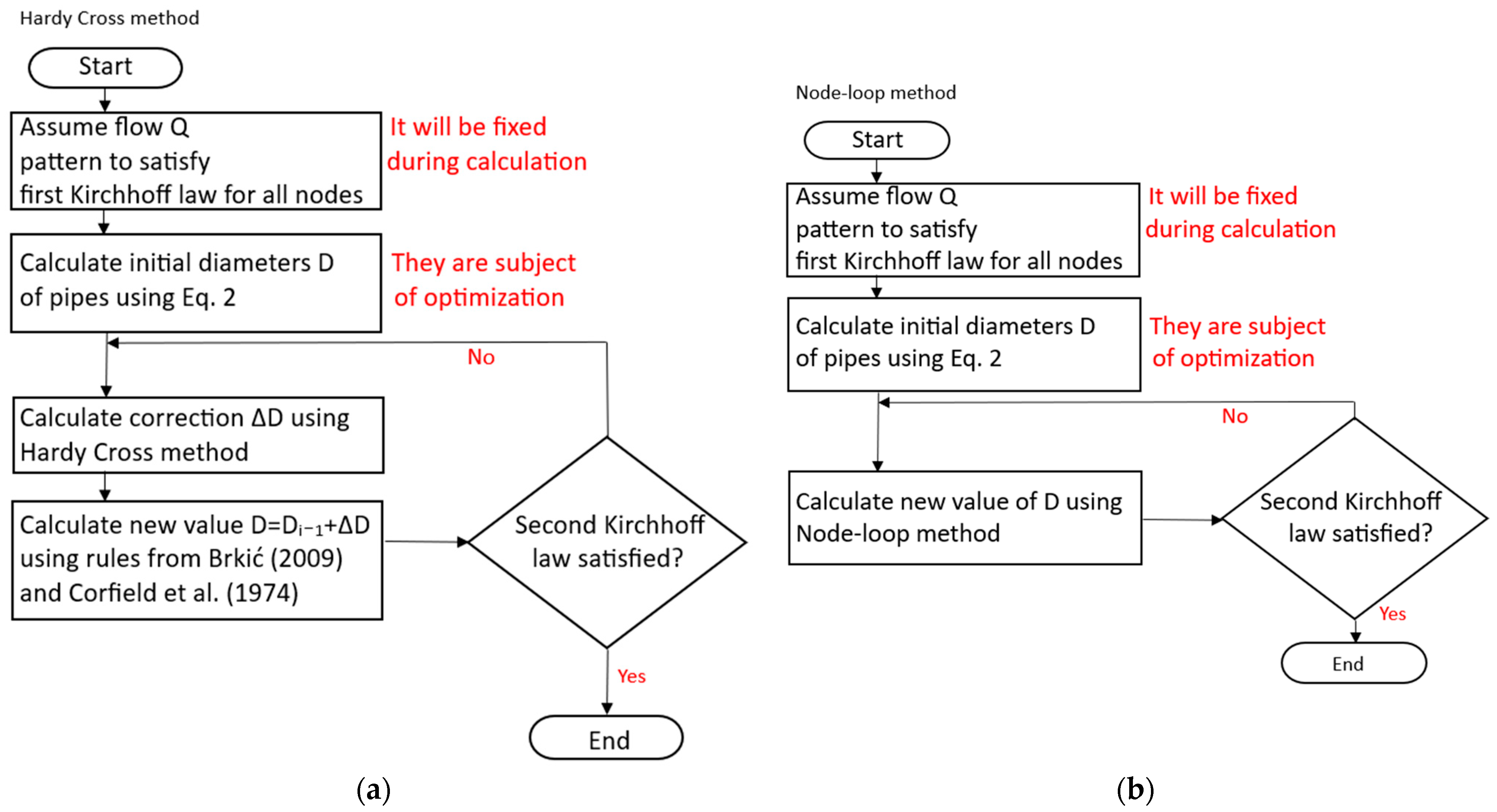
- Optimisation problem (subject of this article): In gas distribution network design and operation, it is essential to determine the optimal pipe diameters to minimise energy losses and ensure efficient gas flow. Pipe diameter calculations are often intertwined with flow and pressure calculations, requiring an iterative approach to find the best compromise between the pipe size and price. By adjusting parameters like the pipe diameter and pressure settings, network operators can aim for an ideal balance between the satisfaction of consumers and operational expenses. In the optimisation problem, the distribution of flow through the branches of a network of pipes (flow pattern) is known in advance and is not subject to changes during calculation (it is decided to keep the velocity of gas below certain prescribed technical limits, to allow the further expansion of the network or to satisfy a future increase in consumption and demand). Following the diagrams from Figure 1, this article provides two iterative methods for the optimisation of the pipe diameters for a fixed flow rate.
- Hardy Cross method with the correction of the diameter ΔD in each iteration: D = Di−1 + ΔD; see Figure 1a and Section 2.3.1 of this article.
- Node-loop method with the direct calculation of the diameter in each iteration: direct calculation of D; see Figure 1b and Section 2.3.2 of this article.
The difference between an approach with diameter corrections D = Di−1 + ΔD and the direct calculation of diameter D is given in Figure 1.
It should be noted that the solution of the optimisation problem is not unique and that infinite possible combinations of diameters can achieve mass continuity and the balance of energy through the network, satisfying both Kirchhoff’s first and second laws (on the contrary, a classical flow distribution problem where the diameters cannot be changed has a unique solution [36]). Although the Hardy Cross method and the node-loop method result typically in different pipe diameters, both can be used in the design phase and the final decision should be according to the preferences of the designer to fulfil certain goals and objectives (see Introduction).
2.1. Literature Overview
The main findings from the used literature that are useful for the presented optimisation are as follows:
- Detailed explanation of the correction of flow ΔQ in the Hardy Cross method [7] (with application to the correction of diameters ΔD during optimisation);
- Explanations of the first and second Kirchhoff laws for nodes and loops [12];
- Hydraulic models and equations for gas flow and its connection to the pressure drop [18];
- Classical versus optimisation approach applied to water distribution networks [22];
- A book with explanations of various methods for flow networks with loops applied to water distribution [25];
- Flow pattern in already existing pipe network with loops [36];
- Very illustrative but simple example of application of Hardy Cross and node-loop methods for water distribution [37];
- Approach involving virtual loop that connects two nodes with the same pressure in order to ensure a linear independent matrix needed for calculation (also application of the methods to ventilation systems of underground mines) [39];
- Safety [101].
2.2. Relation among Gas Flow, Pressure and Pipe Diameter
In the case of gas flow through plastic pipes, the relative roughness can usually be disregarded, making the flow regime hydraulically smooth [1,2]. Gas is a compressible fluid exposed to higher pressure in a typical city gas distribution network compared to atmospheric pressure, resulting in its decreased volume. As a result, the same mass of gas occupies a smaller volume than under normal (or standard) conditions, as in the case in this article, where Qst:Q ≈ 4. However, as it is already compressed, and due to the minimal pressure oscillations within the network, it can be treated as incompressible for the purpose of this calculation. The Renouard relation for gas flow in such conditions is given in Equation (1) [68,69,102]:
where
F is the pressure relation (Pa2);
p is the pressure (Pa);
is the relative density of natural gas (dimensionless); here, .64;
L is the pipe length (m);
Qst is the gas flow at standard conditions (m3/s), i.e., at standard pressure pst of 105 Pa and standard temperature of 15 °C (on the other hand, normal temperature for the same pressure is at 0 °C);
D is the inner pipe diameter (m);
’ denotes the first derivative; and
denotes the partial derivative.
The Renouard relation is derived for city gas, which mostly consists of carbon monoxide, predominantly produced from coal [85,86,87], now abandoned for gas distribution and replaced with natural gas. However, it is also extensively used for natural gas under relatively lower pressure (a few times higher than the atmospheric pressure) and for systems with plastic pipes, as is the case here. Hopefully, it can be used in systems with blended natural gas and hydrogen [60,61,62,63,64,65,66], as well as gasses produced from waste gasification [63,64].
The relation for the diameter is given in Equation (2):
where
D is the inner pipe diameter (m);
Q is the gas flow through the pipe in real conditions of pressure and temperature (m3/s); note that the Renouard relation, on the contrary, operates with Qst, gas flow at standard conditions;
pst is the standard pressure of 105 Pa;
u is the gas velocity (m/s); here, used for optimisation, u = 15 m/s;
p is the real pressure in pipes (Pa); here, p/pst ≈ 4;
π is the Ludolpf number ≈ 3.1415.
Pipe diameters as part of a gas network with loops are optimised in this article, which is a different problem [88,89,90] compared to determining the diameter of a single pipe (a solution to the problem of a single pipe in particular conditions is given in [91,92,93,103]). In any case, pipes are standardised and therefore they must be chosen from the prescribed list available for sale on the market [94].
2.3. Iterative Methods for Optimisation of Pipe Diameters
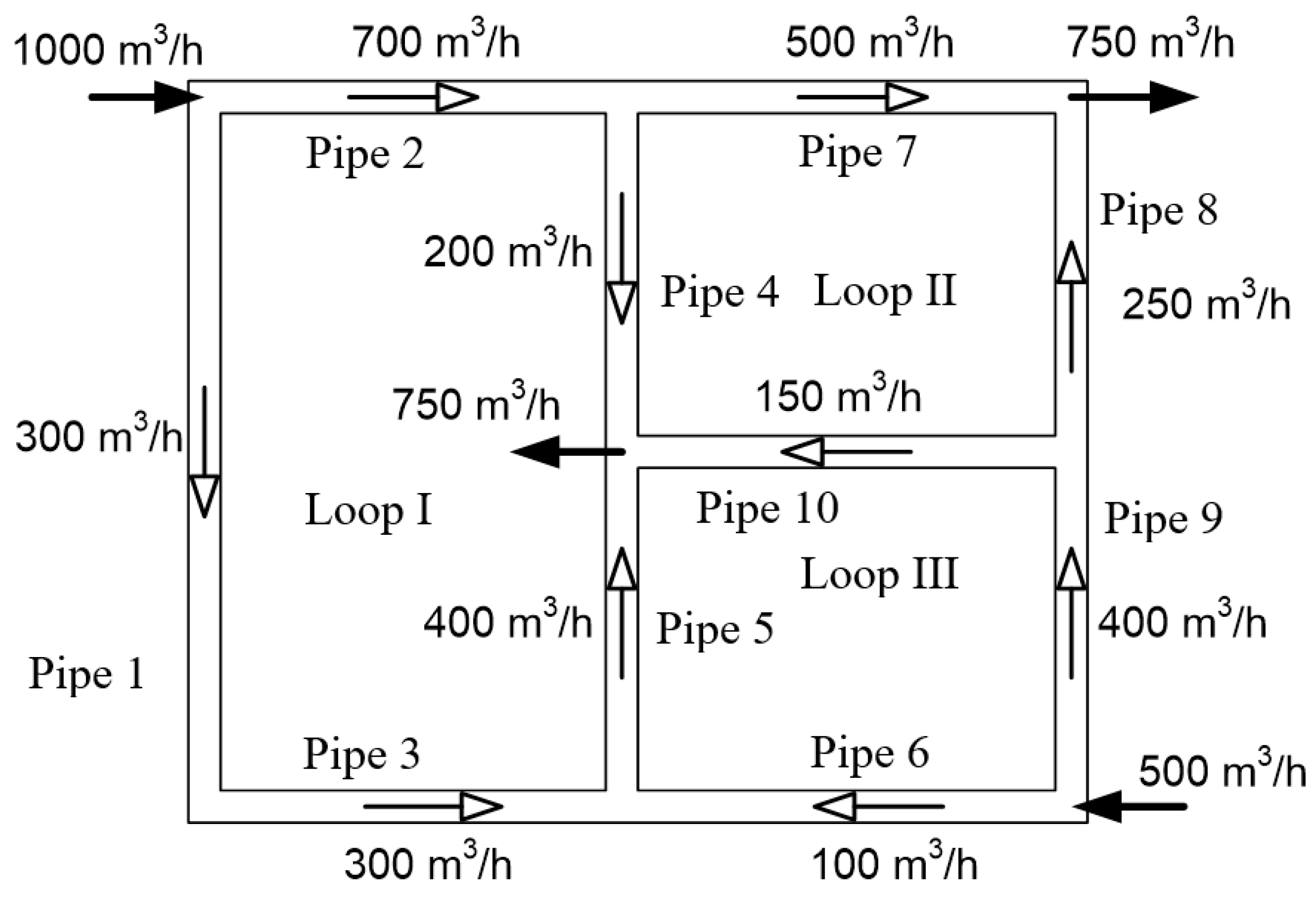
Two proposed iterative methods for the optimisation of pipe diameters based on the principles of the loop-oriented Hardy Cross method are explained in an illustrative network in Figure 2. The white arrows in Figure 2 represent the flow through the pipes, while the black arrows denote the consumption and supply of gas assigned to nodes (they also form virtual pipes for the purpose of the optimisation methods explained in this article).
The network consists of ten pipes and has eight interconnections of pipes (nodes) where these quantities are related to the Euler polyhedron formula from the topology [95,96] (used, e.g., in crystallography [97]). As given in Table 1, it has two inflow points of gas (the interconnections of pipes 1 and 2 and of pipes 6 and 9) and two outflow points of gas (the interconnections of pipes 7 and 8 and of pipes 4, 5 and 10).
The distribution of the flow through the pipes is established to satisfy consumers at peak demand and to satisfy flow continuity for each interconnection (node) in the network, following the requirements posed with Kirchhoff’s first law, as given in Table 2, where these values are fixed for the whole calculation using the presented iterative methods. The flow rates in each pipe, shown in Table 2, should be based on engineering judgement and prediction based on experience where the main consumers are located or will be located. The values of the flow rates through the pipes will not change through the shown iterative procedures for the optimisation of pipe diameters.
The goal is to adjust pipe diameter D in the network with loops to satisfy the energy balance by the second Kirchhoff law for every closed path of pipes in the network, i.e., to reach the algebraic sum of the pressure function F for each closed path to be approximately zero, , which is provided for the given illustrative network in Equation (3):
where , and are pressure functions (Pa2) with reference to the flow directions through the pipes in Loop I, Loop II and Loop III, respectively, in a counterclockwise direction. At the end of calculation, when the network is in balance, , and .
2.3.1. Improved Hardy Cross Method
The Hardy Cross method in its original form [3] can easily be used manually but its convergence is slow. In 1970, Epp and Fowler [38] accelerated the method, which is used as a basis for the iterative optimisation of the diameters in looped networks of pipes shown here. This improved version requires matrix calculation. The original vs. the improved version of the Hardy Cross method for the classical gas distribution problem was shown by Brkić in 2009 [5], while, in this article, the improved method is used for the optimisation of the pipe diameters in the gas distribution network from Figure 2.
In the original Hardy Cross method adjusted for diameter optimisation [61,66], the correction of diameter Δ for each pipe in the particular loop from Figure 2 is calculated using Equation (4):
Equation (4) can be expressed in matrix form as in Equation (5):
In Equations (4) and (5), F is calculated using Equation (3), i represents the count of iterations, and , and represent the first derivatives of the pressure function for the diameter as a variable, as given in Equation (6):
Finally, the improved (accelerated) method that converges faster is given in Equation (7):
In Equation (7), F′ is defined as , and .
The terms in the diagonal of the first matrix in Equation (7) are positive and all others are negative, while the matrix is symmetrical with respect to the main diagonal.
For each pipe in Loop I, correction should be multiplied by −1 and added algebraically to the diameter of each pipe, e.g., D1 + (−1)·, etc. Additionally, some pipes share two loops and they need to receive both corrections [5,37], from the adjacent loop without multiplication with −1, i.e., without a change in sign, e.g., for Loop I, D4 + (−1)·+, while, for Loop II, D4 + (−1)·+.
The values obtained for the first iteration using the accelerated method are given in Equation (8):
The final results using the accelerated method (Improved Hardy Cross Method) are listed in Section 3.
2.3.2. Node-Loop Method
The node-loop method has similar converging properties, i.e., it requires similar numbers of iterations to reach a balanced solution as the improved Hardy Cross. The main advantage of the node-loop method is that it directly provides a new value of the diameter D in each subsequent iteration, rather than a correction of flow ΔD as in the original and the improved Hardy Cross. For the classical gas distribution problem solved with the node-loop method, Brkić and Praks from 2019 can be consulted [6].
A new value of the diameter in each new iteration is calculated according to the node-loop method using Equation (9):
where [NL] and [V] are given in Equations (10) and (11), respectively, and where × means matrix multiplication.
In the node-Loop matrix for the illustrative network from Figure 2, the first seven rows are for nodes (interconnection of pipes) while the last three are for loops (closed paths of pipes). The network has eight nodes, while seven are arbitrarily kept for the calculation to preserve the linear independence (a slightly different approach with an additional pseudo-loop can be seen in [39]). Columns refer to pipes.
The same nodes as used for the first seven rows of [NL] are used in the first seven rows of the unique column of matrix [V] as given in Equation (11). For example, the node in the intersection of pipes 6 and 9 has an input of gas of 500 m3/h (+0.13889 m3/s) at standard conditions of pressure and temperature (Figure 2 and Table 1), and the diameter of the virtual pipe (black arrows in Figure 2) for this flow should be calculated using Equation (2) and multiplied by −1 (taken with opposite sign), while the virtual diameters will not be changed throughout the whole iterative calculation. The last three rows of [V] refer to loops and are calculated as given.
The final results using the Node-Loop Method are listed in Section 3.
3. Results and Discussion—Selection of Standardised Diameters
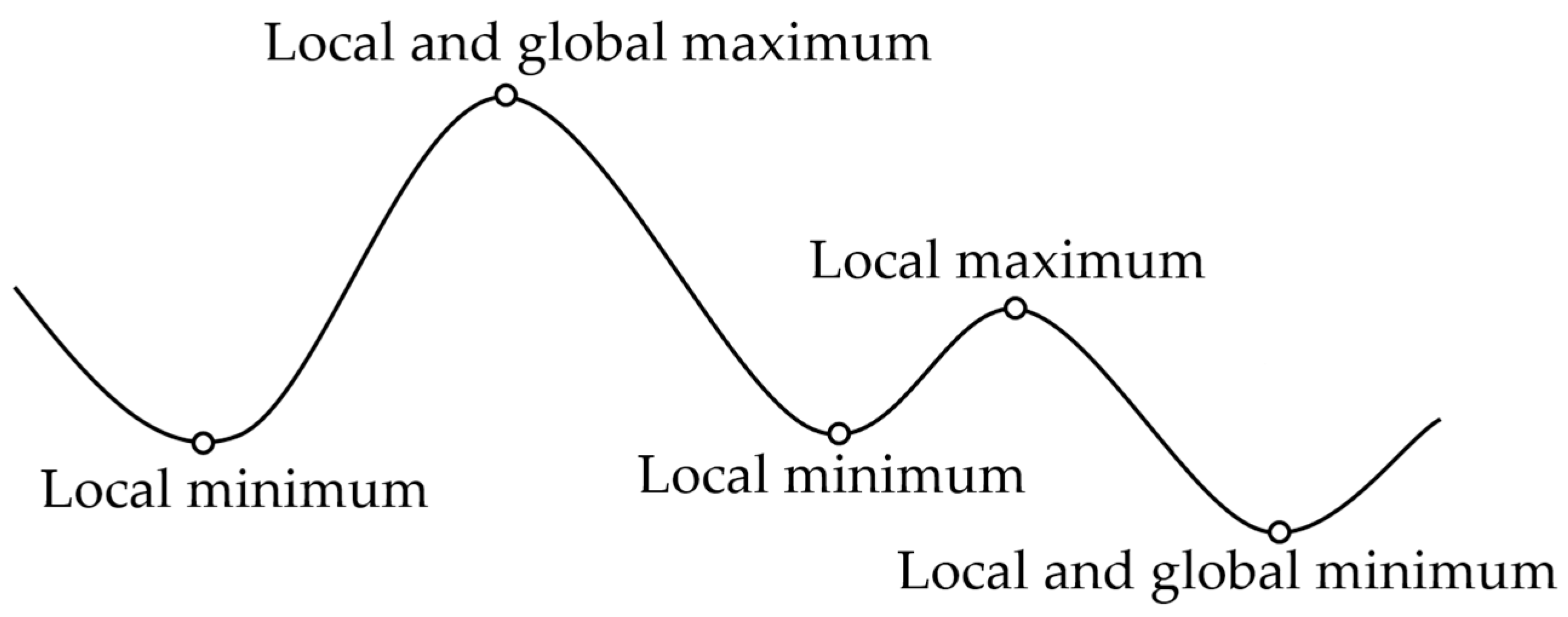
The results of the optimisation of the diameters in the illustrative network of pipes from Figure 2 are given in Table 3. The results are obtained after 10 iterations for both the improved Hardy Cross method and the node-loop method; they are also different, which is possible because the optimisation problem has an infinite number of solutions. The reason for the different final results, although the initial values are identical, is that some optimisation maximums or minimums are skipped in one method and taken by another (an infinite number of combinations can satisfy the second Kirchhoff law).
Based on the calculated diameters, using the velocity of the gas through the pipes, standard diameters should be selected from the appropriate catalogues [94] to reduce or to increase the velocity (larger diameter reduces velocity and vice versa).
The different values for the optimised diameters obtained using the two presented methods can be explained using the general illustrative example in Figure 3, where the two methods select different maximal and minimal values of the optimisation function.
4. Conclusions
The two presented methods typically give different final results, caused by overseeing the local extrema of the optimisation function due to the different steps during the calculation. A typical outcome will involve half of the pipes having a larger diameter and the other half having a smaller diameter, or with all pipes having similar and moderate values for the diameters. Between these two options, a designer should choose one based on the available stock of pipes or based on the future expansion of the network, places where larger consumers or many smaller consumers are located, etc. Whichever of the two options is chosen, the network will be balanced in terms of the velocity of gas during extreme conditions.
The appropriate steps would be as follows:
- Estimate consumption (maximal amount of gas consumed by households or industry);
- Assign the consumption to the nodes of the future network and choose locations for the nodes (it is fixed during calculation);
- Connect nodes with pipes, forming closed paths, i.e., loops (assign length of pipes, but not diameter);
- Redistribute the desired flow through the network considering the first Kirchhoff law for every node (it is fixed during calculation);
- Calculate the initial diameters using Equation (2) and optimise them using the methods shown;
- Select the diameters from the standardised values using the recommendations from Table 3;
Funding
From the Czech Republic: This work was supported by the ACROSS project. This project has received funding from the European High-Performance Computing Joint Undertaking (JU) under grant agreement No. 955648. The JU receives support from the European Union’s Horizon 2020 research and innovation programme and Italy, France, the Czech Republic, the United Kingdom, Greece, the Netherlands, Germany and Norway. This project has received funding from the Ministry of Education, Youth and Sports of the Czech Republic (ID: MC2104) and e-INFRA CZ (ID:90254). From Serbia: This work was supported by the Ministry of Science, Technological Development and Innovation of the Republic of Serbia through the institutional financing of the author (451-03-89647/2023-01/200102) from the 3rd of February 2023.
Data Availability Statement
All data that are necessary to repeat this research are available in the text.
Conflicts of Interest
The author declares no conflicts of interest.
References
- Manojlović, V.; Arsenović, M.; Pajović, V. Optimized design of a gas-distribution pipeline network. Appl. Energy 1994, 48, 217–224. [Google Scholar] [CrossRef]
- Brkić, D. A gas distribution network hydraulic problem from practice. Petr. Sci. Technol. 2011, 29, 366–377. [Google Scholar] [CrossRef]
- Cross, H. Analysis of Flow in Networks of Conduits or Conductors; University of Illinois at Urbana Champaign, College of Engineering Experiment Station: College Station, TX, USA, 1936; Available online: http://hdl.handle.net/2142/4433 (accessed on 3 October 2023).
- Brkić, D.; Praks, P. Short overview of early developments of the Hardy Cross type methods for computation of flow distribution in pipe networks. Appl. Sci. 2019, 9, 2019. [Google Scholar] [CrossRef]
- Brkić, D. An improvement of Hardy Cross method applied on looped spatial natural gas distribution networks. Appl. Energy 2009, 86, 1290–1300. [Google Scholar] [CrossRef]
- Brkić, D.; Praks, P. An efficient iterative method for looped pipe network hydraulics free of flow-corrections. Fluids 2019, 4, 73. [Google Scholar] [CrossRef]
- Corfield, G.; Hunt, B.E.; Ott, R.J.; Binder, G.P.; Vandaveer, F.E. Distribution design for increased demand. In Gas Engineers Handbook; Segeler, C.G., Ed.; Chapter 9; Industrial Press: New York, NY, USA, 1974; pp. 63–83. [Google Scholar]
- Cross, H. Analysis of continuous frames by distributing fixed-end moments. Trans. Am. Soc. Civ. Eng. 1932, 96, 1–10. [Google Scholar] [CrossRef]
- Volokh, K.Y. On foundations of the Hardy Cross method. Int. J. Solids Struct. 2002, 39, 4197–4200. [Google Scholar] [CrossRef]
- Baugh, J.; Liu, S. A general characterization of the Hardy Cross method as sequential and multiprocess algorithms. Structures 2016, 6, 170–181. [Google Scholar] [CrossRef]
- Reza, F. Some topological considerations in network theory. IRE Trans. Circuit Theory 1958, 5, 30–42. [Google Scholar] [CrossRef]
- Kirby, E.C.; Mallion, R.B.; Pollak, P.; Skrzyński, P.J. What Kirchhoff actually did concerning spanning trees in electrical networks and its relationship to modern graph-theoretical work. Croatica Chemica Acta 2016, 89, 403–417. [Google Scholar] [CrossRef]
- Ekhtiari, A.; Dassios, I.; Liu, M.; Syron, E. A novel approach to model a gas network. Appl. Sci. 2019, 9, 1047. [Google Scholar] [CrossRef]
- Farzaneh-Gord, M.; Rahbari, H.R. Unsteady natural gas flow within pipeline network, an analytical approach. J. Nat. Gas Sci. Eng. 2016, 28, 397–409. [Google Scholar] [CrossRef]
- Amani, H.; Kariminezhad, H.; Kazemzadeh, H. Development of natural gas flow rate in pipeline networks based on unsteady state Weymouth equation. J. Nat. Gas Sci. Eng. 2016, 33, 427–437. [Google Scholar] [CrossRef]
- Walters, G.; Swan, D.; Smith, D. Pipe system pressure probabilities with fluctuating demands. Civ. Eng. Syst. 1993, 10, 259–274. [Google Scholar] [CrossRef]
- Sircar, A.; Yadav, K. Optimization of city gas network: A case study from Gujarat, India. SN Appl. Sci. 2019, 1, 769. [Google Scholar] [CrossRef]
- Coelho, P.M.; Pinho, C. Considerations about equations for steady state flow in natural gas pipelines. J. Braz. Soc. Mech. Sci. Eng. 2007, 29, 262–273. [Google Scholar] [CrossRef]
- Niazkar, M.; Afzali, S.H. Analysis of water distribution networks using MATLAB and Excel spreadsheet: Q-based methods. Comput. Appl. Eng. Educ. 2017, 25, 277–289. [Google Scholar] [CrossRef]
- Niazkar, M.; Afzali, S.H. Analysis of water distribution networks using MATLAB and Excel spreadsheet: H-based methods. Comput. Appl. Eng. Educ. 2017, 25, 129–141. [Google Scholar] [CrossRef]
- Niazkar, M.; Eryılmaz Türkkan, G. Application of third-order schemes to improve the convergence of the Hardy Cross method in pipe network analysis. Adv. Math. Phys. 2021, 2021, 6692067. [Google Scholar] [CrossRef]
- Brkić, D. Spreadsheet-based pipe networks analysis for teaching and learning purpose. Spreadsheets Educ. 2016, 9, 4646. Available online: https://sie.scholasticahq.com/article/4646.pdf (accessed on 3 October 2023).
- Spiliotis, M.; Tsakiris, G. Water distribution system analysis: Newton-Raphson method revisited. J. Hydraul. Eng. 2011, 137, 852–855. [Google Scholar] [CrossRef]
- Simpson, A.; Elhay, S. Jacobian matrix for solving water distribution system equations with the Darcy-Weisbach head-loss model. J. Hydraul. Eng. 2011, 137, 696–700. [Google Scholar] [CrossRef]
- Boulos, P.F.; Lansey, K.E.; Karney, B.W. Comprehensive Water Distribution Systems Analysis Handbook for Engineers and Planners, 2nd ed.; MWH: Broomfield, CO, USA, 2006. [Google Scholar]
- Lopes, A.M.G. Implementation of the Hardy-Cross method for the solution of piping networks. Comput. Appl. Eng. Educ. 2004, 12, 117–125. [Google Scholar] [CrossRef]
- Huddleston, D.H.; Alarcon, V.J.; Chen, W. Water Distribution network analysis using Excel. J. Hydraul. Eng. 2004, 130, 1033–1035. [Google Scholar] [CrossRef]
- Wood, D.J.; Charles, C.O.A. Hydraulic network analysis using linear theory. J. Hydraul. Div. Am. Soc. Civ. Eng. 1972, 98, 1157–1170. [Google Scholar] [CrossRef]
- Wood, D.J.; Rayes, A.G. Reliability of algorithms for pipe network analysis. J. Hydraul. Div. Am. Soc. Civ. Eng. 1981, 107, 1145–1161. [Google Scholar] [CrossRef]
- Mah, R.S.H.; Lin, T.D. Comparison of Modified Newton’s methods. Comput. Chem. Eng. 1980, 4, 75–78. [Google Scholar] [CrossRef]
- Mah, R.S.H.; Shacham, M. Pipeline network design and synthesis. Adv. Chem. Eng. 1978, 10, 125–209. [Google Scholar] [CrossRef]
- Mah, R.S.H. Pipeline network calculations using sparse computation techniques. Chem. Eng. Sci. 1974, 29, 1629–1638. [Google Scholar] [CrossRef]
- Hamam, Y.M.; Brameller, A. Hybrid method for the solution of piping networks. Proc. Inst. Electr. Eng. 1971, 118, 1607–1612. [Google Scholar] [CrossRef]
- Shamir, U.; Howard, C.D.D. Water distribution systems analysis. J. Hydraul. Div. Am. Soc. Civ. Eng. 1968, 94, 219–234. [Google Scholar] [CrossRef]
- Ateş, S. Hydraulic modelling of closed pipes in loop equations of water distribution networks. Appl. Math. Model. 2016, 40, 966–983. [Google Scholar] [CrossRef]
- Gay, B.; Middleton, P. The solution of pipe network problems. Chem. Eng. Sci. 1971, 26, 109–123. [Google Scholar] [CrossRef]
- Brkić, D. Discussion of “Economics and statistical evaluations of using Microsoft Excel Solver in pipe network analysis” by Oke, I.A.; Ismail, A.; Lukman, S.; Ojo, S.O.; Adeosun, O.O.; Nwude, M.O. J. Pipeline Syst. Eng. Pract. 2018, 9, 7018002. [Google Scholar] [CrossRef]
- Epp, R.; Fowler, A.G. Efficient code for steady-state flows in networks. J. Hydraul. Div. Am. Soc. Civ. Eng. 1970, 96, 43–56. [Google Scholar] [CrossRef]
- Mathews, E.H.; Köhler, P.A.J. A numerical optimization procedure for complex pipe and duct network design. Int. J. Numer. Methods Heat Fluid Flow 1995, 5, 445–457. [Google Scholar] [CrossRef]
- Jha, K.; Mishra, M.K. Object-oriented integrated algorithms for efficient water pipe network by modified Hardy Cross technique. J. Comput. Des. Eng. 2020, 7, 56–64. [Google Scholar] [CrossRef]
- da Silva Teixeira, G.; Alonso, G.V.; Mendes, L.J. Evaluation of Nonlinear Iterative Methods on Pipe Network//Evaluación de Métodos Iterativos no Lineales en Redes de Tuberías. Ingeniería Mecánica 2021, 24, e656. Available online: https://ingenieriamecanica.cujae.edu.cu/index.php/revistaim/article/view/656 (accessed on 27 November 2023).
- Pons Poblet, J.M. The Hardy Cross method and its implementation in Spain. Revista Digital Lampsakos 2020, 1, 56–69. [Google Scholar] [CrossRef]
- Gokyay, O. An easy MS Excel software to use for water distribution system design: A real case distribution network design solution. J. Appl. Water Eng. Res. 2020, 8, 290–297. [Google Scholar] [CrossRef]
- Demir, S.; Karadeniz, A.; Yörüklü, H.C.; Demir, N.M. An MS Excel tool for parameter estimation by multivariate nonlinear regression in environmental engineering education. Sigma J. Eng. Nat. Sci. 2017, 35, 265–273. [Google Scholar] [CrossRef]
- Jaramillo, A.; Saldarriaga, J. Fractal analysis of the optimal hydraulic gradient surface in water distribution networks. J. Water Resour. Plan. Manag. 2023, 149, 4022074. [Google Scholar] [CrossRef]
- Martin-Candilejo, A.; Santillán, D.; Garrote, L. Pump Efficiency analysis for proper energy assessment in optimization of water supply systems. Water 2020, 12, 132. [Google Scholar] [CrossRef]
- Raoni, R.; Secchi, A.R.; Biscaia, E.C., Jr. Novel method for looped pipeline network resolution. Comput. Chem. Eng. 2017, 96, 169–182. [Google Scholar] [CrossRef]
- Sugishita, K.; Abdel-Mottaleb, N.; Zhang, Q.; Masuda, N. A growth model for water distribution networks with loops. Proc. R. Soc. A Math. Phys. Eng. Sci. 2021, 477, 20210528. [Google Scholar] [CrossRef]
- Zhong, D.; Wang, L.; Wang, J.; Jia, M. An efficient mine ventilation solution method based on minimum independent closed loops. Energies 2020, 13, 5862. [Google Scholar] [CrossRef]
- Dziurzyński, W.; Krach, A.; Pałka, T. Airflow sensitivity assessment based on underground mine ventilation systems modeling. Energies 2017, 10, 1451. [Google Scholar] [CrossRef]
- Pach, G.; Różański, Z.; Wrona, P.; Niewiadomski, A.; Zapletal, P.; Zubíček, V. Reversal ventilation as a method of fire hazard mitigation in the mines. Energies 2020, 13, 1755. [Google Scholar] [CrossRef]
- McPherson, M.J. Ventilation network analysis. Subsurf. Vent. Environ. Eng. 1993, 209–240. [Google Scholar] [CrossRef]
- Zhou, L.; Bahrami, D. A derivative method to calculate resistance sensitivity for mine ventilation networks. Min. Metall. Explor. 2022, 39, 1833–1839. [Google Scholar] [CrossRef]
- Jokić, A.; Zavargó, Z. Optimization of pipeline network for oil transport. Hung. J. Ind. Chem. 2001, 29, 113–117. [Google Scholar] [CrossRef]
- Kazemzadeh, H.; Amani, H.; Kariminezhad, H. Evaluation of pipeline networks to predict an increase in crude oil flow rate. Int. J. Press. Vessel. Pip. 2021, 191, 104374. [Google Scholar] [CrossRef]
- Shestakov, R.A. Research of distribution of oil flow in the pipeline with looping. J. Phys. Conf. Ser. 2020, 1679, 052035. [Google Scholar] [CrossRef]
- Talebi, B.; Mirzaei, P.A.; Bastani, A.; Haghighat, F. A review of district heating systems: Modeling and optimization. Front. Built Environ. 2016, 2, 22. [Google Scholar] [CrossRef]
- Guelpa, E. Impact of network modelling in the analysis of district heating systems. Energy 2020, 213, 118393. [Google Scholar] [CrossRef]
- Murat, J.; Smyk, A.; Laskowski, R.M. Selecting optimal pipeline diameters for a district heating network comprising branches and rings, using graph theory and cost minimization. J. Power Technol. 2018, 98, 30–44. Available online: https://papers.itc.pw.edu.pl/index.php/JPT/article/view/1287 (accessed on 11 October 2023).
- Eames, I.; Austin, M.; Wojcik, A. Injection of gaseous hydrogen into a natural gas pipeline. Int. J. Hydrog. Energy 2022, 47, 25745–25754. [Google Scholar] [CrossRef]
- Chandrasekar, A.; Syron, E. Evaluation of heat decarbonization strategies and their impact on the Irish gas network. Gases 2021, 1, 180–198. [Google Scholar] [CrossRef]
- Elaoud, S.; Hafsi, Z.; Hadj-Taieb, L. Numerical modelling of hydrogen-natural gas mixtures flows in looped networks. J. Pet. Sci. Eng. 2017, 159, 532–541. [Google Scholar] [CrossRef]
- Praks, P.; Lampart, M.; Praksová, R.; Brkić, D.; Kozubek, T.; Najser, J. Selection of appropriate symbolic regression models using statistical and dynamic system criteria: Example of waste gasification. Axioms 2022, 11, 463. [Google Scholar] [CrossRef]
- Praks, P.; Brkić, D.; Najser, J.; Najser, T.; Praksová, R.; Stajić, Z. Methods of Artificial Intelligence for Simulation of Gasification of Biomass and Communal Waste. In Proceedings of the 22nd International Carpathian Control Conference (ICCC), Velké Karlovice, Czech Republic, 31 May–1 June 2021. [Google Scholar] [CrossRef]
- Cheli, L.; Guzzo, G.; Adolfo, D.; Carcasci, C. Steady-state analysis of a natural gas distribution network with hydrogen injection to absorb excess renewable electricity. Int. J. Hydrog. Energy 2021, 46, 25562–25577. [Google Scholar] [CrossRef]
- Abbas, A.J.; Hassani, H.; Burby, M.; John, I.J. An investigation into the volumetric flow rate requirement of hydrogen transportation in existing natural gas pipelines and its safety implications. Gases 2021, 1, 156–179. [Google Scholar] [CrossRef]
- Vysocký, J.; Foltyn, L.; Brkić, D.; Praksová, R.; Praks, P. Steady-State Analysis of Electrical Networks in Pandapower Software: Computational Performances of Newton–Raphson, Newton–Raphson with Iwamoto Multiplier, and Gauss–Seidel Methods. Sustainability 2022, 14, 2002. [Google Scholar] [CrossRef]
- Renouard, M.P. Nouvelles règles à calcul pour la détermination des pertes de charge dans les conduites de gaz. J. Usines À Gaz 1952, 10, 337–339. (In French) [Google Scholar]
- Renouard, P. Méthode de calcul concernant l’écoulement du gaz en conduits. Travaux 1962, 329, 179. (In French) [Google Scholar]
- Piotrowski, R.; Ujazdowski, T. Designing control strategies of aeration system in biological WWTP. Energies 2020, 13, 3619. [Google Scholar] [CrossRef]
- Bagajewicz, M.; Valtinson, G. Computation of natural gas pipeline hydraulics. Ind. Eng. Chem. Res. 2014, 53, 10707–10720. [Google Scholar] [CrossRef]
- Ouyang, L.B.; Aziz, K. Steady-state gas flow in pipes. J. Pet. Sci. Eng. 1996, 14, 137–158. [Google Scholar] [CrossRef]
- Schroeder, D.W., Jr. A Tutorial on Pipe Flow Equations. In Proceedings of the PSIG Annual Meeting, Bonita Springs, FL, USA, 11–14 May 2010; Paper Number: PSIG-1008a. Available online: https://onepetro.org/PSIGAM/proceedings-abstract/PSIG10/All-PSIG10/2431 (accessed on 3 October 2023).
- Colebrook, C.F. Turbulent flow in pipes, with particular reference to the transition region between the smooth and rough pipe laws. J. Inst. Civ. Eng. 1939, 11, 133–156. [Google Scholar] [CrossRef]
- Brkić, D.; Stajić, Z. Excel VBA-based user defined functions for highly precise Colebrook’s pipe flow friction approximations: A comparative overview. Facta Univ. Ser. Mech. Eng. 2021, 19, 253–269. [Google Scholar] [CrossRef]
- Praks, P.; Brkić, D. Review of new flow friction equations: Constructing Colebrook’s explicit correlations accurately. Rev. Int. Metodos Numer. Calc. Diseño Ing. 2020, 36, 41. [Google Scholar] [CrossRef]
- Carvajal, J.; Zambrano, W.; Gómez, N.; Saldarriaga, J. Turbulent flow in PVC pipes in water distribution systems. Urban Water J. 2020, 17, 503–511. [Google Scholar] [CrossRef]
- Aynsley, R.M. A Resistance approach to analysis of natural ventilation airflow networks. J. Wind Eng. Ind. Aerodyn. 1997, 67–68, 711–719. [Google Scholar] [CrossRef]
- Anonymous. Pipeline-network analyzer. J. Frankl. Inst. 1952, 254, 195. [Google Scholar] [CrossRef]
- Taherinejad, M.; Hosseinalipour, S.M.; Madoliat, R. Dynamic simulation of gas pipeline networks with electrical analogy. J. Braz. Soc. Mech. Sci. Eng. 2017, 39, 4431–4441. [Google Scholar] [CrossRef]
- Toktoshov, G.Y. The routes choosing methodology for laying networks in three-dimensional space. In Proceedings of the 17th International Asian School-Seminar “Optimization Problems of Complex Systems (OPCS)”, Novosibirsk, Russian, 13–17 September 2021; pp. 139–143. [Google Scholar] [CrossRef]
- Zhao, Q.; Wu, W.; Simpson, A.R.; Willis, A. Simpler is better—Calibration of pipe roughness in water distribution systems. Water 2022, 14, 3276. [Google Scholar] [CrossRef]
- Chaubey, S.K.; Gupta, K.; Madić, M. An investigation on mean roughness depth and material erosion speed during manufacturing of stainless-steel miniature ratchet gears by wire-EDM. Facta Univ. Ser. Mech. Eng. 2023, 21, 239–258. [Google Scholar] [CrossRef]
- Chaubey, S.K.; Gupta, K. A review on Wire-EDM of bio titanium. Rep. Mech. Eng. 2023, 4, 141–152. [Google Scholar] [CrossRef]
- Odell, W.W. Facts Relating to the Production and Substitution of Manufactured Gas for Natural Gas (No. 301). Department of Commerce, Bureau of Mines. 1929. Available online: https://books.google.com/books?hl=en&lr=&id=st4RRgrGA3sC&oi=fnd&pg=PA1&ots=A0gdw9fRsE&sig=0jy_T3hokBlDwzEA9BtdO_ye5AY (accessed on 1 December 2023).
- Anonymous. Substitution of manufactured gas for natural gas. J. Frankl. Inst. 1930, 209, 121–125. [Google Scholar] [CrossRef]
- Rimos, S.; Hoadley, A.F.; Brennan, D.J. Determining the economic consequences of natural gas substitution. Energy Convers. Manag. 2014, 85, 709–717. [Google Scholar] [CrossRef]
- Featherstone, R.E.; El-Jumaily, K.K. Optimal diameter selection for pipe networks. J. Hydraul. Eng. 1983, 109, 221–234. [Google Scholar] [CrossRef]
- Arumugam, A.; Subramani, S.; Kibrom, H.; Gebreamlak, M.; Mengstu, M.; Teame, M. Comparison and validation of models for the design of optimal economic pipe diameters: A case study in the Anseba region, Eritrea. TecnoLógicas 2021, 24, e1992. [Google Scholar] [CrossRef]
- ElZahar, M.M.H.; Amin, M.M.M. Optimization of water pipe network and formulation of pumping rate. KSCE J. Civ. Eng. 2023, 27, 2882–2890. [Google Scholar] [CrossRef]
- Brkić, D.; Praks, P.; Praksová, R.; Kozubek, T. Symbolic regression approaches for the direct calculation of pipe diameter. Axioms 2023, 12, 850. [Google Scholar] [CrossRef]
- Lamri, A.A.; Easa, S.M. Explicit solution for pipe diameter problem using Lambert W-function. J. Irrig. Drain. Eng. 2022, 148, 04022030. [Google Scholar] [CrossRef]
- Brkić, D.; Stajić, Z.; Živković, M. Sizing pipes without iterative calculus: Solutions for head loss, flow discharge and diameter. In Proceedings of the 24th International Carpathian Control Conference, Szilvásvárad, Hungary, 12–14 June 2023. [Google Scholar] [CrossRef]
- ISO 6708:1995; Pipework Components—Definition and Selection of DN (Nominal Size). International Organization for Standardization,: Geneva, Switzerland. Available online: https://www.iso.org/standard/21274.html (accessed on 3 October 2023).
- Debnath, L. A brief historical introduction to Euler’s formula for polyhedra, topology, graph theory and networks. Int. J. Math. Educ. Sci. Technol. 2010, 41, 769–785. [Google Scholar] [CrossRef]
- Hu, G.; Qiu, W.Y.; Ceulemans, A. A new Euler’s formula for DNA polyhedra. PLoS ONE 2011, 6, e26308. [Google Scholar] [CrossRef]
- Pîrvan-Moldovan, A.; Diudea, M.V. Euler characteristic of polyhedral graphs. Croat. Chem. Acta 2016, 89, 471–479. [Google Scholar] [CrossRef]
- Alrumaih, T.N.; Alenazi, M.J. GENIND: An industrial network topology generator. Alex. Eng. J. 2023, 79, 56–71. [Google Scholar] [CrossRef]
- Filo, G. Artificial intelligence methods in hydraulic system design. Energies 2023, 16, 3320. [Google Scholar] [CrossRef]
- Tawfik, A.M. Hydraulic solutions of pipeline systems using artificial neural networks. Ain Shams Eng. J. 2023, 14, 101896. [Google Scholar] [CrossRef]
- Brkić, D.; Praks, P. Probability analysis and prevention of offshore oil and gas accidents: Fire as a cause and a consequence. Fire 2021, 4, 71. [Google Scholar] [CrossRef]
- Règle a Calcul Pertes de Charge Dans les Canalisations de gaz a Basse Pression (in French). Available online: https://photocalcul.com/Calcul/Regles/Notices-regles/notice_GraphoplexGDF_908445.pdf (accessed on 14 December 2023).
- Brkić, D.; Praks, P. Discussion of “Explicit solution for pipe diameter problem using Lambert W-function” by Lamri, A.A.; Easa, S.M. J. Irrig. Drain. Eng. 2023, 149, 07023016. [Google Scholar] [CrossRef]
Figure 1.
Differences between approaches of the two proposed loop-oriented methods for optimisation: (a) diameter correction D = Di−1 + ΔD, Hardy Cross method—Brkić (2009) [5] and Corfield et al. [7]; (b) direct calculation of D, node-loop method.

Figure 2.
Illustrative network of pipes with loops (black arrows represent inputs and outputs of the network, while white arrows are flows through pipes).
Figure 2.
Illustrative network of pipes with loops (black arrows represent inputs and outputs of the network, while white arrows are flows through pipes).

Figure 3.
Possible extrema of the optimisation function—general illustrative example.


Table 1.
Constant inflow and outflow of gas at interconnections of pipes.
| Nodes between/among Pipes | Inflow/Outflow 1 | Flow Qst | |
|---|---|---|---|
| m3/h | m3/s | ||
| 1 and 2 | Inflow | +1000 | +0.27778 |
| 6 and 9 | Inflow | +500 | +0.13889 |
| 4, 5 and 10 | Outflow | −750 | −0.20833 |
| 7 and 8 | Outflow | −750 | −0.20833 |
| Σ | 0 | 0 | |
1 plus sign denotes input of gas in the network, while minus sign denotes output.
Table 2.
Fixed flow of gas per pipe and initial pipe diameters.
| Pipe | Length L | Fixed flow Qst | 1 Initial Diameter D | |
|---|---|---|---|---|
| m | m3/h | m3/s | m | |
| 1 | 200 | 300 | 0.083333333 | 0.042052209 |
| 2 | 100 | 700 | 0.194444444 | 0.064235810 |
| 3 | 100 | 300 | 0.083333333 | 0.042052209 |
| 4 | 100 | 200 | 0.055555556 | 0.034335485 |
| 5 | 100 | 400 | 0.111111111 | 0.048557708 |
| 6 | 100 | 100 | 0.027777778 | 0.024278854 |
| 7 | 100 | 500 | 0.138888889 | 0.054289168 |
| 8 | 100 | 250 | 0.069444444 | 0.038388239 |
| 9 | 100 | 400 | 0.111111111 | 0.048557708 |
| 10 | 100 | 150 | 0.041666667 | 0.029735402 |
1 Using Equation (2).
Table 3.
Recapitulation of diameters with velocities.
| Initial | Improved Hardy Cross | Node Loop | ||||||
|---|---|---|---|---|---|---|---|---|
| Final | Standard Diameter Dn | Final | Standard Diameter Dn | |||||
| Pipe | 1 Diameter D | Velocity u | Diameter D | 2 Velocity u | Diameter D | 2 Velocity u | ||
| m | m/s | M | m/s | mm | m | m/s | mm | |
| 1 | 0.042052209 | 15 | 0.045862467 | 12.61 | 40 | 0.045306252 | 12.92 | 40 |
| 2 | 0.06423581 | 15 | 0.060425552 | 16.95 | 65 | 0.108246703 | 5.28 | 90 or 100 |
| 3 | 0.042052209 | 15 | 0.045862467 | 12.61 | 40 | 0.049136481 | 10.99 | 40 |
| 4 | 0.034335485 | 15 | 0.032068353 | 17.20 | 40 | 0.03146551 | 17.86 | 40 |
| 5 | 0.048557708 | 15 | 0.052026572 | 13.07 | 50 | 0.073402904 | 6.56 | 50 or 65 |
| 6 | 0.024278854 | 15 | 0.023937460 | 15.43 | 25 | 0.024266423 | 15.02 | 32 |
| 7 | 0.054289168 | 15 | 0.052746042 | 15.89 | 65 | 0.076781193 | 7.50 | 50 or 65 |
| 8 | 0.038388239 | 15 | 0.039931365 | 13.86 | 32 | 0.056199567 | 7.00 | 32 or 40 |
| 9 | 0.048557708 | 15 | 0.048899102 | 14.79 | 40 | 0.084311913 | 4.98 | 90 or 100 |
| 10 | 0.029735402 | 15 | 0.028533670 | 16.29 | 32 | 0.028112346 | 16.78 | 32 |
1 Repeated from Table 1. 2 If u > 15, a larger Dn should be selected, and if u < 15 m/s, a smaller Dn should be selected.
Disclaimer/Publisher’s Note: The statements, opinions and data contained in all publications are solely those of the individual author(s) and contributor(s) and not of MDPI and/or the editor(s). MDPI and/or the editor(s) disclaim responsibility for any injury to people or property resulting from any ideas, methods, instructions or products referred to in the content. |
© 2024 by the author. Licensee MDPI, Basel, Switzerland. This article is an open access article distributed under the terms and conditions of the Creative Commons Attribution (CC BY) license (https://creativecommons.org/licenses/by/4.0/).
Share and Cite
MDPI and ACS Style
Brkić, D. Two Iterative Methods for Sizing Pipe Diameters in Gas Distribution Networks with Loops. Computation 2024, 12, 25. https://doi.org/10.3390/computation12020025
AMA Style
Brkić D. Two Iterative Methods for Sizing Pipe Diameters in Gas Distribution Networks with Loops. Computation. 2024; 12(2):25. https://doi.org/10.3390/computation12020025
Chicago/Turabian StyleBrkić, Dejan. 2024. "Two Iterative Methods for Sizing Pipe Diameters in Gas Distribution Networks with Loops" Computation 12, no. 2: 25. https://doi.org/10.3390/computation12020025
Note that from the first issue of 2016, this journal uses article numbers instead of page numbers. See further details here.