Article

Data Augmentation for Regression Machine Learning Problems in High Dimensions

1
PIMM, Arts et Métiers Institute of Technology, 151 Boulevard de l’Hopital, 75013 Paris, France
2
UPR EBINNOV, Ecole de Biologie Industrielle, 49 Avenue des Genottes, 95895 Cergy, France
3
ESI Group, Parc Icade, Immeuble le Seville, 3bis, Saarinen, CEDEX, 94528 Rungis, France
4
CNRS@CREATE Ltd., 1 Create Way, 08-01 CREATE Tower, Singapore 138602, Singapore
*
Author to whom correspondence should be addressed.
Computation 2024, 12(2), 24; https://doi.org/10.3390/computation12020024
Submission received: 24 November 2023 / Revised: 5 January 2024 / Accepted: 23 January 2024 / Published: 1 February 2024

Abstract

:
Machine learning approaches are currently used to understand or model complex physical systems. In general, a substantial number of samples must be collected to create a model with reliable results. However, collecting numerous data is often relatively time-consuming or expensive. Moreover, the problems of industrial interest tend to be more and more complex, and depend on a high number of parameters. High-dimensional problems intrinsically involve the need for large amounts of data through the curse of dimensionality. That is why new approaches based on smart sampling techniques have been investigated to minimize the number of samples to be given to train the model, such as active learning methods. Here, we propose a technique based on a combination of the Fisher information matrix and sparse proper generalized decomposition that enables the definition of a new active learning informativeness criterion in high dimensions. We provide examples proving the performances of this technique on a theoretical 5D polynomial function and on an industrial crash simulation application. The results prove that the proposed strategy outperforms the usual ones.

1. Introduction

In the context of multi-parametric problems where one wants to estimate an output value, Y, that depends on multiple input variables, X = ( x 1 , . . . , x n ) , it is usual to resort to machine learning [1]. To do so, an algorithm is trained on a few examples grouped as a training database ( X t r a i n i n g , Y t r a i n i n g ) to be able then to make predictions for unknown cases, X t e s t . The design of the training database is a main issue because it partly determines the performances of the algorithm (i.e., the further predictions). However, the generation of training samples if often costly. For instance, it can be really time-consuming to run simulations or to realize experiments. It can also be relatively expensive because of the cost of access to servers or machines.
Moreover, as the problems considered nowadays become more and more complex, and depend on many input parameters, the models need many samples to be trained. This issue is known as the “curse of dimensionality” [2]. Indeed, the volume of the space increases so fast that the data become sparse and the number of necessary points needed to approximate the space increases too. Therefore, for these reasons, the samples employed by the algorithm need to be chosen efficiently.
Usually, training databases are constructed thanks to the methodology of Design of Experiments [3]. Therefore, another approach has been developed over the past few years with the emergence of active learning [4]. This technique proceeds by iteration with the assumption that adding at each step the sample that improves the model the most will increase the performances quickly. Different ways to evaluate informativeness of a sample regarding a specific model have been investigated. Various corresponding information criteria have also been defined for classification and regression. Nevertheless, many of them have failed when it comes to operating in high-dimensional settings.
Thus, we aim here to develop an efficient, iterative and automatic method to design a training set for high-dimensional regression problems. To address this issue, a new information criterion from a combination of the information given by the Fisher matrix [5] with sparse proper generalized decomposition (s-PGD) [6] has been defined. The proposed methodology is described in Section 2. It will be then tested on two different applications, a polynomial function and a crash simulation problem. The results obtained are presented in Section 3. Finally, the paper is completed with some concluding remarks in Section 4.

2. Methodology

To tackle the issue of high-dimensional regression problems, a new method for designing training databases has been defined following the steps of an active learning methodology. This method is based on the combination of the properties from the Fisher information matrix and a model order reduction method through the use of s-PGD.

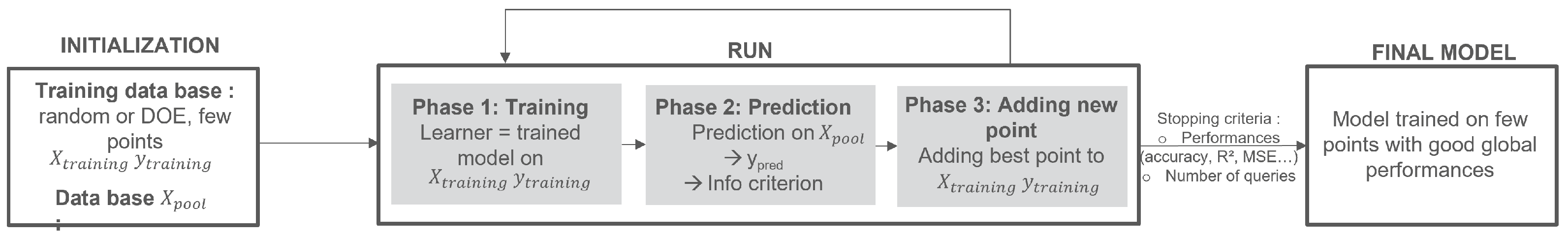
2.1. Active Learning

Firstly, various ways to design training databases for machine learning problems exist. One of the most classic ways to build these training databases is to resort to Design of Experiments (DOE). Indeed, DOE enables better organization of the tests performed in scientific research or industrial studies. Its objective is to extract the maximum information with a minimum number of experiments, and there are different ways in the literature to construct these plans such as full design [7], full factorial design [8], Plackett–Burman [9], Latin hypercube sampling (LHS), [10,11], etc.
However, their major disadvantage is that their conception only depends on the input space and does not take into consideration the output. Moreover, the number of data needed depends on the number of dimensions and levels chosen. Thus, the number often increases drastically with the number of dimensions, suffering from the “curse of dimensionality”. That is why other iterative and automatic methods have subsequently been developed, like active learning methods.
The main idea of active learning is summed up in Figure 1. A machine learning algorithm will be able to achieve better performances with few training samples if it can choose the data from which it will learn. Therefore, the algorithms ask at each step for the real output value associated with a sample “query” that an external entity named “oracle” must then provide. It stops when the objective had been reached according to a stopping criterion.
As a result, active learning is particularly suitable in many current machine learning problems, where data can be time-consuming or expensive to obtain.

2.1.1. Scenarios

In active learning, there are different scenarios in which the queries can be made. Indeed, there are different ways to select or take a sample in order to add it to the training database of the trained model. That is why a quick overview of the query strategies proposed in the literature will be presented here.
The three main methods described in the literature and detailed after are: (i) membership query synthesis [12,13,14], (ii) stream-based selective sampling [15], and (iii) pool-based sampling [16].
(i)
Membership query synthesis [12]: here, the model can ask for any sample in the input space, and it can also ask for queries generated de novo rather than for those sampled from an underlying natural distribution. This method has been particularly effective for problems confined to a finite domain [13]. Initially developed for classification models, it can also be extended to regression models [14]. However, this method may leave too much freedom to the algorithm, which can be led to request samples without any physical meaning.
(ii)
Stream-based selective sampling [15]: here, the initial assumption is that it is not expensive to add a sample. Therefore, the model decides for each possible sample whether to add it as training data. This approach is also sometimes called stream-based or sequential active learning because all the samples are considered one by one and the model chooses for each one whether to keep it or not.
(iii)
Pool-based sampling [16]: here, a small set, L, of labeled data and a large set, denoted U, of unlabeled available data are considered. The query is then made according to the information criterion, which evaluates the relevance of a sample from the basis U in comparison with the others. The best sample according to this criterion is then chosen and added to the training set. The difference with the previous scenario is that the decision regarding a sample is taken individually. In pool-based sampling, the other samples still available are taken into account. This last method is the most used in real applications.
Next, to assess the relevance of a sample and to be able to apply these scenarios, it is necessary to quantify the information carried by a sample.

2.1.2. Query Strategies

The quantification of the information carried by a sample can also be diverse, and has led to the definition of various query strategies in the literature. The notation x A * refers to the most informative sample (i.e., the best or most relevant sample) for each of given method A. The input values are noted x, the outputs, y i , range over all possible labeling, i, and the model estimation, θ .
  • Uncertainty Sampling:
    Uncertainty sampling [16,17,18,19] considers that the most informative sample is the one the model is most uncertain to predict correctly. With the entropy definition from [19], this uncertainty can be written:
    x U S * = arg max x i P θ ( y i x ) l o g P θ ( y i x ) .
  • Query by Committee:
    A committee of models trained on different hypothesis on the base L is defined as C = θ ( 1 ) , . . . , θ ( C ) . Then, a vote is carried out and the sample that generates the most disagreement is selected and added [20]. There are different ways to measure the level of disagreement and make the final vote. The two most used are the vote entropy, described in [21], and the Kullback–Leibler (KL) divergence in [22].
  • Expected model change:
    For a given model and a given sample, the impact of the sample if added to the training database, L, is estimated through a gradient calculation. The sample that induces the biggest change is here the most relevant and is added to the training set [23,24]:
    x E M C * = arg max x i P θ ( y i x ) l θ ( x , y i ) ,
    where l θ ( x , y i ) is the gradient of the objective function, l, respectively, to the parameters, θ , applied to the tuple x , y i .
  • Variance reduction:
    The most informative sample that will be added to the training set is the one minimizing the output variance (i.e., minimizing the generalization error) [25]:
    x V R * = arg min x < σ y ^ 2 > + x ,
    where < σ y ^ 2 > + x is the estimated mean output variance across the input distribution after the model has been re-trained on the query, x, and its corresponding label.
Thanks to theses various definitions of scenarios and queries strategies, many methods of active sampling design can be set up.
Moreover, recent methods in active learning focus on addressing challenges such as sample diversity, model uncertainty, or computational efficiency. Techniques like query-by-committee and Bayesian methods have gained prominence. Advancements in deep learning have led to the development of active learning strategies tailored for neural networks [26] to tackle various applications [27,28]. Recent research has also explored innovative approaches, such as meta-learning for active learning [29,30,31] or incorporating human feedback into the loop [32].
In addition, new techniques based on D-optimality, like coordinate-exchange [33,34] or minmax criterion, [35] have been developed, or alternatives to LHS, like through augmenting supersaturated designs [36] or space-filling designs [37].
However, most of them do not work effectively for high-dimensional regression and few data. Indeed, in active learning methods, many criteria are defined with an euclidean distance x i x j between x i and x j points of the input space. In high dimensions, the distance between two points is high for any points. Therefore, the criterion has similar value for each point and cannot be used.

2.2. s-PGD Equations

On one hand, to deal with high-dimensional problems, a common solution is to resort to model order reduction (MOR) methods [38]. These methods allow the reduction of the computational complexity of mathematical models in numerical simulations. Indeed, even if using a reduced basis generates some loss of generality, it often allows impressive computing time savings. Moreover, if the problem solution is in the reduced basis, the calculated solution with MOR remains quite precise.
Different techniques exist. But, as the aim here is to focus on regression in high dimensions, PGD is very suitable since it overcomes the limitations of classical approaches. In particular, PGD avoids the curse of dimensionality, as solving decoupled problems is computationally much less expensive than solving multidimensional problems. Therefore, PGD enables the formulation of parametric problems into a multidimensional framework by setting the parameters of the problem as extra coordinates [39]. Then, a sparsely sampled counterpart, called sparse PGD (s-PGD), was proposed in [6] So, s-PGD is adapted for regression in high dimensions while using few data. It is the algorithm that will be used in this paper and summarized in what follows.
If we consider a function, f, in n dimensions:
f ( x 1 , . . . , x n ) : Ω R n R ,
where x 1 . . . x n are the input variables, and s-PGD can be expressed as the following decomposition:
f ( x 1 , . . . , x n ) f ˜ M ( x 1 , . . . , x n ) = m = 1 M k = 1 n X m k ( x k ) .
Then, X can be decomposed as:
X m k ( x k ) = j = 1 M N j , m k a j , m k = ( N m k ) T a m k ,
where M stands for the number of terms in the decomposition, N j , m k are the set of basis functions for the corresponding k t h dimension and m t h mode, and a j , m k are the coefficients for the corresponding k t h dimension and the m t h mode also.
These approximated functions, f ˜ M , are calculated step by step thanks to a greedy algorithm, and the new M t h order term is found using a non-linear solver (Picard or Newton, for instance):
f ˜ M = m = 1 M 1 k = 1 n X m k ( x k ) + k = 1 n X M k ( x k ) .
In a machine learning framework, this approximation allows us to make an estimation of the output values related to unknown data. Moreover, achieving this is particularly difficult when confronted with a high-dimensional problem, where the data are sparse and/or scarce. Indeed, the regression problem described here only guarantees that the minimization is satisfied by the training. Thus, if the sampling points in the training set are not numerous enough, high oscillations may appear out of these measured points because the risk of over-fitting has increased. This affects the predictions of the generated model.
To deal with this issue, a modal adaptivity strategy (MAS) can be set up. The idea of MAS is to minimize the oscillations outside the training set by starting the PGD algorithm with only low degree modes. When the residual values then decrease slowly enough or reach a fixed value, higher order approximation functions are added. This method has proven to be an efficient way to improve s-PGD performances in many cases [40,41,42,43]. However, some limitations remain. For instance, it has been noted that the desired accuracy is not achieved before reaching over-fitting or the algorithm can stop too early when using MAS in some cases. In addition, in problems where just a few terms of the interpolation basis are present, the method fails in identifying the true model and leads to bad predictions.
To solve these difficulties, other versions of PGD have been developed, such as the rs-PGD and the s2-PGD, as detailed in [39].

2.3. Fisher Matrix

On the other hand, to develop an active learning methodology, it is necessary to define an informativeness criterion. Yet, one way to quantify the information quarried in a series of observations is to use Fisher information [5,44], or, for n parameters, the corresponding Fisher information matrix.
The likelihood, f ( X , μ ) , is considered a function of X with respect to parameter μ . In statistics, the Fisher information is a way of measuring the information carried by an observable random variable about an unknown parameter, μ , of a distribution that models X.
Moreover, the main issue in defining a DOE is the ease of identifying parameters by maximizing the likelihood. Indeed, where f is sharply peaked with respect to changes in μ , the data provide much information about the parameter μ . Then, it is easy to indicate the “correct” value of μ from the data. On the contrary, if f is flat, many samples are needed to determine the actual parameter values with adequate accuracy. Therefore, the variance with respect to μ could be a valuable indicator to optimize the design.
To do so, the partial derivative with respect to μ of the log-likelihood, formally called score, s, can be written as:
s ( μ ) = log f ( X , μ ) μ .
Then, the variance of the score is by definition the Fisher information, I ,
I ( μ ) = V ( s ( μ ) ) = E ( s ( μ ) 2 ) ( E ( s ( μ ) ) ) 2 .
Under certain regularity conditions, the first moment of the score vanishes,
E ( s ( μ ) ) = E log f ( X , μ ) μ = f ( x , μ ) μ f ( x , μ ) f ( x , μ ) d x = μ f ( x , μ ) d x = μ 1 = 0 .
It gives
I ( μ ) = E log f ( X , μ ) μ 2 .
Which, taking into account
2 log f ( X , μ ) μ 2 = 2 f ( X , μ ) μ 2 f ( X , μ ) log f ( X , μ ) μ 2
and
E 2 f ( X , μ ) μ 2 f ( X , μ ) = 2 μ 2 f ( x , μ ) d x = 0
yields
I ( μ ) = E 2 μ 2 log f ( X , μ ) .
When considering many parameters, μ = ( μ 1 , μ 2 . . . , ) , the result is the so-called Fisher information matrix, whose components read,
I i , j ( μ ) = E μ i log f ( X , μ ) μ j log f ( X , μ ) ,
i.e.,
I ( μ ) = E log f ( X , μ ) log f ( X , μ ) T .

2.4. Computation of a New Information Criterion

The previous definition of Fisher information (16) can be applied to any model of X. Then, it can be applied to s-PGD (5).
For the ease of the exposition and without loss of generality, let us begin by assuming that the unknown objective function lives in R 2 . If f is decomposed through s-PGD, it gives for the first decomposition mode:
f = ( F T a ) ( G T b ) ,
where F = ( F 1 , . . . , F N ) and G = ( G 1 , . . . , G N ) are the set of basis functions for the corresponding dimensions, and a and b the corresponding vectors of coefficients.
Then, for a fixed value a k of a and b l of b :
f a k = F k ( G T b )
f b l = G l ( F T a ) ,
where F k and G l are the corresponding basis functions of a k and b l . Here, Legendre polynomials are used as basis functions. But, other basis functions can be chosen. For example, a Fourier basis or another polynomial basis can also be considered [39].
Thus, the derivative can be written as:
f μ = F 1 ( G T b ) F N ( G T b ) G 1 ( F T a ) G N ( F T a ) .
Therefore,
I ( μ ) = E f ( X , μ ) μ f ( X , μ ) f ( X , μ ) μ f ( X , μ ) T = E 1 f ( X , μ ) f ( X , μ ) T f ( X , μ ) μ f ( X , μ ) μ T .
Finally, replacing with the derivative and with the variance noted σ ,
I ( μ ) = 1 σ 2 F 1 ( G T b ) F N ( G T b ) G 1 ( F T a ) G N ( F T a ) F 1 ( G T b ) F N ( G T b ) G 1 ( F T a ) G N ( F T a ) T = 1 σ 2 F F T ( G T b ) 2 F G T ( G T b ) ( F T a ) G F T ( G T b ) ( F T a ) G G T ( F T a ) 2 .
Then, for a design of experiment of M samples, ξ = ( ξ 1 , ξ 2 , . . . , ξ M ) , the information matrix is:
I ( μ , ξ ) i = 1 M I ( μ , ξ i ) .
Finally, as demonstrated in the general equivalence theorem in [45], the equivalent variance on a new point, χ , is:
d ( μ , χ ) f ( μ , χ ) μ T I ( μ , ξ ) f ( μ , χ ) μ .
The value d will be used as our new information criterion in the active learning process. As it is an equivalent of the variance, we will seek the point with the highest value of d. Then, we calculate its corresponding output, f ( χ ) , to add the point to the training database.
The whole methodology to build the training database step by step according to this criterion is summed up in the following workflow Algorithm 1.
Algorithm 1 Active Learning: Matrix criterion
1:
Inputs: Training data base ξ with few elements (random or small DOE), Pool Data Base on the input space X p o o l (D-dimensional grid), Stopping criteria ( R 2 , error...)
2:
Outputs: Trained learner
3:
 
4:
Initialization
5:
Train learner on ξ
6:
Make a prediction for all elements in X p o o l
7:
 
8:
Main
9:
while Stopping criteria not reached do
10:
    for All element in pool database X p o o l  do
11:
          Calculate information criterion value d
12:
    end for
13:
    Determine best element according to d and calculate its output
14:
    Add the best element to training database
15:
    Delete the best element from pool database X p o o l
16:
    Train learner on the new training database
17:
    Make a prediction for all elements in X p o o l
18:
end while
Finally, a sampling design method has been obtained and can be applied to the high-dimensional regression problem.
For general s-PGD with more functions and modes, the same idea can be extended. Some detailed calculations are shown in Appendix A.

3. Tests and Results

In this section, the proposed method will be applied to two examples. First, one theoretical example with a polynomial function in a 5-dimensional space that is not well estimated using a simple DOE and s-PGD. Secondly, one industrial crash simulation application.
The results obtained on these two applications are compared with the ones computed with more usual, or previously used, sampling methods.

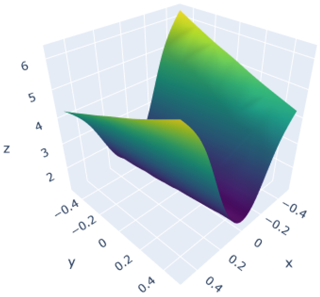
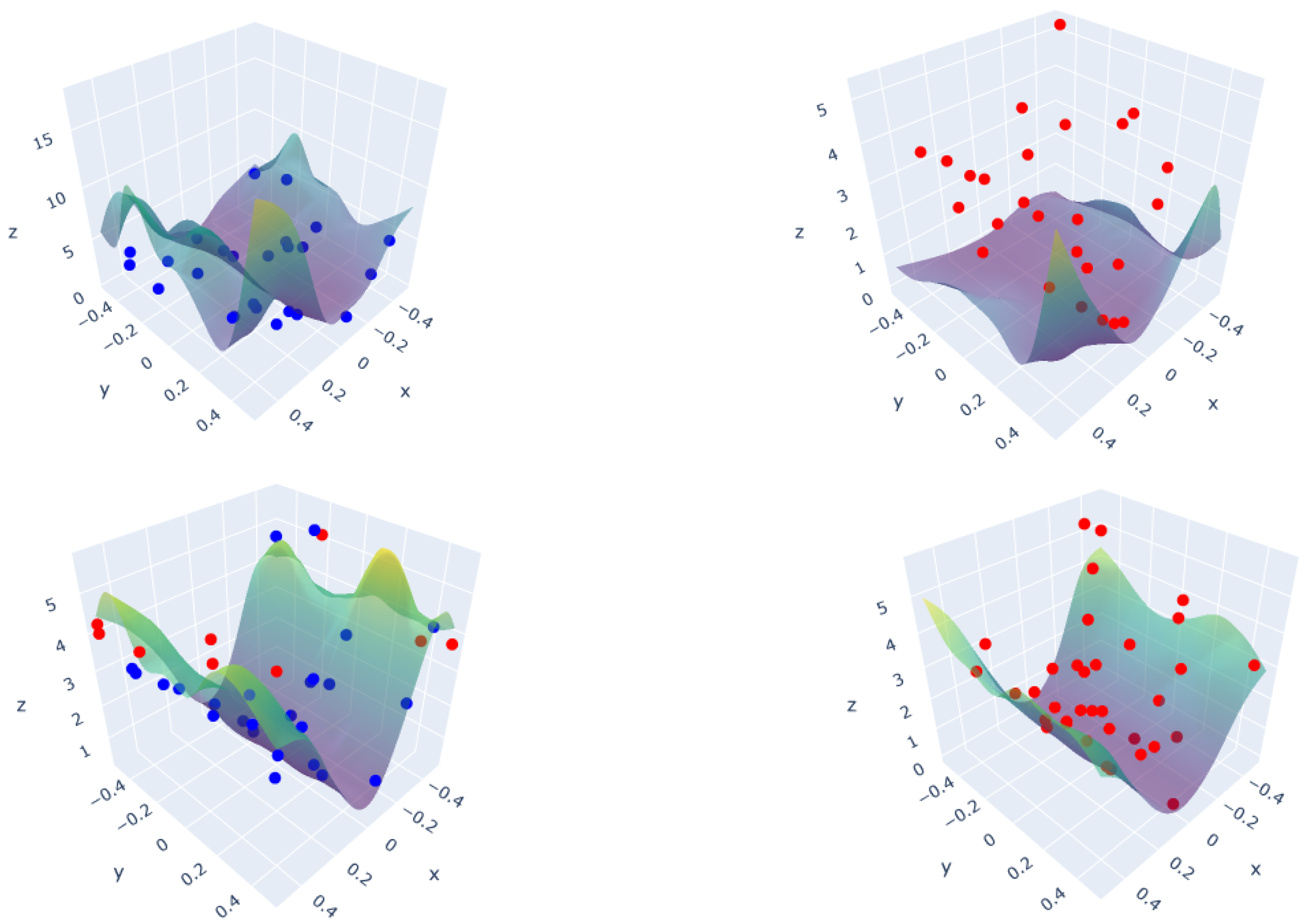
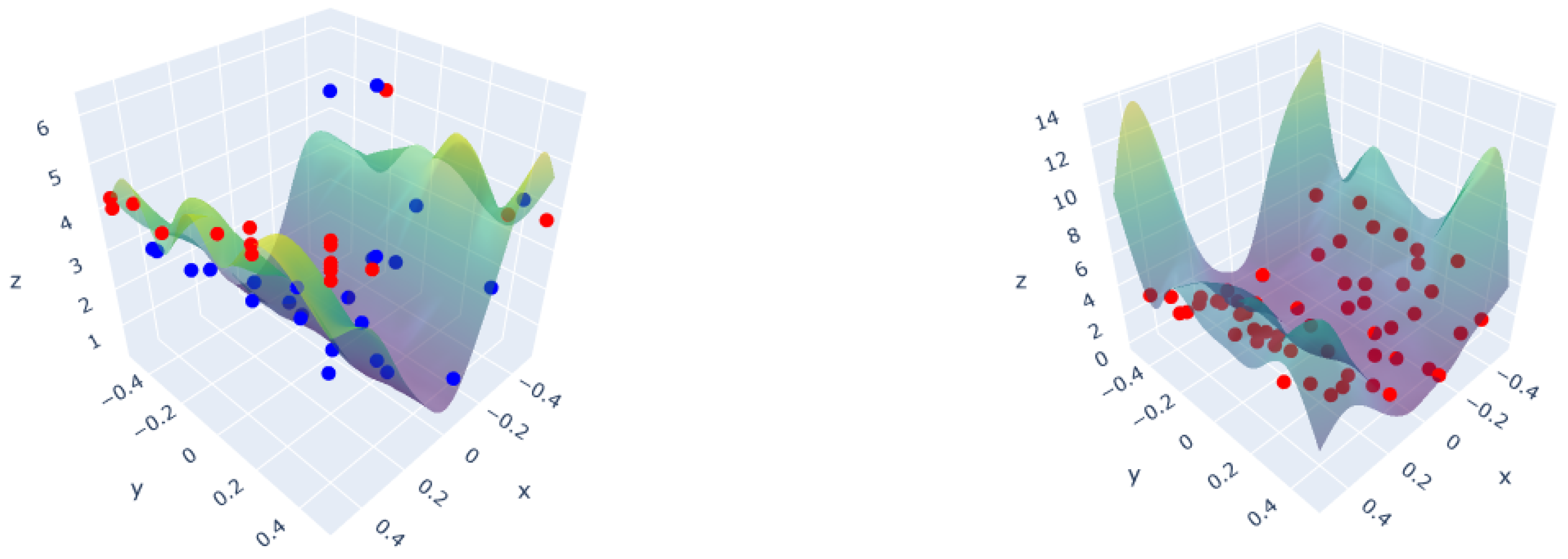
3.1. Polynomial Function

As a first example, we are trying to estimate the following polynomial function from [39] in a 5-dimensional input space.
f ( x = ( x 1 , x 2 , x 3 , x 4 , x 5 ) ) = ( 8 x 1 3 6 x 1 0.5 x 2 ) 2 + ( 4 x 3 3 3 x 3 0.25 x 4 ) 2 + 0.1 ( 2 x 5 2 1 ) .
In Figure 2, a plot of the ground truth function is shown for f ( x 1 , x 2 , x 3 = 0 , x 4 = 0 , x 5 = 0.7071 ) , as in [39], for comparison purposes.
The function is defined on the domain Ω = [ 0.5 , 0.5 ] 5 , and the predictions are made over this space using an s-PGD model trained with the Fisher matrix active learning method. The results are compared with s-PGD trained on an LHS with the same number of samples as the active method at the considered step. They are also compared with the results of the previous article [39], which were obtained through a 4th order MAS s-PGD, and an LHS of 160 points as the training set.
For the training, the s-PGD hyperparameters (modes and degrees) are set to avoid over-fitting and have good generalization. The value of R² on the training set is constant and around 0.8.
Moreover, for the matrix method, the next sample is chosen within a pool of available samples, like in a pool-based strategy. This pool is defined as a k-dimensional grid (five here) of N subdivisions, which gives a group of N k possible elements evenly distributed over the input parametric space. In our application, a refined research grid of size 20 5 is used in order to have a wide choice of queries.
In Figure 3, the output shape of the function is plotted at different steps for the same fixed parameters as before. For the active method, on the plots on the left side of Figure 3, the blue dots are the initial training points for the model, and the red ones are the new added points after different numbers of queries. On the the plots on the right side of Figure 3, the samples are generated with an LHS. For each step, a new LHS is generated, with a number of samples corresponding to the number of training samples of the active method. For example, in the middle of Figure 3, we start with 25 samples (blues dots), and we add 9 queries (red dots) in the active method (so 34 training samples) and we compare with an LHS of 34 samples.
With the matrix method, the training points are added accordingly to the shape of the predicted output function and in order to reduce the output variance. This leads to more points on the curved areas and borders. While, as expected, the LHS gives a more random and evenly distributed screening on the input space independent of the output shape. As shown in Figure 3, the prediction is adapted step by step in the matrix method until there is no more significant change. This precision can be settled accurately by adapting the value of the stopping criterion.
To compare more directly the performances of both methods, the correlation coefficients, defined as follows in Equation (26) and calculated on a test set, are evaluated. The test set considered includes all the points of the grid that are not used as training. Because the grid is refined, it is assumed that it is a densely populated and evenly distributed test set that gives significant results.
R 2 = i = 1 n ( Y p r e d , i Y p r e d ¯ ) ( Y t r u e , i Y t r u e ¯ ) i = 1 n ( Y p r e d , i Y p r e d ¯ ) 2 ( Y t r u e , i Y t r u e ¯ ) 2 ,
where Y p r e d corresponds to the prediction made by the model, Y t r u e to the real output values and Y p r e d ¯ , Y t r u e ¯ to the corresponding means.
The results, from 25 to 55 queries, for both the LHS and matrix method at each step are plotted in Figure 4. These plots have been repeated for 400 iterations of the whole active learning process with different initialization databases (constructed with different LHS of 25 values). The average, first, and last quartile of R 2 have been extracted for each method.
It appears that the matrix method converges faster than the LHS, reaching a stable level with a training database of 40 samples, while the LHS performances are still increasing and lower. Adding samples increasingly gives an average correlation value of 0.824, while it only reaches 0.647 with an LHS for 35 samples. Compared with the results of the previous study in [39], where training of an LHS with 160 samples was chosen to reach an R 2 of 0.88, here the same value can be obtained with only 35 samples.
In addition, it is also noteworthy that the initial training database has a large impact on the results, especially at the beginning of the active learning process. Indeed, the interquartile range is, at first, around 0.23 for the matrix method and 0.21 for the LHS, meaning the dispersion is notable. After that, it decreases quickly for the matrix method, reaching 0.07 against 0.5 for the LHS at around 10 queries. This phenomenon is explained by the fact that the LHS seeks to increase the inertia by starting in random directions. This is optimal for a group of tests, but the estimator does not take into account the past training data. On the contrary, our approach is to seek to optimize the points and the past sets of points with a criterion of minimization of the variance. Also, for this kind of criterion, after a while adding a point has less and less impact, and the criterion become stationary. That is why a stabilization appears.
Moreover, the grid size can be more or less refined and needs a compromise. Indeed, this is illustrated in Figure 5, where the final value of R 2 after 30 queries is plotted. That is to say, after the criterion has converged and there is no more variation between the queries at the state n and n + 1 . This shows that, with a wider grid size, the R 2 values obtained by the matrix method can be higher and thus the performances obtained by the model are better. For example, for 35 queries, an R 2 value of 0.790 is obtained for a 10 5 grid against 0.824 for a 20 5 grid.
This can be easily explained because, with a more refined grid, more “next points” are available, and the algorithm can choose more precisely where to add a new point. However, it is also more time-consuming to compute the criterion for the whole grid, and it is more memory consuming to save and calculate the corresponding values. Thus, a compromise is necessary. Moreover, it appears in Figure 5 that after 10 subdivisions the slope of increase is lower. For this problem, a subdivision after 10 should be chosen, still taking into account the calculation time.
Globally, the results obtained with the matrix method appear to be significantly better than with usual samplings. Although at first it is more time-consuming or computationally more expensive to determine the next point to add at each step, time and costs are saved in the end because fewer samples are required by the model to converge. This aspect is particularly interesting for industrial applications where simulation or experimental costs need to be minimized.

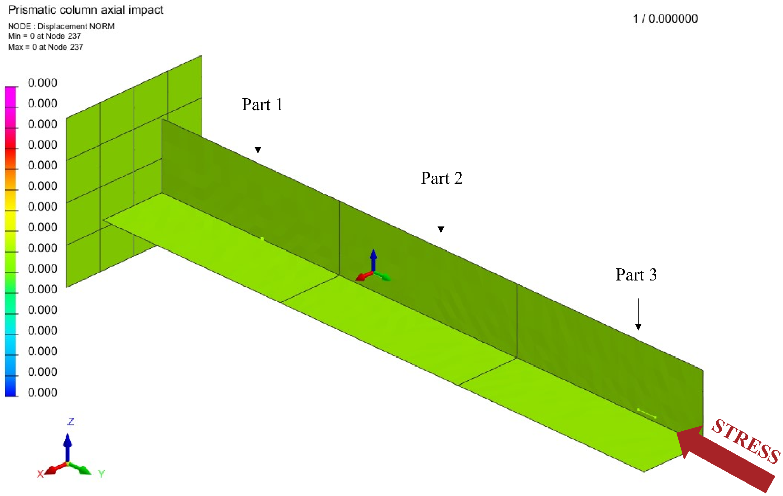
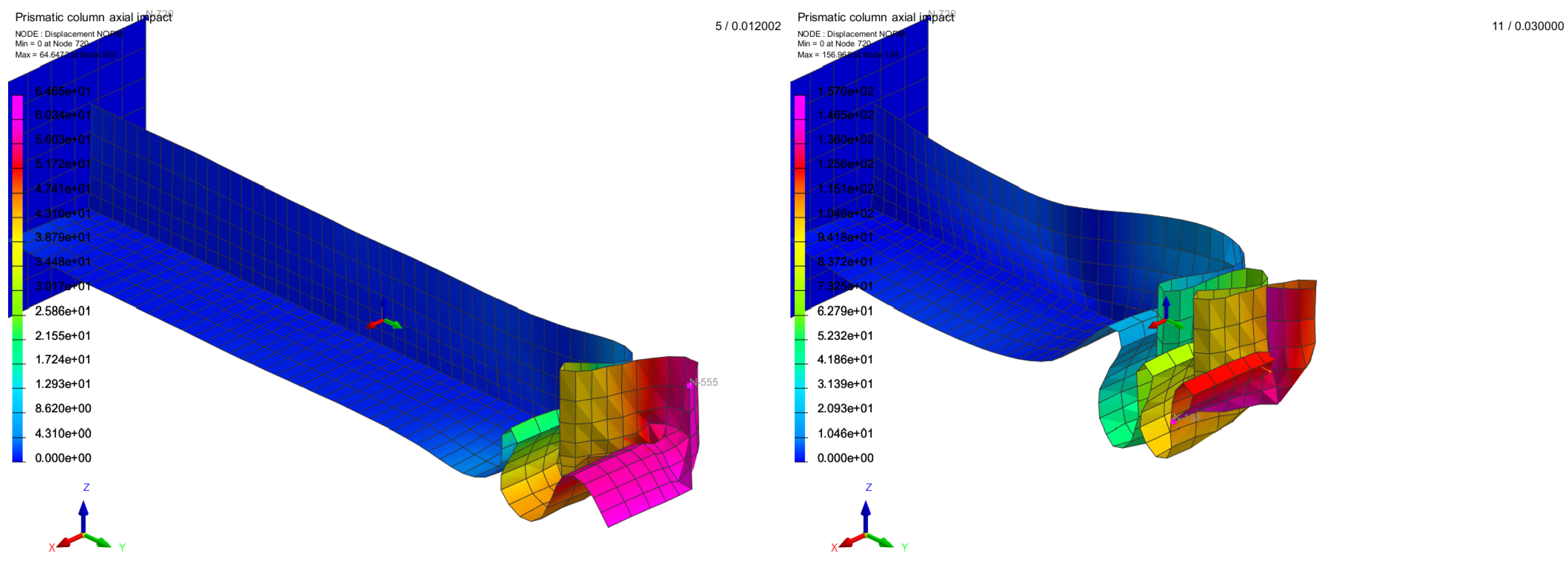
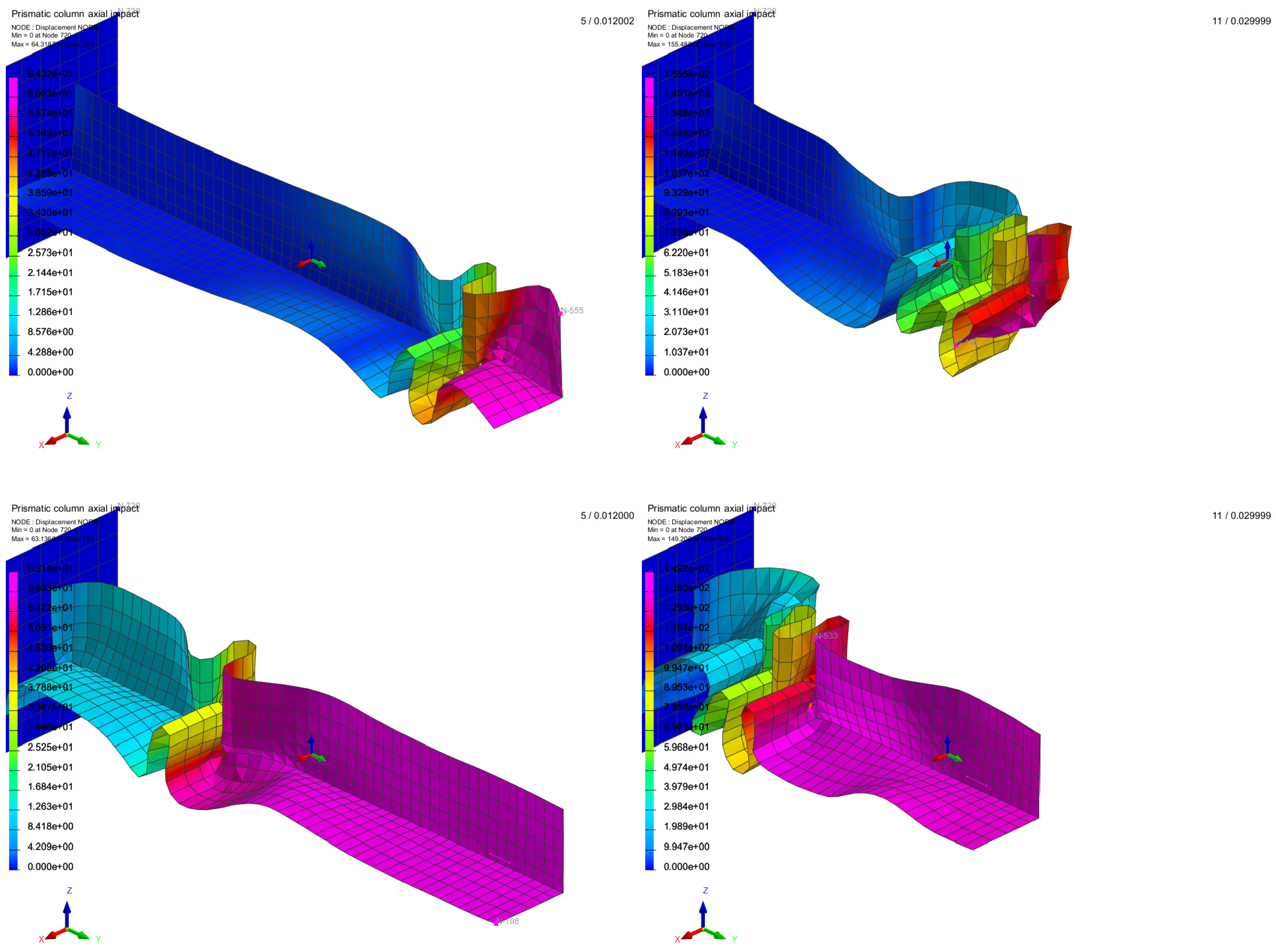
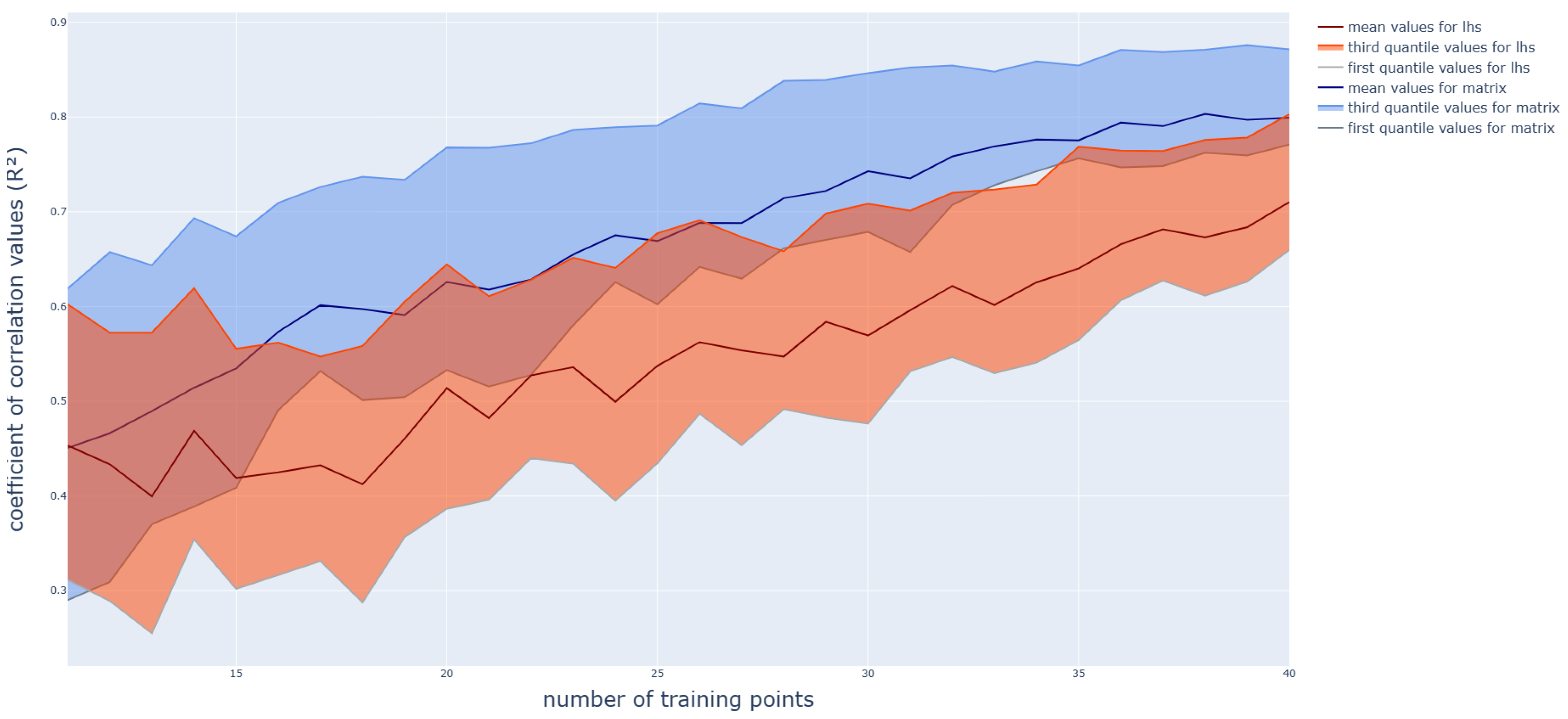
3.2. Application on a Box-Beam Crash Absorber

Now, this method was applied to an industrial mechanical problem through a box-beam deformation example. The idea here is to study and predict the deformation of a beam separated in three parts. Each part (part 1, part 2, and part 3) has a specific thickness. The whole beam is subjected to a loading along its main axis ( y ) on one side and clamped on the other. The model is represented in Figure 6.
The application of the stress smashes the beam along the y-axis. The corresponding deformation depends on the thickness chosen for the three boxes. Some cases are represented in Figure 7. The first, intermediate, and last time steps for different input values of thicknesses for the three parts are illustrated.
In this case, the model’s aim is to estimate the displacement along the main axis of a point located at the edge of the beam at the final simulation time step function of the thicknesses chosen for each box as input parameters ( h 1 , h 2 , h 3 ) . The box-beam is a classic test for computational mechanics of particular interest in the automotive industry. The simulations were carried out using the commercial the software VPS (version 2022) from ESI Group. ESI Group is considering the proposed technology addressed in the present paper within the AdMoRe ESI solver. The ranges of the thicknesses area 1 to 1.7 mm.
As before, we will compare the performances (in terms of R 2 values) for s-PGD models trained with our active method and with an LHS with the same number of training samples. As only three parameters are involved here, the initialization for the matrix method is performed with a small LHS of 10 samples.
Moreover, the whole process is repeated 100 times to produce an average of the results obtained, which is plot in Figure 8.
The grid is refined with a 3 50 size to be precise enough.
It appears in Figure 8 that, as for the previous example, the matrix method reaches higher values of R 2 faster than the use of a usual DOE. Indeed, it gives on average a value 12 % higher than with the LHS. However, the increases with the two methods are more similar here than before. The differences are also less important. This can be explained by the fact that there are only three parameters involved and the behavior of the output is quite simple. There is also still a variability associated to the initialization state, with a 19 % average variation for the matrix method and 22 % for the standard LHS.
As for this kind of criterion, where a stable level is often reached for the reasons detailed before, a stable level is probably reached but for more queries. For an industrial application, it is assumed that an R² of 0.8 is enough (regarding the computing time of those simulations). Therefore, the active method allows us to achieve good global predictions with few samples here also.

4. Conclusions and Future Works

To sum up, a new information criterion was proposed to determine which sample would be the most valuable to add to the training database of a high-dimensional regression model to improve its performances step by step. The results of this method appear to be quite conclusive. Indeed, the precision of the predictions function of the number of samples in the training database increases faster with this method than with a more usual DOE (such as LHS). Moreover, this criterion does not only depend on the shape of the input space, but also takes into account the output values. This way, the models are automatically refined where there are variations in the output space and can adapt faster to a specific problem.
However, this methodology can still be improved in different ways:
  • First, the samples in this study, are added one by one, but it could be interesting to add them by group. Indeed, it seems that the algorithm needs to select some points in the same area to estimate it before moving to others. This behavior can be explained by the fact that the information criterion used aims to minimize the global output variance. Adding points by group could be an interesting way to solve this issue. In further studies, studying how many points to add would be relevant. Moreover, when the real output value (given by the “oracle”) comes from experiments, it is more pertinent to add more than one point simultaneously to have better organization.
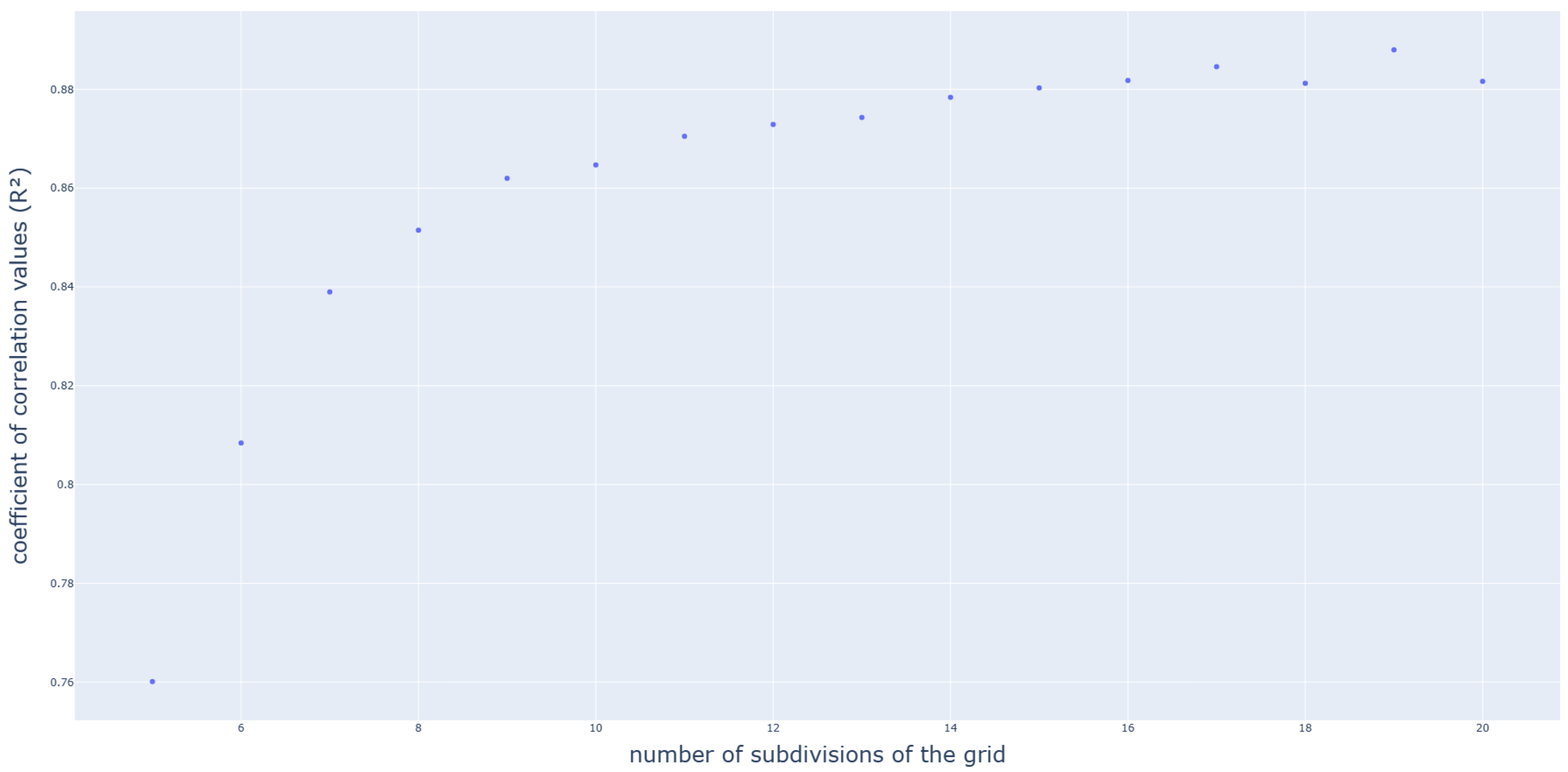
  • Another point that could be optimized is the search for the criterion optimum value. As for now, a simple search along a refined grid is used. Using an optimized method to find the optimum (such as a gradient descent for example) or using another model for the criterion could be an option. This is also interesting for the purpose of reducing the computational cost of the algorithm. Indeed, finding the optimal value without generating a huge grid would be a good improvement and should be optimized.
  • In terms of practical use, developing an algorithm to determine and maybe adapt the s-PGD parameter (number of modes, function degrees) during the whole active learning process would also improve the speed of convergence.
  • Finally, the mix of the criterion with a more specific cost function is also considered to improve the results, as was studied in the preliminary step of the method development.
In the end, let us highlight that the matrix method criterion is particularly efficient for high-dimensional problems. Indeed, unlike the usual active learning regression criterion, it does not depend on any distance. This will be confirmed by applying this new methodology for a much higher dimensional problem.

Author Contributions

Conceptualization, F.C. and M.L.; methodology, N.H. and C.G.; validation, N.H., C.G. and F.D.; investigation, F.C., M.L., N.H. and C.G.; resources, F.D.; writing—original draft preparation, C.G.; writing—review and editing, N.H., F.C. and M.L.; supervision, N.H., F.C. and M.L. All authors have read and agreed to the published version of the manuscript.

Funding

This research received no external funding.

Institutional Review Board Statement

Not applicable.

Data Availability Statement

Data supporting the findings of this study are available from the corresponding author upon reasonable request.

Conflicts of Interest

Fatima Daim is an employee of the company CNRS@CREATE Ltd. The remaining authors declare that the research was conducted in the absence of any commercial or financial relationships that could be construed as a potential conflict of interest. The authors acknowledge the contribution and support of the ESI through the contribution of Fatima Daim.

Appendix A. Matrix Method Criterion Detailed Definition

Let us consider an unknown function whose approximation is precisely the objective of this work. A function, f, depending on n input variables x 1 , x 2 , . . . , x n such as:
f ( x 1 , x 2 , . . . , x n ) : Ω R n R .
With s-PGD, it can be also written as:
f ( x 1 , . . . , x n ) f ˜ M ( x 1 , . . . , x n ) = m = 1 M k = 1 n X m k ( x k ) .
The modes will be noted m, the degrees of the functions d, and the dimensions k and X m k and N d k are the decomposition vectors.
The corresponding vector for an example where m = [ 1 , 2 ] , d = [ 1 , 2 ] and k = [ 1 , 2 , 3 ] can be written:
J ( μ , x 1 , x 2 , x 3 ) = m = 1 , d = 1 k = 1 k = 2 k = 3 N 1 1 ( x 1 ) X 1 2 ( x 2 ) X 1 3 ( x 3 ) N 1 2 ( x 1 ) X 1 2 ( x 2 ) X 1 3 ( x 3 ) N 1 3 ( x 1 ) X 1 2 ( x 2 ) X 1 3 ( x 3 ) m = 2 , d = 1 k = 1 k = 2 k = 3 N 1 1 ( x 1 ) X 2 2 ( x 2 ) X 2 3 ( x 3 ) N 1 2 ( x 1 ) X 2 2 ( x 2 ) X 2 3 ( x 3 ) N 1 3 ( x 1 ) X 2 2 ( x 2 ) X 2 3 ( x 3 ) m = 1 , d = 2 k = 1 k = 2 k = 3 X 1 1 ( x 1 ) N 2 1 ( x 2 ) X 1 3 ( x 3 ) X 1 1 ( x 1 ) N 2 2 ( x 2 ) X 1 3 ( x 3 ) X 1 1 ( x 1 ) N 2 3 ( x 2 ) X 1 3 ( x 3 ) m = 2 , d = 2 k = 1 k = 2 k = 3 X 2 1 ( x 1 ) N 2 1 ( x 2 ) X 2 3 ( x 3 ) X 2 1 ( x 1 ) N 2 2 ( x 2 ) X 2 3 ( x 3 ) X 2 1 ( x 1 ) N 2 3 ( x 2 ) X 2 3 ( x 3 )
According to the methodology seen in Section 2.4, on a considered point ( x 1 , x 2 , x 3 ) and for a model previously trained on the database, ξ , we have the criterion:
d ( μ , x 1 , x 2 , x 3 ) f ( μ , x 1 , x 2 , x 3 ) μ T I ( μ , ξ ) f ( μ , x 1 , x 2 , x 3 ) μ = J ( μ , x 1 , x 2 , x 3 ) T I ( μ , ξ ) J ( μ , x 1 , x 2 , x 3 ) .
This value, d, will be the new criterion used to determine the information in one point of the database. Therefore, it controls whether or not the point should be added to the training set.

References

  1. Mitchell, T. Machine Learning; McGraw-Hill: New York, NY, USA, 1997. [Google Scholar]
  2. Laughlin, R.B.; Pines, D. The theory of everything. Proc. Natl. Acad. Sci. USA 2000, 97, 28–31. [Google Scholar] [CrossRef] [PubMed]
  3. Goupy, J.; Creighton, L. Introduction to Design of Experiments; Dunod/L’Usine nouvelle: Paris, France, 2006. [Google Scholar]
  4. Settles, B. Active Learning Literature Survey; Computer Sciences Technical Report; University of Wisconsin-Madison: Madison, WI, USA, 2009. [Google Scholar]
  5. Frieden, B.R.; Gatenby, A.R. Principle of maximum Fisher information from Hardy’s axioms applied to statistical systems. Comput. Sci. Tech. Rep. E 2013, 88, 042144. [Google Scholar] [CrossRef]
  6. Ibáñez, R.; Abisset-Chavanne, E. A Multidimensional Data-Driven Sparse Identification Technique: The Sparse Proper Generalized Decomposition; Hindawi: London, UK, 2018. [Google Scholar]
  7. Fisher, R. The Arrangement of Field Experiments. J. Minist. Agric. Great Br. 1926, 33, 503–515. [Google Scholar]
  8. Box, G.E.; Hunter, W.G.H. Statistics for Experimenters: Design, Innovation, and Discovery; Wiley: Hoboken, NJ, USA, 2005. [Google Scholar]
  9. Plackett, R.L.; Burman, J.P. The Design of Optimum Multifactorial Experiments. Biometrika 1946, 33, 305–325. [Google Scholar] [CrossRef]
  10. McKay, M.D.; Beckman, R.J.; Conover, W.J. A Comparison of Three Methods for Selecting Values of Input Variables in the Analysis of Output from a Computer Code. Technometrics Am. Stat. Assoc. 1979, 42, 55–61. [Google Scholar]
  11. Nguyen, N.K. A new class of orthogonal Latin hypercubes. In Statistics and Applications, Volume 6, Nos.1 & 2, (New Series); Society of Statistics, Computer and Applications: New Delhi, India, 2008; pp. 119–123. [Google Scholar]
  12. Angluin, D. Queries Concept Learning. Mach.-Mediat. Learn. 1988, 2, 319–342. [Google Scholar] [CrossRef]
  13. Angluin, D. Queries Revisited; Springer: Berlin/Heidelberg, Germany, 2001. [Google Scholar]
  14. Cohn, Z.G.D.; Jordan, M. Active learning with statistical models. J. Artif. Intell. Res. 1996, 4, 129–145. [Google Scholar] [CrossRef]
  15. Atlas, L.; Cohn, D.; Ladner, R.; El-Sharkawi, M.A.; Marks, R.J. Training connection networks with queries and selective sampling. In Advances in Neural Information Processing Systems 2; Morgan Kaufmann Publishers, Inc.: San Francisco, CA, USA, 1990; pp. 566–573. [Google Scholar]
  16. Lewis, D.; Gale, W. A sequential algorithm for training text classifiers. In Proceedings of the ACM SIGIR Conference on Research and Development Information Retrieval, Dublin, Ireland, 3–6 July 1994. [Google Scholar]
  17. Lewis, D.; Catlett, J. Heterogeneous uncertainty sampling for supervised learning. In Proceedings of the International Conference on Machine Learning (ICML), New Brunswick, NJ, USA, 10–13 July 1994. [Google Scholar]
  18. Scheffer, T.; Decomain, C.; Wrobel, S. Active hidden Markov models for information extraction. In Proceedings of the International Conference on Advancesin Intelligent Data Analysis (CAIDA), Cascais, Portugal, 13–15 September 2001. [Google Scholar]
  19. Shannon, C. A mathematical theory of communication. Bell Syst. Tech. J. 1948, 27, 379–423. [Google Scholar] [CrossRef]
  20. Seung, H.S.M.O.; Sompolinsky, H. Query by committee. In Proceedings of the ACM Workshop on Computational Learning Theory, Pittsburgh, PA, USA, 27–29 July 1992. [Google Scholar]
  21. Dagan, I.; Engelson, S. Committee-based sampling for training probabilistic classifiers. In Proceedings of the International Conference on Machine Learning (ICML), Tahoe City, CA, USA, 9–12 July 1995. [Google Scholar]
  22. McCallum, A.; Nigam, K. Employing EM in pool-based active learning for text classification. In Proceedings of the International Conference on Machine Learning (ICML), Madison, WI, USA, 24–27 July 1998. [Google Scholar]
  23. Seung, H.S.M.O.; Sompolins, H. Multiple-instance active learning. Adv. Neural Inf. Process. Syst. 20 (Nips) 2007, 1289–1296. [Google Scholar]
  24. Settles, B.; Craven, M.; Friedland, L. Active learning with real annotation costs. In Proceedings of the NIPS Workshop on Cost-Sensitive Learning, Whistler, BC, Canada, 12 December 2008. [Google Scholar]
  25. MacKay, D. Information-based objective functions for active data selection. Neural Comput. 1992, 4, 590–604. [Google Scholar] [CrossRef]
  26. Gal, Y.; Riashat Islam, Z.G. Deep Bayesian Active Learning with Image Data. In Proceedings of the International Conference on Machine Learning, Sydney, Australia, 6–11 August 2017. [Google Scholar]
  27. Qu, T.; Guan, S.; Feng, Y.T.; Ma, G.; Zhou, W.; Zhao, J. Deep active learning for constitutive modelling of granular materials: From representative volume elements to implicit finite element modelling. Int. J. Plast. 2023, 164, 103576. [Google Scholar] [CrossRef]
  28. Deng, W.; Liu, Q.; Zhao, F.; Pham, D.T.; Hu, J.; Wang, Y.; Zhou, Z. Learning by doing: A dual-loop implementation architecture of deep active learning and human-machine collaboration for smart robot vision. Robot. Comuted Integr. Manuf. 2024, 86, 102673. [Google Scholar] [CrossRef]
  29. Martins, V.E.; Cano, A.; Junior, S.B. Meta-learning for dynamic tuning of active learning on stream classification. Pattern Recognit. 2023, 138, 109359. [Google Scholar] [CrossRef]
  30. Ren, M.; Triantafillou, E.; Ravi, S.; Snell, J.; Swersky, K.; Tenenbaum, J.B.; Larochelle, H.; Zemel, R.S. Meta-Learning for Semi-Supervised Few-Shot Classification. Conference paper at ICLR arXiv 2018, arXiv:1803.00676. [Google Scholar]
  31. Sousa, A.F.; Prudêncio, R.B.; Ludermir, T.B.; Soares, C. Active learning and data manipulation techniques for generating training examples in meta-learning. Neurocomputing 2016, 194, 45–55. [Google Scholar] [CrossRef]
  32. Wu, X.; Xiao, L.; Sun, Y.; Zhang, J.; Ma, T.; He, L. A survey of human-in-the-loop for machine learning. Future Gener. Comput. Syst. 2022, 135, 364–381. [Google Scholar] [CrossRef]
  33. Atkinson, A.; Donev, A.; Tobias, R. Optimum experimental designsock. In SAS; OUP: Oxford, UK, 2007; Volume 34. [Google Scholar]
  34. Mitchell, T.J. An algorithm for the construction of “D-optimal” experimental designs. Technometrics 2000, 42, 48–54. [Google Scholar]
  35. Wilmut, M.; Zhou, J. D-optimal minimax design criterion for two-level fractional factorial designs. J. Stat. Plan. Inference 2011, 141, 576–587. [Google Scholar] [CrossRef]
  36. Zhang, Q.Z.; Dai, H.S.; Liu, M.Q.; Wang, Y. A method for augmenting supersaturated designs. J. Stat. Plan. Inference 2019, 199, 207–218. [Google Scholar] [CrossRef]
  37. Lu, L.; Anderson-Cook, C.M. Input-response space-filling designs. Qual. Reliab. Eng. Int. 2021, 37, 3529–3551. [Google Scholar] [CrossRef]
  38. Chinesta, F.; Huerta, A.; Rozza, G.; Willcox, K. Encyclopedia of Computational Mechanics; Volume Model Order Reduction; John Wiley and Sons: Hoboken, NJ, USA, 2015. [Google Scholar]
  39. Sancarlos, A.; Victor Champaney, J.L.D.; Chinesta, F. PGD-based Advanced Nonlinear Multiparametric Regression for Constructing Metamodels at the scarce data limit. arXiv 2021, arXiv:2103.05358. [Google Scholar]
  40. Ibanez, R. Advanced Physics-Based and Data-Driven Strategies. Ph.D. Thesis, Universitat Politècnica de Catalunya · Barcelona Tech—UPC, Barcelona, Spain, 2019. [Google Scholar]
  41. Sancarlos, A.; Cueto, E.; Chinesta, F.; Duval, J.L. A novel sparse reduced order formulation for modeling electromagnetic forces in electric motors. SN Appl. Sci. 2021, 3, 355. [Google Scholar] [CrossRef]
  42. Sancarlos, A.; Cameron, M.; Abel, A.; Cueto, E.; Duval, J.-L.; Chinesta, F. From ROM of electrochemistry to ai-based battery digital and hybrid twin. Arch. Comput. Methods Eng. 2020, 28, 979–1015. [Google Scholar] [CrossRef]
  43. Argerich, C. Study and Development of New Acoustic Technologies for Nacelle Products. Ph.D. Thesis, Universitat Politecnica de Catalunya, Barcelona, Spain, 2020. [Google Scholar]
  44. RA, F. On the mathematical foundations of theoretical statistics. A Contain. Pap. Math. Phys. Character 1922, 222, 309–368. [Google Scholar]
  45. Kiefer, J.; Wolfowitz, J. The equivalence of two extremum problems. Can. J. Math. 1960, 12, 363–366. [Google Scholar] [CrossRef]
Figure 1. Active learning detailed methodology.
Computation 12 00024 g001
Figure 2. Ground truth for f ( x 1 , x 2 , x 3 = 0 , x 4 = 0 , x 5 = 0.7071 ) .
Computation 12 00024 g002
Figure 3. Predictions with the matrix method (left) and a classic LHS (right) for x 1 , x 2 , x 3 = 0 , x 4 = 0 , x 5 = 0.7071 after 0 (top), 9 (middle), and 29 (bottom) queries.
Computation 12 00024 g003aComputation 12 00024 g003b
Figure 4. Evolution of R² values for the two methods as a function of the number of points in the training set over 400 runs of the whole active learning process.
Computation 12 00024 g004
Figure 5. Impact of the grid size on the performances of the matrix method.
Computation 12 00024 g005
Figure 6. Structure of the box-beam and settlement of the problem.
Computation 12 00024 g006
Figure 7. Visualisation of 3D box-beam simulation results at an intermediate and at last time steps for different input values of thicknesses for the three parts.
Computation 12 00024 g007aComputation 12 00024 g007b
Figure 8. Evolution of R² values for the two methods as a function of the number of points in the training set over 100 runs of the whole active learning process with and without active learning.
Computation 12 00024 g008
Disclaimer/Publisher’s Note: The statements, opinions and data contained in all publications are solely those of the individual author(s) and contributor(s) and not of MDPI and/or the editor(s). MDPI and/or the editor(s) disclaim responsibility for any injury to people or property resulting from any ideas, methods, instructions or products referred to in the content.

