Article

MSVR & Operator-Based System Design of Intelligent MIMO Sensorless Control for Microreactor Devices

Department of Electrical and Electronic Engineering, Graduate School of Engineering, Tokyo University of Agriculture and Technology, 2-24-16 Nakacho, Koganei-shi 184-8588, Tokyo, Japan
*
Author to whom correspondence should be addressed.
Computation 2024, 12(1), 2; https://doi.org/10.3390/computation12010002
Submission received: 30 October 2023 / Revised: 29 November 2023 / Accepted: 13 December 2023 / Published: 25 December 2023
(This article belongs to the Special Issue 10th Anniversary of Computation—Computational Engineering)

Abstract

:
Recently, microreactors, which are tubular reactors capable of fast and highly efficient chemical reactions, have attracted attention. However, precise temperature control is required because temperature changes due to reaction heat can cause reactions to proceed differently from those designed. In a previous study, a single-input/output nonlinear control system was proposed using a model in which the microreactor is divided into three regions and the thermal equation is formulated considering the temperature gradient, but it could not control two different temperatures. In this paper, a multi-input, multi-output nonlinear control system was designed using operator theory. On the other hand, when the number of parallel microreactors is increased, a sensorless control method using M–SVR with a generalized Gaussian kernel was incorporated into the MIMO nonlinear control system from the viewpoint of cost reduction, and the effectiveness of the proposed method was confirmed via experimental results.

1. Introduction

A microreactor is a tube-type reactor with a reaction capacity of about microliters. The advantages of microreactors include the ability to achieve fast and highly efficient chemical reactions due to the large surface area per unit volume and the ability to safely handle chemical reactions that may cause explosions or generate hazardous substances because the reaction volume is much smaller than that of batch reaction systems. On the other hand, precise temperature control is essential because temperature changes due to the heat of chemical reactions can cause chemical reactions that are not intended in the design. In this study, a Peltier element, one of the thermoelectric conversion elements, is used to achieve vibration-free and precise temperature control. Peltier elements have the property of heat pumps, in which a high-temperature surface and a low-temperature surface are generated when an electric current is applied, and heat is transferred from the low-temperature surface to the high-temperature surface [1,2].
The Peltier elements, microreactors, and heat spreaders used in this study, which are cooling auxiliary mechanisms, have uncertainties due to the difficulty of accurately describing their models, and therefore must be controlled to account for them. To solve this problem, research [3] on methods for the robust design of parallel compensators for non-ASPR plants with structured uncertainties has been conducted. While sliding mode control is well known as a nonlinear control theory [4,5,6,7], this study uses operator theory, which can design robust and stable controllers for nonlinear systems [8,9]. As a study using operator theory, a nonlinear temperature control system has been designed for an aluminum plate with a Peltier device that has uncertainty [10]. In recent years, due to the popularity of AI research [11,12,13,14,15,16,17,18,19], research combining operator theory and AI has also been conducted. In addition, research on multi-input/output systems, such as research on a two-dimensional direction-of-arrival estimation using a polarization rectangular array under multipath propagation [20], has attracted much attention and has been actively studied in operator theory. As an example of combined research, a study on the multi-input/output tip position control of a 3-DOF soft actuator with uncertainty proposes a method of uncertainty compensation using M–SVR, a type of machine learning, and the control of multi-input/output systems using operator theory [21]. Operator theory has also been applied to a variety of other control objects [22,23,24,25].
In addition, the output estimates of observers designed using uncertain models deviate significantly from the real values due to modeling errors. Therefore, a study on a real-time estimation filter robust to the viscoelasticity of articulated arms in motion has been reported by considering and quantitatively evaluating an uncertain articulated arm viscoelasticity model with measurement error [26]. It was also extended to a practical filter algorithm for estimating the articulated viscoelasticity of human arms using a generalized Gaussian distribution [27].
Based on the above, the objectives of this study are twofold. The first is to realize a multi-input/output temperature control system to enable control of two temperatures within a microreactor. The second is to realize sensorless control in order to solve the increase in the number of sensors caused by numbering-up (a production method in which the number of microreactors is increased and parallelized in order to achieve mass production). Since the model of microreactors includes uncertainty, a machine learning model, M–SVR, is used as an estimator in this study. M–SVR is a machine learning method that extends SVR, which is a multiple-input, single-output method, to multiple outputs. M–SVR can consider effects among outputs compared with general SVR, and M–SVR has the advantage that the number of hyperparameters does not increase as the number of outputs increases [28,29]. Furthermore, to obtain higher generalization performance than the RBF kernel in offline learning, we design a sensorless control system with a model using a generalized Gaussian kernel. On the other hand, since the generalized Gaussian kernel increases the number of parameters to be tuned compared with the RBF kernel and makes it difficult to tune to the optimal parameters, a real-coded genetic algorithm [30,31] is used for parameter tuning to efficiently search for the optimal parameters. The effectiveness of these results is confirmed via simulations and experiments on actual equipment.
This section describes the structure of this paper. Section 2 describes the experimental apparatus used in this study, its mathematical modeling, and modeling using M–SVR. Section 3 describes the design of the multi-input multi-output temperature control system and the sensorless control system using M–SVR, based on the modeling in Section 2. Section 4 describes the results of the simulation and actual machine experiments using the control system designed in Section 3, verifies the effectiveness of the proposed method, and concludes in Section sec:conclusion.

2. Modeling

As shown in Figure 1, the microreactor and heat spreader are modeled by dividing them into three regions and formulating the thermal equations for each. Let Part A 1 , Part A 2 , and Part A 3 be the areas to the left of the heat spreader and Part W 1 , Part W 2 , and Part W 3 be the areas to the left of the microreactor, where S n represents the area, and the values are shown in Table 1. The parameters used for modeling are shown in Table 2. Here, Peltier elements are installed on both sides of Part A 1 and Part A 3 .

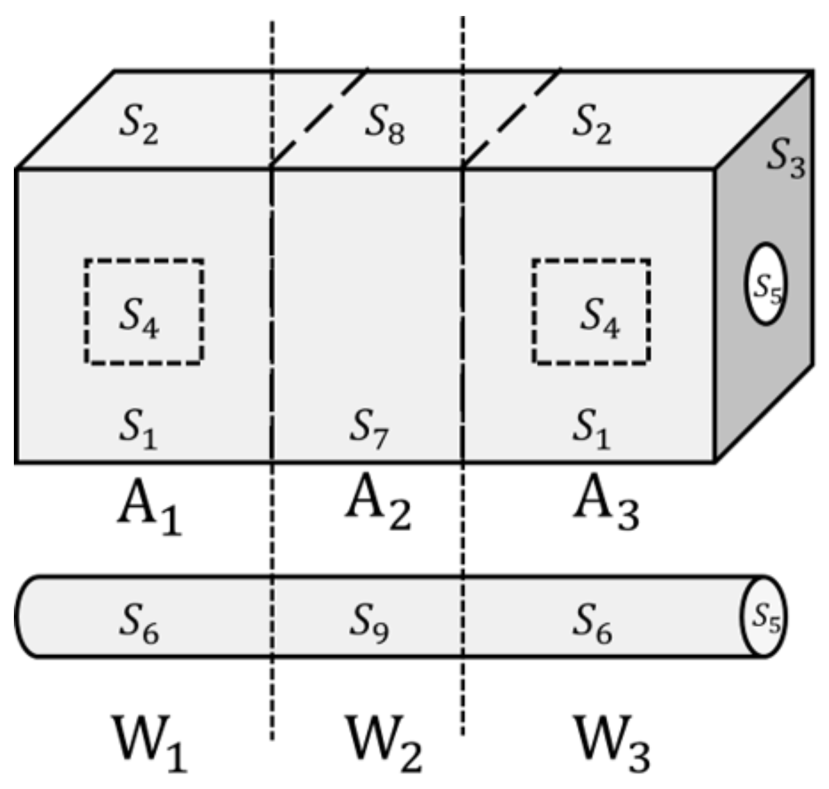
2.1. Modeling of Heat Spreader

This section models heat spreaders.
Part A 1 : d ( T 0 T a 1 ) m a 1 c a d t = 2 u d 1 α ( T 0 T a 1 ) ( 2 S 1 + 2 S 2 + S 3 S 5 ) +   α ω S 6 ( T a 1 T ω 1 ) + λ a S 3 ( T a 1 T a 2 ) d x +   ϵ a σ ( T a 1 4 T 0 4 ) ( 2 S 1 + 2 S 2 + S 3 S 5 )
Part A 2 : d ( T 0 T a 2 ) m a 2 c a d t = α ( T 0 T a 2 ) ( 2 S 7 + 2 S 8 ) + α ω S 9 ( T a 2 T ω 2 )   λ a S 3 ( T a 1 T a 2 ) d x λ a S 3 ( T a 3 T a 2 ) d x +   ϵ a σ ( T a 2 4 T 0 4 ) ( 2 S 7 + 2 S 8 )
Part A 3 : d ( T 0 T a 3 ) m a 3 c a d t = 2 u d 2 α ( T 0 T a 3 ) ( 2 S 1 + 2 S 2 + S 3 S 5 ) +   α ω S 6 ( T a 3 T ω 3 ) + λ a S 3 ( T a 3 T a 2 ) d x +   ϵ a σ ( T a 3 4 T 0 4 ) ( 2 S 1 + 2 S 2 + S 3 S 5 )
If the variables are defined as y a n = T 0 T a n ( n = 1 , 2 , 3 ) , Part A n can be expressed by Equations (4)–(6).
Part A 1 : d y a 1 d t = ω a 1 + A a 11 y a 1 + A a 12 y a 1 2 + A a 13 y a 1 3 + A a 14 y a 1 4 + λ a S 3 y a 2 m a 1 c a d x
Part A 2 : d y a 2 d t = ω a 2 + A a 21 y a 2 + A a 22 y a 2 2 + A a 23 y a 2 3 + A a 24 y a 2 4 λ a S 3 ( y a 1 + y a 3 ) m a 2 c a d x
Part A 3 : d y a 3 d t = ω a 3 + A a 31 y a 3 + A a 32 y a 3 2 + A a 33 y a 3 3 + A a 34 y a 3 4 + λ a S 3 y a 2 m a 3 c a d x
In this case, ω a n are as follows:
ω a 1 = 2 u d 1 + α w S 6 y w 1 m a 1 c a , ω a 2 = α w S 9 y w 2 m a 2 c a , ω a 3 = 2 u d 1 + α w S 6 y w 3 m a 3 c a
And A a n m are as follows:
A a 11 = ( α + 4 ϵ a σ T 0 3 ) ( S 1 + S 2 + S 3 2 S 4 S 5 ) + α w S 6 + λ a S 3 d x m a 1 c a , A a 12 = 6 ϵ a σ T 0 2 ( S 1 + S 2 + S 3 2 S 4 S 5 ) m a 1 c a , A a 13 = 4 ϵ a σ T 0 ( S 1 + S 2 + S 3 2 S 4 S 5 ) m a 1 c a , A a 14 = ϵ a σ ( S 1 + S 2 + S 3 2 S 4 S 5 ) m a 1 c a , A a 21 = ( α + 4 ϵ a σ T 0 3 ) ( 2 S 7 + 2 S 8 ) + α w S 9 + 2 λ a S 3 d x m a 2 c a , A a 22 = 6 ϵ a σ T 0 2 ( 2 S 7 + 2 S 8 ) m a 2 c a , A a 23 = 4 ϵ a σ T 0 ( 2 S 7 + 2 S 8 ) m a 2 c a , A a 24 = ϵ a σ ( 2 S 7 + 2 S 8 ) m a 2 c a , A a 31 = ( α + 4 ϵ a σ T 0 3 ) ( S 1 + S 2 + S 3 2 S 4 S 5 ) + α w S 6 + λ a S 3 d x m a 3 c a ,
A a 32 = 6 ϵ a σ T 0 2 ( S 1 + S 2 + S 3 2 S 4 S 5 ) m a 3 c a , A a 33 = 4 ϵ a σ T 0 ( S 1 + S 2 + S 3 2 S 4 S 5 ) m a 3 c a ,
A a 34 = ϵ a σ ( S 1 + S 2 + S 3 2 S 4 S 5 ) m a 3 c a

2.2. Modeling of Microreactor

In this section, we model the tubes.
Part W 1 : d ( T 0 T ω 1 ) m ω c ω d t = λ ω S 5 ( ( T ω 0 T ω 1 ) ( T ω 0 T ω 2 ) ) d x +   α ω S 6 ( T ω 1 T a 1 )
Part W 2 : d ( T 0 T ω 2 ) m ω c ω d t = λ ω S 5 ( 2 ( T ω 0 T ω 2 ) ( T ω 0 T ω 1 ) ( T ω 0 T ω 3 ) ) d x +   α ω S 9 ( T ω 2 T a 2 )
Part W 3 : d ( T 0 T ω 3 ) m ω c ω d t = λ ω S 5 ( ( T ω 0 T ω 3 ) ( T ω 0 T ω 2 ) ) d x +   α ω S 6 ( T ω 3 T a 3 )
If the variables are defined as y w k = T 0 T w k ( k = 1 , 2 , 3 , ) , Part W k can be expressed by Equations (10)–(12).
Part W 1 : d y ω 1 d t = ω ω 1 A ω 1 y ω 1 + λ ω S 5 y ω 2 m w 1 c w d x
Part W 2 : d y ω 2 d t = ω ω 2 A ω 2 y ω 2 + λ ω S 5 ( y ω 1 + y ω 3 ) m w 2 c w d x
Part W 3 : d y ω 3 d t = ω ω 3 A ω 3 y ω 3 + λ ω S 5 y ω 2 w 3 c w d x
In this case, ω w k and A a w k are as follows:
ω w 1 = α w S 6 y a 1 m w 1 c w , ω w 2 = α w S 9 y a 2 m w 2 c w , ω w 3 = α w S 6 y a 3 m w 3 c w
A w 1 = λ w S 5 d x + α w S 6 m w 1 c w , A w 2 = λ w S 5 d x + α w S 9 m w 2 c w , A w 3 = λ w S 5 d x + α w S 6 m w 3 c w

2.3. Modeling via M–SVR

To estimate the temperature of a microreactor, this section uses training data to build a model using M–SVR. M–SVR is a machine learning method that extends SVR to multiple outputs and has the advantage over general SVR of being able to consider the effects between outputs. Another advantage is that the number of hyperparameters does not increase as the number of outputs increases [28,29]. The theory of M–SVR is presented in Appendix B. In this study, a generalized Gaussian kernel is used to achieve higher generalization performance than the RBF kernel. The generalized Gaussian kernel is a kernel based on the generalized Gaussian distribution and has the property of changing the shape of the distribution with the value of the shape parameter [26]. The theory of generalized Gaussian kernels is presented in Appendix C. Three features, the currents i 1 and i 2 flowing in the Peltier element and T a 2 , the temperature of aluminium, are used as training data for the input of M–SVR, and five features, T w 1 , T a 1 , and T a 3 , the temperature of the microreactor, and T a 1 and T a 2 , the temperature of aluminium, are used as training data for the output. The training data are obtained by applying a constant current to currents i 1 and i 2 in 15 combinations obtained from 0, 100, 200, and 400 mA for 500 s each to obtain the temperatures T w 1 , T w 2 , and T w 3 of the microreactor and T a 1 , T a 2 , and T a 3 of the aluminium. The 100 samples of data obtained from each current combination were summed to obtain 1500 samples of data, which were used as training data to create the model. Hyperparameter optimization using a real-coded genetic algorithm [30] with 50 generations and 20 individuals, ranking selection as the selection method, and SPX crossover [31] as the crossover method, using the training data obtained in the experiment, and manually adjusted results are shown in Table 3 and Table 4, and MSE values in Table 5. Note that the manual adjustment is a trial-and-error adjustment made to obtain a good evaluation value using the parameters obtained by the real-valued genetic algorithm as a base point. The results show that the generalized Gaussian kernel is more accurate than the RBF kernel, so the M–SVR model with the generalized Gaussian kernel is used in this study.

3. Control Design

When performing MIMO temperature control, it is necessary to consider the coupling elements that occur between each control system. In this study, the coupling elements are separated based on the literature [8], and the two-input, two-output control system is divided into two independent subsystems for control. The theory is described in Appendix A.

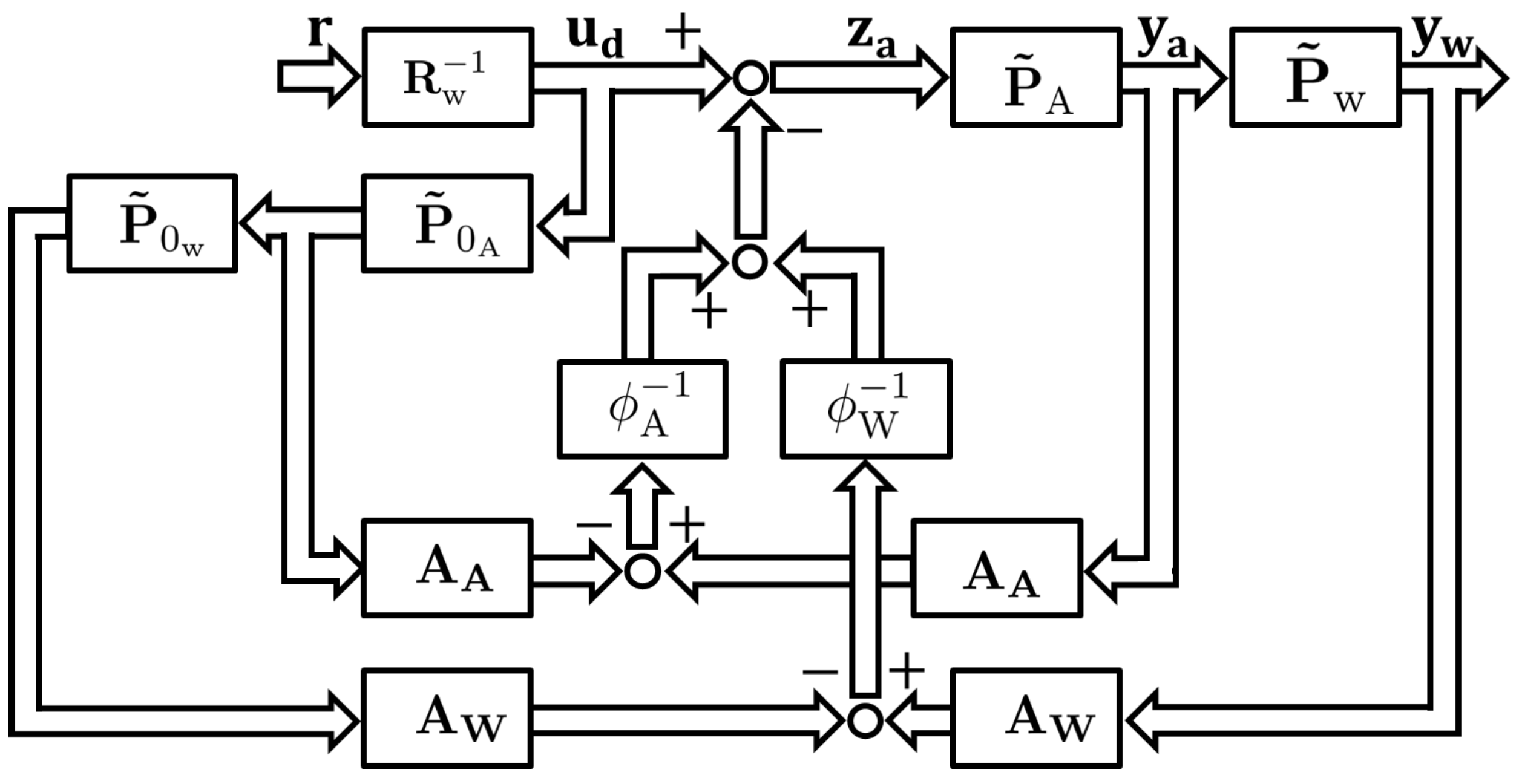
3.1. Right Factorization

Using the model derived in Section 2.1 and Section 2.2, we perform a right factorization based on operator theory. First, from Equations (4)–(6) and (10)–(12), we have that
ω a n = z a n m a n c a , ω w k = z w k m w k c w
P a r t A n : y ˙ a n = z a n m a n c a A a n 1 y a n + A a n 2 y a n 2 A a n 3 y a n 3 + A a n 4 y a n 4
P a r t W k : y ˙ w k = z w k m w k c w A w k y w k
is expressed as follows.
In this case, z a n and z w k are the input signals of processes P A n and P W k , respectively. In addition, y a n and y w k are the outputs of processes P A n and P W k , respectively. Here, z a n and z w k are expressed as follows.
z a n = 2 u d 1 + G a y a 2 + G a w y w 1 ( n = 1 ) G a y a 1 + G a y a 3 + G a w 2 y w 2 ( n = 2 ) 2 u d 2 + G a y a 2 + G a w y w 3 ( n = 3 )
z w k = G a w y a 1 + G w y w 2 ( k = 1 ) G a w 2 y a 2 + G w ( y w 1 + y w 3 ) ( k = 2 ) G a w y a 3 + G w y w 2 ( k = 3 )
Note that G a , G w , G a w , G a w 2 , G s a , and G s w are as follows.
G a = λ a S 3 d x , G w = λ w S 5 d x , G a w = α w S 6 G a w 2 = α w S 9 , G s a = 2 λ a S 3 d x , G s w = 2 λ w S 5 d x
The output-to-output coupling factors for each process are then as follows, where H a = λ a S 3 m a c a d x , H w = λ a S 5 m w c w d x .
H a 12 = H a y a 2 , H a 13 = 0 , H a 21 = H a y a 1
H a 23 = H a y a 3 , H a 31 = 0 , H a 32 = H a y a 2 H w 12 = H w y a 2 , H w 13 = 0 , H w 21 = H w y a 1
H w 23 = H w y a 3 , H w 31 = 0 , H w 32 = H w y a 2
The right factorization of each process is based on operator theory. Therefore, we represent each operator using a spatial representation as follows.
D a n 1 : z a n ( t ) ω a n ( t ) : ω a n = z a n m a n c a
N a n : ω a n ( t ) y a n ( t ) : x ˙ a n = ω a n A a n 1 y a n + A a n 2 y a n 2 A a n 3 y a n 3 + A a n 4 y a n 4 y a n = x a n

3.2. Without Interference Effects

Figure 2 shows the control system for eliminating the effects of interference.
In this case, P ˜ A = ( P ˜ A 1 , P ˜ A 2 , P ˜ A n ) , P ˜ A n = N A n R A n 1 , P ˜ W = ( P ˜ W 1 , P ˜ W 2 , P ˜ W n ) , P 0 ˜ A = ( P 0 ˜ A 1 , P 0 ˜ A 2 , P 0 ˜ A n ) , and P 0 ˜ W = ( P 0 ˜ W 1 , P 0 ˜ W 2 , P 0 ˜ W n ) . P 0 ˜ A = ( P 0 ˜ A 1 , P 0 ˜ A 2 , P 0 ˜ A n ) is the thermal model of the heat spreader, and P 0 ˜ W = ( P 0 ˜ W 1 , P 0 ˜ W 2 , P 0 ˜ W n ) is the tube thermal model. P 0 ˜ A can undergo right factorization as follows.
P 0 ˜ A n = N A 0 n R A n 1 N 0 A n N A n
Also, ϕ A = ( ϕ A 1 , ϕ A 2 , ϕ A n ) and ϕ W = ( ϕ W 1 , ϕ W 2 , ϕ W n ) are linear operators such that ϕ i ( α ( t ) ) 0 for any bounded α ( t ) . Here, the effect of interference can be eliminated by designing the control system so that the interference term is equal to the feedback term, as shown in the following equation. Each operator is designed with A A = I , A W = I , ϕ A i 1 ( α i ) ( t ) = 1 n a α i , ϕ W i 1 ( α i ) ( t ) = 1 n w α i , where α i is the bounded signal and n a and n w are design parameters.
z i ( t ) = u d i + d i ( t ) + ϕ A i 1 A A i P ˜ 0 A i ( u d i ) ( t ) +   ϕ W i 1 A W i P ˜ 0 W i P ˜ 0 A i ( u d i ) ( t )   ϕ A i 1 A A i P ˜ A i ( z i ) ( t ) ϕ W i 1 A W i P ˜ W i P ˜ A i ( z i ) ( t )
Transform the equation for z i ( t ) .
ϕ A i 1 ( ϕ A i + A A i P ˜ A i ) ( z i ) ( t ) + ϕ W i 1 ( ϕ W i + A W i P ˜ W i P ˜ A i ) ( z i ) ( t ) = d i ( t ) + ϕ A i 1 ( ϕ A i + A A i P 0 ˜ A i ) ( u d i ) ( t ) +   ϕ W i 1 ( ϕ W i + A W i P 0 ˜ W i P 0 ˜ A i ) ( u d i ) ( t )
From the above equation, the input signal z i ( t ) equals the output u i ( t ) of operator B 1 .
z i ( t ) u d i ( t )

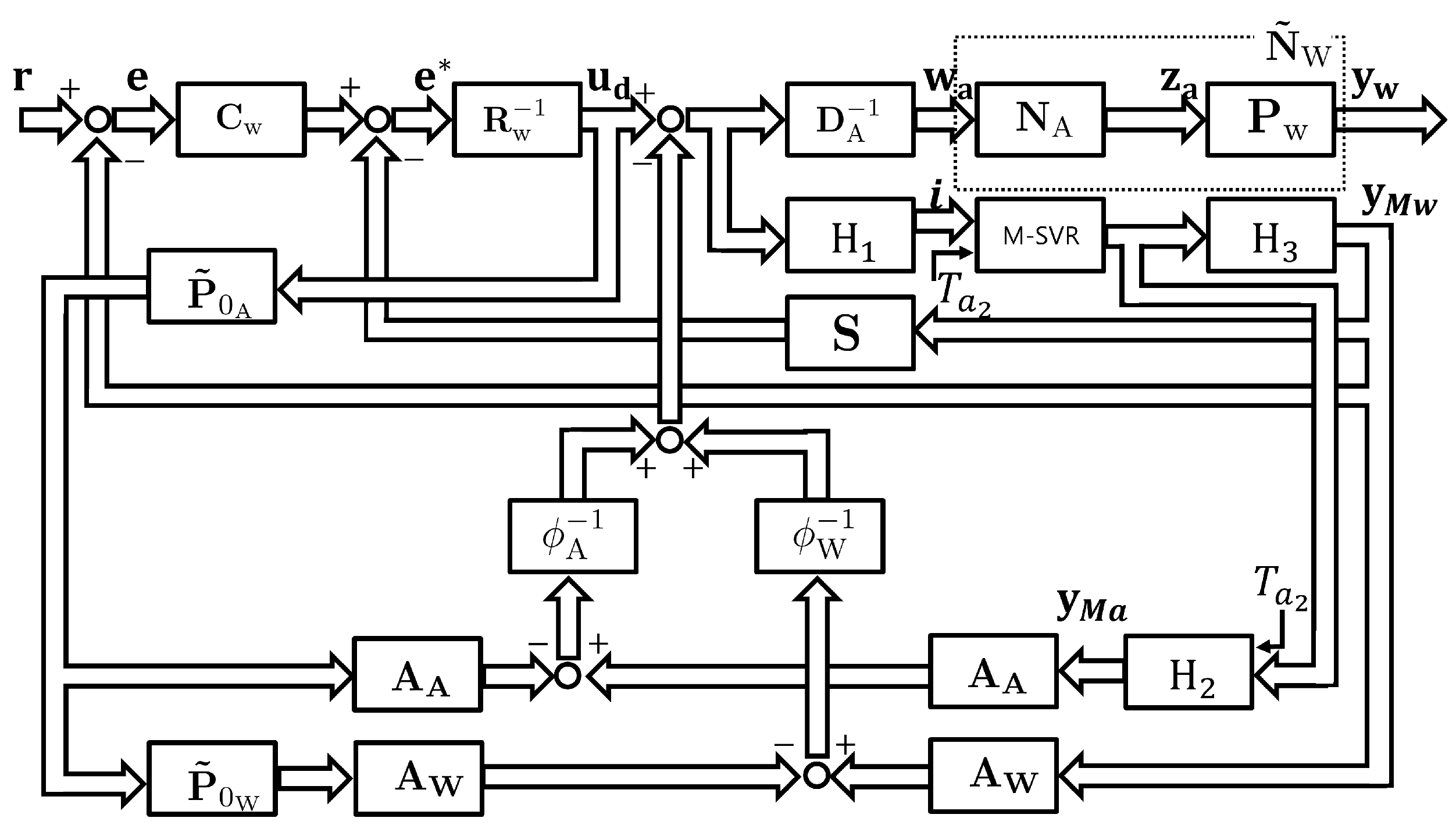
3.3. Controller Design

The control system designed based on operator theory is shown in Figure 3. In this case, each plant is D A = ( D A 1 , D A 2 , D A n ) , N A = ( N A 1 , N A 2 , N A n ) , and P W = ( P W 1 , P W 2 , P W n ) , and the controllers are S = ( S 1 , S 2 , S n ) , R W = ( R W 1 , R W 2 , R W n ) , and C W = ( C W 1 , C W 2 , C W n ) . Also, each signal is e * = ( e 1 * , e 2 * , e n * ) , e = ( e 1 , e 2 , e n ) , r = ( r 1 , r 2 , r n ) , u d = ( u d 1 , u d 2 , u d n ) , w a = ( w a 1 , w a 2 , w a n ) , y a = ( y a 1 , y a 2 , y a n ) , and y = ( y 1 , y 2 , y n ) . The nonlinear operator N A = ( N A 1 , N A 2 , N A n ) for the thermal model of the aluminum block and the operator P W = ( P W 1 , P W 2 , P W n ) for the thermal model of the tube are collectively denoted by N ˜ W n = ( N ˜ W 1 , N ˜ W 2 , N ˜ W n ), where the operators S = ( S 1 , S 2 , S n ) and R W = ( R W 1 , R W 2 , R W n ) are designed to satisfy the Bezout’s identity shown in Equation (29). By designing stable operators S n and R W n to satisfy Bezout’s identity, D A n and N ˜ W n become right-irreducible and BIBO-stable in the feedback control system shown in Figure 3 [8].
S n N ˜ W n ( ω a n ) + R W n D A n ( ω a n ) = I ( ω a n )
where I is the identity map. The operators designed with an arbitrary constant B n are shown in Equations (30) and (31).
S n ( y n ) = ( 1 B n ) ( N ˜ W n 1 ( y n ) )
R W n ( u d n ) = B n m a c a u d n
By designing as above, we obtain that
S n N ˜ W n ( ω a n ) + R W n D A n ( ω a n ) = ( 1 B n ) N ˜ W n 1 N ˜ W n ( ω a n ) + B n m a c a × m a c a ω a n = ( 1 B n ) ( ω a n ) + B n ω a n = ω a n = I ( ω a n )
and Equation (29) is satisfied. The tracking controller C W n designed to compensate for tracking performance is shown in Equation (33).
C W n ( e n ) = K P n e n + K I n 0 t e n ( τ ) d τ

3.4. Sensorless Control System with M–SVR

A sensorless control instrument using M–SVR is shown in Figure 4. The model for M–SVR was the model created in Section 2.3. y M w is the vector of temperatures of the microreactor estimated by M–SVR, and y M a is the vector of temperatures of the heat spreader estimated by M–SVR, y M a 1 , y M a 3 , combined with the measured value, y a 2 . H 1 is a controller that converts from heat to current and can be expressed as in Equation (34); H 2 is a controller that takes the temperature about the tube from the output of M–SVR and outputs the difference from the initial temperature; H 3 is a controller that takes the temperature about aluminum from the output of M–SVR and outputs the difference from the initial temperature. The parameters used are listed in Table 6.
H 1 : i = i 1 i 2 = S T a 1 S T a 1 2 R 2 K T 0 T a 1 + 2 u d 1 / R S T a 3 S T a 3 2 R 2 K T 0 T a 3 + 2 u d 2 / R

4. Simulation and Experiment

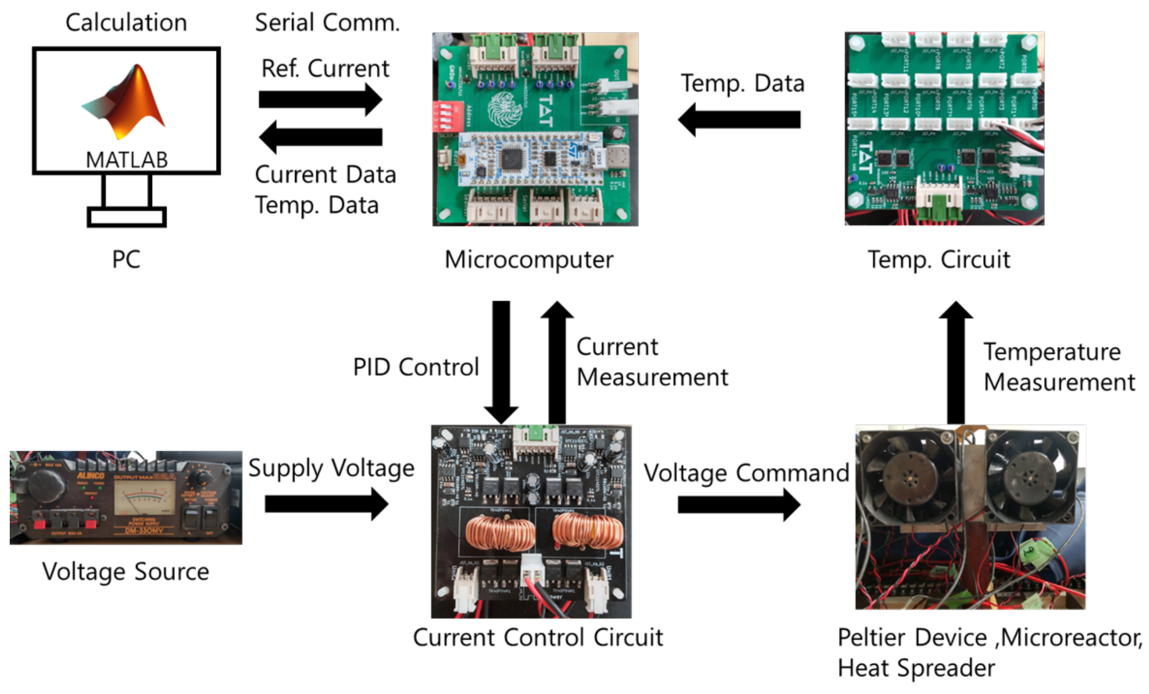
4.1. Experimental System

Figure 5 shows a diagram of the experimental apparatus. The experimental apparatus consists of a computer, power supply, microcomputer, temperature sensor circuit, current sensor circuit, and microreactor cooling block. The cooling block consists of a Peltier element, a heat spreader, a microreactor, and a fan. The microreactor and heat spreader are equipped with multiple temperature sensors. The operation flow of the system is shown below.
  • Temperature acquisition
    When the computer sends a command to the microcomputer to acquire the temperature, the microcomputer acquires the value from the temperature sensor circuit and sends the temperature value to the computer.
  • Control input calculation and current value setting
    Control inputs are calculated from operator theory based on target and acquisition temperatures. If necessary, the control input is converted to a current value. The calculated current value is sent to the microcomputer as a command current.
  • Current control
    The microcomputer performs PID control so that the current flowing through the Peltier element becomes the command current value received from the computer.
  • Step 1 is repeated until the control time is reached.
Table 7 shows the common parameters used in the simulations and the actual experiments. A first-order low-pass filter with a cutoff frequency of 10 Hz was used for noise rejection in the actual experiment.

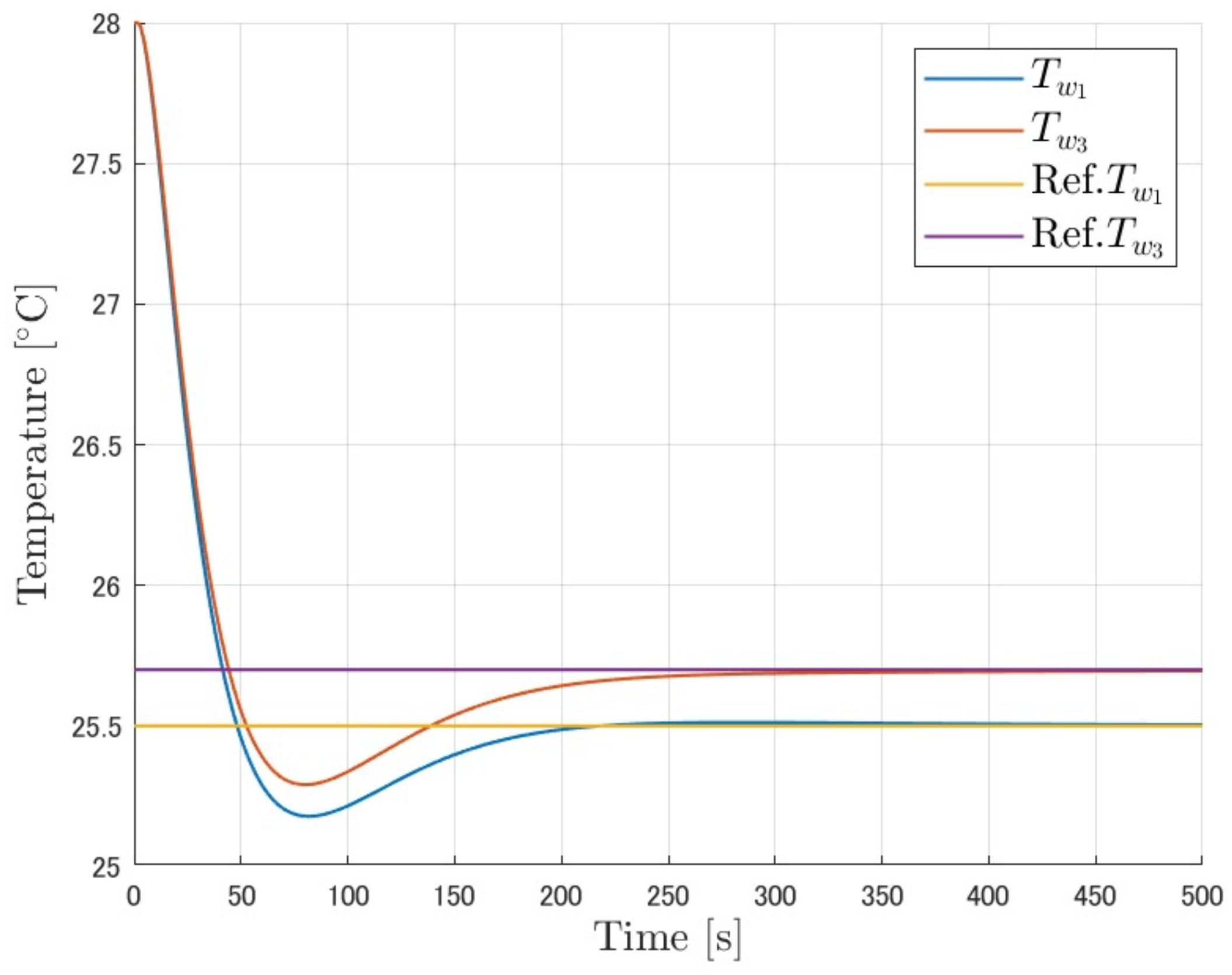
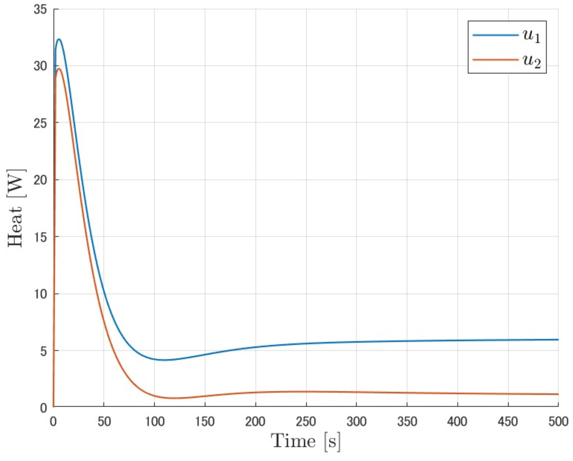
4.2. Simulation Results for MIMO Control Systems

Figure 6 and Figure 7 show the simulation results for the MIMO control system. The parameters used in the simulations are listed in Table 8. Figure 6 shows that T w 1 and T w 3 follow each other in about 150 s.

4.3. Results of Experiment

4.3.1. MIMO Control System

The experimental results of the MIMO control system are shown in Figure 8 and Figure 9. Table 9 shows the parameters used in the experiments. Figure 8 shows that T w 1 and T w 3 follow each other in about 250 s.

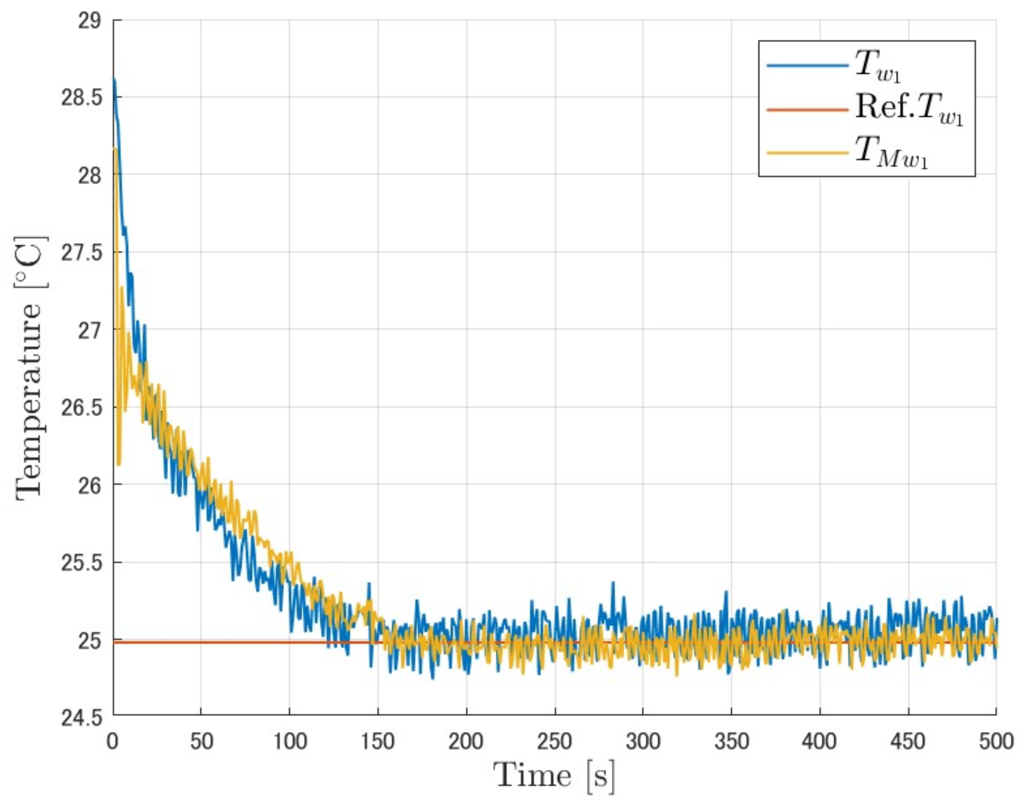
4.3.2. MIMO Sensorless Control Using M–SVR

Figure 10, Figure 11 and Figure 12 show the experimental results of sensorless control using M–SVR. Table 10 shows the parameters used in the experiments. Here, T M w 1 and T M w 3 are the estimated values of M–SVR and are the signals used for feedback, while T w 1 and T w 3 are only measurements and are not used for control. Figure 10 and Figure 11 show that the estimated values of T M w 1 and T M w 3 of M–SVR follow each other in about 320 s.

4.4. Discussion

Compare Figure 6 and Figure 7, which are simulation results of the control system in Figure 3, Figure 8 and Figure 9, which are the results of actual machine experiments. Figure 9, which is a graph of temperature, shows an overshoot, whereas Figure 8 does not. In addition, the simulation results show a faster target value tracking time than the experimental results. This is due to the fact that the heat spreader used in the experimental system has a cavity, which has a smaller thermal conductivity than in reality. And, even though the difference between the two cooling temperatures is larger in the actual experiment than in the simulation, the simulation results are more biased than Figure 7 and Figure 9. The reason for this is that the heat spreader used in the experimental system has a cavity, which is not taken into account, and therefore the thermal conductivity of the model is larger than in reality. From Figure 10 and Figure 11, which are the results of the sensorless control system using M–SVR, it can be seen that there are errors between the sensor values and the estimated values. This is due to modeling errors that occur when the model is created via M–SVR.

5. Conclusions

In this study, a MIMO temperature control system for a microreactor was designed and its effectiveness was confirmed through simulations and experiments. The proposed method can control two temperatures in a microreactor, whereas the conventional method can control only one temperature in a microreactor, thus allowing for a high degree of freedom in temperature control. We also created a machine learning model of the M–SVR of a microreactor using a generalized Gaussian kernel and conducted actual experiments on sensorless control using the model to confirm its effectiveness. The hyperparameters of the M–SVR were optimized using a real-coded genetic algorithm, one of the metaheuristics, and then adjusted manually. The MSE of each output was lower for the generalized Gaussian kernel than for the RBF kernel, indicating the accuracy of the model. In addition, the fact that the M–SVR estimates from the experiment are distributed near the corresponding sensor values confirms that they are correctly estimated and confirms the effectiveness of sensorless control.

Author Contributions

T.K. applied a generalized Gaussian kernel as the kernel function of M–SVR and performed parameter optimization using a real-coded genetic algorithm. Using the model, a sensorless control of a MIMO temperature control system of a microreactor was proposed. In addition, K.N. proposed a method to extend the temperature control system of a microreactor to a MIMO temperature control system, and M.D. suggested technical support and gave overall guidance on the paper. All authors have read and agreed to the published version of the manuscript.

Funding

This research received no external funding.

Institutional Review Board Statement

Not applicable.

Informed Consent Statement

Not applicable.

Data Availability Statement

Data are contained within the article.

Conflicts of Interest

The authors declare no conflicts of interest.

Abbreviations

The following abbreviations are used in this manuscript:
MIMOMulti-input multi-output
M–SVRMulti-output support vector regression
MSEMean square error

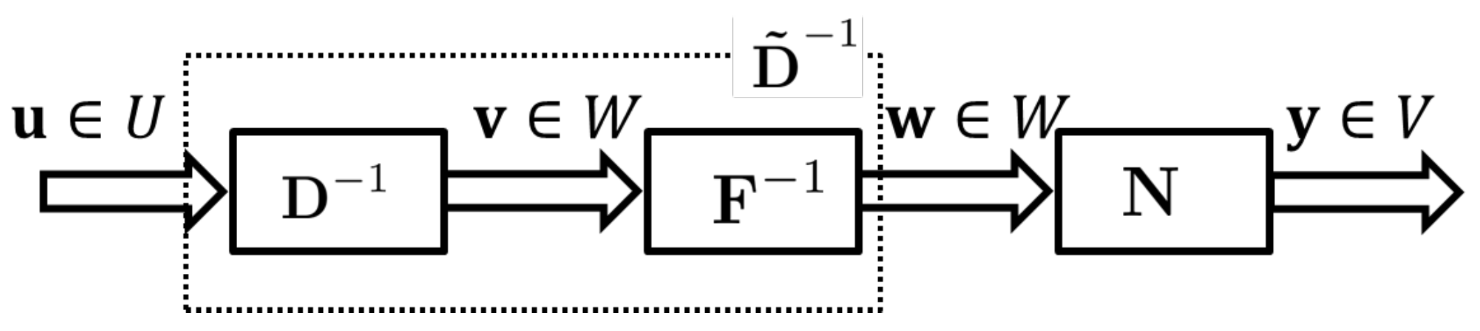
Appendix A. Separation of Coupling Elements

When performing MIMO temperature control, it is necessary to consider the coupling elements that occur between each control system. In this study, the coupling elements are separated based on Reference [8], and the two-input, two-output control system is divided into two independent subsystems for control. Figure A1 shows a MIMO system plant with coupling elements. Here, U is the input space, V is the output space, and u = ( u 1 , u 2 , , u n ) , y = ( y 1 , y 2 , , y n ) are the inputs and outputs of the nominal plant P = ( P 1 , P 2 , , P n ) : U V. The operator N = ( N 1 , N 2 , , N n ) : W V is nonlinear and stable, and P is diagonalizable. The plant can then undergo right factorization as follows.
P = N D ˜ 1
where D is linear, stable and invertible. We define the operator F with respect to the coupling elements, as in the following equation, where f is a bounded unknown.
v ( t ) = F ( w ) ( t ) = F · w ( t ) + f ( t ) w = ( w 1 , w 2 , w n ) W v = ( v 1 , v 2 , v n ) W f = ( f 1 , f 2 , f n ) W
In this case, D ˜ can be expressed as follows:
D ˜ = DF : W U
Next, consider a MIMO system with feedback signals as shown in Figure A2, where S is the feedback operator and b is the feedback signal b = S ( y ) .
Figure A1. MIMO system plant.
Computation 12 00002 g0a1
Figure A2. MIMO system stabilization via operator theory.
Computation 12 00002 g0a2
Each element b i of the feedback signal b is expressed by the following equation, which includes the coupling elements.
b i = j = i n S i j ( y i )
However, the coupling factor can be eliminated by designing the operator to satisfy the following equation.
S i j N j + F i j D i = 0 , j i R i , j = i
In this case, the coupling factor is removed from the input u as in the following equation, which can be converted to an equation including the disturbances f and ω .
u i ( t ) = D i ( v i ) + j = i n S i j ( y i ) ( t )
= D i ( f i ) + j = i n ( S i j N j + D i F i j ) ( ω j ) ( t )
= D i ( f i ) + R i ( ω i ) ( t )
The right factorization can then be transformed as follows.
P ˜ i = N i R i 1

Appendix B. M–SVR

M–SVR (Multi-output Support Vector Regression) is an SVR for multi-output problems and is a regression analysis method that can take into account the effects among outputs [28,29]. Consider the case of d input ( x R d ) and Q output ( y R Q ). Assuming j = 1 , 2 , , Q , the jth coefficient vector is w j R d and the bias is b j R , the regression equation f becomes Equation (A10).
f j ( x ) = ( w j ) x + b j
Let f ( x ) = [ f 1 ( x ) , f 2 ( x ) , , f Q ( x ) ] R Q , W = [ w 1 , w 2 , , w Q ] R d × Q , b = [ b 1 , b 2 , , b Q ] R Q , and ϕ ( x ) be a function ϕ ( x ) : R d F that maps the input x to the feature space F. The regression equation for M–SVR is Equation (A11).
f ( x ) = W ϕ ( x ) + b
Let e i = y i f ( x i ) and u i = e i = e i e i , and define the cost function L p ( W , b ) and the loss function L ( u ) as Equations (A12) and (A13).
L p ( W , b ) = 1 2 j = 1 Q w j 2 + C i = 1 l L ( u i )
L ( u ) = 0 u < ϵ u 2 2 u ϵ + ϵ 2 u ϵ
C is the regularization factor and ϵ is the insensitivity parameter. The M–SVR used in this study determines the parameters of the optimal regression equation using a type of iterative method called IRWLS (Iterative Reweighted Least Square). To construct IRWLS, Equation (A12) is first-order Taylor-expanded.
L P ( W , b ) = 1 2 j = 1 Q w j 2 +   C i = 1 n L ( u i k ) + d L ( u ) d u | u i k ( e i k ) u i k [ e i e i k ]
where u i k = e i k = e i k e i k , e i k = y i ϕ x i W k b k .
This is the quadratic approximation of Equation (A14).
L P ( W , b ) = 1 2 j = 1 Q w j 2
+   C i = 1 n L ( u i k ) + d L ( u ) d u | u i k u i 2 u i k 2 2 u i k
= 1 2 j = 1 Q w j 2 + 1 2 i = 1 n a i u i 2 + C T
a i can be expressed as in Equation (A17).
a i = C u i k d L ( u ) d u | u i k = 0 u i k < ϵ 2 C u i k ϵ u i k u i k ϵ
In addition, C T is a term that represents the sum of constants and does not depend on W or b . The IRWLS algorithm is shown below.
  • Initialize k = 0 , W k = 0 , b k = 0 , and compute u i k and a i .
  • Equation (A15) is calculated and the obtained W and b are defined as W s and b s . The decreasing direction P in Equation (A12) is defined as Equation (A18).
    P = W s W k b s b k
  • The solution of the next step is obtained from Equation (3). η k is calculated via a backtracking algorithm.
    W k + 1 b k + 1 = W k b k + η k P k
  • Compute u i k , a i .Return to 2 until convergence.
In the following, we will address how to obtain W s and b s . To obtain W s and b s , it is necessary to solve the weighted least-squares problem in Equation (A16). Then, by partial differentiation of Equation (A16) with w j and b j , and setting their slopes to zero, Equations (A20) and (A21) are obtained.
w j L P = w j i ϕ x i a i y i j ϕ x i w j b j = 0
b j L P = i a i y i j ϕ x i w j b j = 0
where 0 R d . Equations (A20) and (A21) can be expressed in matrix notation as in Equation (A22).
Φ D a Φ + I Φ a a Φ 1 a w j b j = Φ D a y j a y j
where Φ = ϕ x 1 , , ϕ x n R d × n , a = a 1 , , a n R n , y j = y 1 j , , y n j R n , D = d i a g a R n × n and 1 R n .
Next, a feature space kernel is introduced to accommodate nonlinearities. Substituting the Representer Theorem w j = i ϕ x i β j = Φ β j into Equations (A20) and (A21), we obtain Equation (A23).
K + D a 1 1 a K 1 a β j b j = y j a y j
where K i j = κ x i , x j . By changing W s β s to W k β k and W k to β k in the IRWLS algorithm described earlier, nonlinear multiple-output support vector regression can be realized.

Appendix C. Generalized Gaussian Kernel

The generalized Gaussian kernel is a kernel based on a generalized Gaussian distribution [27]. Equation (A24) shows the generalized Gaussian function.
f ( x ) = g γ γ 2 σ Γ 1 / γ exp g γ x μ e σ γ
g γ = Γ 3 / γ Γ 1 / γ
x R n is the input, μ is the mean, σ is the standard deviation, γ is the shape parameter, e R n is the unit vector, and Γ z is the gamma function. The shape parameter is also called the decay ratio because a smaller value of the shape parameter γ results in a sharper probability density function, while a larger value results in a flatter probability density function.
Based on the above, the generalized Gaussian kernel is shown in Equation (A26).
f x i , x j = g γ γ 2 σ Γ 1 / γ exp g γ x i x j σ γ

References

  1. Hinterleitner, B.; Knapp, I.; Poneder, M.; Shi, Y.; Müller, H.; Eguchi, G.; Eisenmenger-Sittner, C.; Stöger-Pollach, M.; Kakefuda, Y.; Kawamoto, N.; et al. Thermoelectric performance of a metastable thin-film Heusler alloy. Nature 2019, 576, 85–90. [Google Scholar] [CrossRef] [PubMed]
  2. Zhao, D.; Tan, G. A review of thermoelectric cooling: Materials, modeling and applications. Appl. Therm. Eng. 2014, 66, 15–24. [Google Scholar] [CrossRef]
  3. Deng, M.; Iwai, Z.; Mizumoto, I. Robust parallel compensator design for output feedback stabilization of plants with structured uncertainty. Syst. Control Lett. 1999, 36, 193–198. [Google Scholar] [CrossRef]
  4. Rsetam, K.; Cao, Z.; Man, Z. Design of Robust Terminal Sliding Mode Control for Underactuated Flexible Joint Robot. IEEE Trans. Syst. Man Cybern. Syst. 2022, 52, 4272–4285. [Google Scholar] [CrossRef]
  5. Man, Z.; Paplinski, A.P.; Wu, H. A robust MIMO terminal sliding mode control for rigid robotic manipulators. IEEE Trans. Autom. Control 1994, 39, 2264–2469. [Google Scholar]
  6. Wang, H.; Man, Z.; Kong, H.; Zhao, Y.; Yu, M.; Cao, Z.; Zheng, J.; Do, M.T. Design and Implementation of Adaptive Terminal Sliding-Mode Control on a Steer-by-Wire Equipped Road Vehicle. IEEE Trans. Ind. Electron. 2016, 63, 5774–5785. [Google Scholar] [CrossRef]
  7. Yu, X.; Man, Z. Model reference adaptive control systems with terminal sliding modes. Int. J. Control 1996, 64, 1165–1176. [Google Scholar] [CrossRef]
  8. Deng, M. Robust Stability of Operator-Based Nonlinear Control Systems. In Operator-Based Nonlinear Control Systems: Design and Applications; John Wiley & Sons, Ltd.: Hoboken, NJ, USA, 2014; pp. 27–115. [Google Scholar]
  9. Chen, G.; Han, Z. Robust right coprime factorization and robust stabilization of nonlinear feedback control systems. IEEE Trans. Autom. Control 1998, 43, 1505–1509. [Google Scholar] [CrossRef]
  10. Deng, M.; Inoue, A.; Goto, S. Operator based Thermal Control of an Aluminum Plate with a Peltier Device. Int. J. Innov. Comput. Inf. Control 2008, 4, 3219–3229. [Google Scholar]
  11. Matsui, A.; Meng, L.; Hattori, K. Enhanced YOLO using Attention for Apple grading. In Proceedings of the 2023 International Conference on Advanced Mechatronic Systems (ICAMechS), Melbourne, Australia, 4–7 September 2023. [Google Scholar]
  12. Li, Z.; Meng, L. Research on Deep Learning-based Cross-disciplinary Applications. In Proceedings of the 2022 International Conference on Advanced Mechatronic Systems (ICAMechS), Toyama, Japan, 17–20 December 2022. [Google Scholar]
  13. Atsumi, M.; Kawano, S.; Morioka, T.; Meng, L. Deep Learning Based Ancient Asian Character Recognition. In Proceedings of the 2020 International Conference on Advanced Mechatronic Systems (ICAMechS), Hanoi, Vietnam, 10–13 December 2020. [Google Scholar]
  14. Zhang, Y.; Meng, L.; Xue, X.; Zhou, Z.; Tomiyama, H. QoE-Constrained Concurrent Request Optimization through Collaboration of Edge Servers. IEEE Internet Things J. 2019, 6, 9951–9962. [Google Scholar] [CrossRef]
  15. Meng, L.; Hirayama, T.; Oyanagi, S. Underwater-Drone with Panoramic Camera for Automatic Fish Recognition Based on Deep Learning. IEEE Access 2018, 6, 17880–17886. [Google Scholar] [CrossRef]
  16. Chen, L.; Li, X.; Ma, L.; Bi, S. Probabilistic neural network based apple classification prediction. In Proceedings of the 2022 International Conference on Advanced Mechatronic Systems (ICAMechS), Toyama, Japan, 17–20 December 2022. [Google Scholar]
  17. Bi, S.; Qu, X.; Ma, L.; Shen, T.; Han, C. Apple Grading Method Based on Ordered Partition Neural Network. In Proceedings of the 2021 International Conference on Advanced Mechatronic Systems (ICAMechS), Tokyo, Japan, 9–12 December 2021. [Google Scholar]
  18. Wang, C.; Man, Z.; Jin, J.; Ye, W. Hash-Based Convolutional Deep-thinking Pattern Classifier. In Proceedings of the 2023 International Conference on Advanced Mechatronic Systems (ICAMechS), Melbourne, Australia, 4–7 September 2023. [Google Scholar]
  19. Gao, X.; Yang, Q.; Zhang, J. Multi-objective optimisation for operator-based robust nonlinear control design for wireless power transfer systems. Int. J. Adv. Mechatron. Syst. 2022, 9, 203–210. [Google Scholar] [CrossRef]
  20. Zhang, Z.; Wen, F.; Shi, J.; He, J.; Truong, T.-K. 2D-DOA Estimation for Coherent Signals via a Polarized Uniform Rectangular Array. IEEE Signal Process. Lett. 2023, 30, 893–897. [Google Scholar] [CrossRef]
  21. Usami, T.; Deng, M. Applying an MSVR Method to Forecast a Three-Degree-of-Freedom Soft Actuator for a Nonlinear Position Control System: Simulation and Experiments. IEEE Syst. Man Cybern. Mag. 2022, 8, 61–69. [Google Scholar] [CrossRef]
  22. Bu, N.; Zhang, Y.; Li, X. Robust tracking control for uncertain micro-hand actuator with Prandtl-Ishlinskii hysteresis. Int. J. Robust Nonlinear Control 2023, 33, 9391–9405. [Google Scholar] [CrossRef]
  23. Bu, N.; Liu, H.; Li, W. Robust passive tracking control for an uncertain soft actuator using robust right coprime factorization. Int. J. Robust Nonlinear Control 2021, 31, 6810–6825. [Google Scholar] [CrossRef]
  24. Bu, N.; Wang, X. Swing–up design of double inverted pendulum by using passive control method based on operator theory. Int. J. Adv. Mechatron. Syst. 2022, 1, 1. [Google Scholar] [CrossRef]
  25. An, Z.; Bu, N. Modeling for a Bellow-Shaped Soft Actuator Based on Yeoh model and Operator-Based Nonlinear Control Design. In Proceedings of the 2023 International Conference on Advanced Mechatronic Systems (ICAMechS), Melbourne, Australia, 4–7 September 2023. [Google Scholar]
  26. Deng, M.; Saijo, N.; Gomi, H.; Inoue, A. A robust real time method for estimating human multijoint arm viscoelasticity. Int. J. Innov. Comput. Inf. Control 2006, 2, 705–721. [Google Scholar]
  27. Deng, M.; Inoue, A.; Zhu, Q.M. An integrated study procedure on real-time estimation of time-varying multi-joint human arm viscoelasticity. Trans. Inst. Meas. Control 2011, 33, 919–941. [Google Scholar] [CrossRef]
  28. Sanchez-Fernandez, M.; de-Prado-Cumplido, M.; Arenas-Garcia, J.; Arenas-Garcia, F. SVM multiregression for nonlinear channel estimation in multiple-input multiple-output systems. IEEE Trans. Signal Process. 2004, 52, 2298–2307. [Google Scholar] [CrossRef]
  29. Tuia, D.; Verrelst, J.; Alonso, L.; Perez-Cruz, F.; Camps-Valls, G. Multioutput Support Vector Regression for Remote Sensing Biophysical Parameter Estimation. IEEE Geosci. Remote Sens. Lett. 2011, 8, 804–808. [Google Scholar] [CrossRef]
  30. Ono, I.; Kita, H.; Kobayashi, A. A Real-coded Genetic Algorithm using the Unimodal Normal Distribution Crossover. In Advances in Evolutionary Computing: Theory and Applications; Ghosh, A., Tsutsui, S., Eds.; Springer: Berlin/Heidelberg, Germany, 2003; pp. 213–237. [Google Scholar]
  31. Tsutsui, S.; Yamamura, M.; Higuchi, T. Multi-parent recombination with simplex crossover in real coded genetic algorithms. In Proceedings of the 1st Annual Conference on Genetic and Evolutionary Computation—Volume 1, Orlando, FL, USA, 13–17 July 1999. [Google Scholar]
Figure 1. Model of microreactor and heat spreader.
Computation 12 00002 g001
Figure 2. Without interference effects.
Computation 12 00002 g002
Figure 3. MIMO control system for microreactor based on operator theory.
Computation 12 00002 g003
Figure 4. Proposed sensorless control system using M–SVR.
Computation 12 00002 g004
Figure 5. Diagram of the experimental apparatus.
Computation 12 00002 g005
Figure 6. Microreactor temperature (simulation on MIMO control system).
Computation 12 00002 g006
Figure 7. Control input (simulation on MIMO control system).
Computation 12 00002 g007
Figure 8. Microreactor temperature (experiment on MIMO control system).
Computation 12 00002 g008
Figure 9. Control input (experiment on MIMO control system).
Computation 12 00002 g009
Figure 10. Microreactor temperature T w 1 and M–SVR estimate T M w 1 (experiment).
Computation 12 00002 g010
Figure 11. Microreactor temperature T w 3 and M–SVR estimate T M w 3 (experiment).
Computation 12 00002 g011
Figure 12. Control input (experiment on MIMO sensorless control using M–SVR).
Computation 12 00002 g012
Table 1. Parameters of area.
SymbolValueUnitSymbolValueUnit
S 1 2.6 × 10 3 m 2 S 2 7.0 × 10 4 m 2
S 3 9.8 × 10 3 m 2 S 4 9.0 × 10 4 m 2
S 5 9.0 π × 10 6 m 2 S 6 3.0 π × 10 4 m 2
S 7 1.4 × 10 3 m 2 S 8 2.8 × 10 4 m 2
S 9 1.2 π × 10 4 m 2
Table 2. Parameters of microreactor.
SymbolDescriptionValueUnit
T 0 Initial temperature-[ K ]
T a n Aluminum temperature ( n = 1 , 2 , 3 ) -[ K ]
T w k Water temperature ( k = 1 , 2 , 3 ) -[ K ]
y a n Aluminum cooling
temperature
-[ K ]
y w k Water cooling temperature-[ K ]
u d 1 , u d 2 Heat absorption from Peltier element-[ W ]
c a Specific heat of aluminum468 J / ( k g · K )
c w Specific heat of water2174.64 J / ( k g · K )
λ a Thermal conductivity of aluminum238 J / ( k g · K )
λ w Thermal conductivity of water0.602 J / ( k g · K )
α Heat transfer
coefficient of air
180 W / ( m 2 · K 4 )
α w Heat transfer
coefficient of water
500 W / ( m 2 · K 4 )
m a 1 , m a 3 Mass of HS1.31 k g
m a 2 Mass of HS0.52 k g
m w 1 , m w 3 Mass of Water 1.41 × 10 3 k g
m w 2 Mass of Water 0.6 × 10 3 k g
σ Stefan–Boltzmann constant 5.67 × 10 8 W / ( m 2 · K 4 )
ϵ a Thermal emissivity of aluminum0.2-
ϵ w Thermal emissivity of water0.93-
Table 3. Parameters of RBF.
SymbolDescriptionValue
CRegularization parameter 106.8
ϵ Insensitive factor 0.0077
γ Kernel coefficient for RBF 0.371
Table 4. Parameters of generalized Gaussian kernel.
SymbolDescriptionValue
CRegularization parameter 251.96
ϵ Insensitive factor 6.32 × 10 4
γ Shape parameter 0.5151
σ Standard deviation 48.007
Table 5. MSE comparison.
Description PartW 1 PartW 2 PartW 3 PartA 1 PartA 3
RBF 0.0020 0.0015 0.0015 0.0016 0.0015
GGD 0.0015 0.0010 0.0011 0.0011 0.0011
Table 6. Parameters of Peltier device.
SymbolDescriptionValueUnit
SSeebeck coefficient0.08 V / K
RElectrical resistance2 Ω
KThermal conductance0.43 W / K
Table 7. Common parameters for simulation and experiment.
SymbolDescriptionValueUnit
T s Control time500 s
t Control cycle1 s
B w 1 , B w 3 Design parameter0.999
n a 1 , n a 3 Design parameter1000
n w 1 , n w 3 Design parameter1000
Table 8. Parameters for simulation.
SymbolDescriptionValueUnit
T 0 Initial temperature28 C
r 1 Reference of Part W 1 2.5 C
r 2 Reference of Part W 3 2.3 C
k p 1 , k p 3 Proportional gain of Part W 1 , W 3 0.02
k i 1 , k i 3 Integral gain of Part W 1 , W 3 0.00032
Table 9. Parameters of experiment on MIMO control systems.
SymbolDescriptionValueUnit
T 0 Initial temperature 21.69 C
r 1 Reference of Part W 1 2.0 C
r 2 Reference of Part W 3 2.5 C
k p 1 , k p 3 Proportional gain of Part W 1 , W 3 0.001
k i 1 , k i 3 Integral gain of Part W 1 , W 3 0.0002
Table 10. Parameters of experiment on MIMO sensorless control using M–SVR.
SymbolDescriptionValueUnit
T 0 Initial temperature 27.68 C
r 1 Reference of Part W 1 2.7 C
r 2 Reference of Part W 3 2.5 C
k p 1 , k p 3 Proportional gain of Part W 1 , W 3 0.001
k i 1 , k i 3 Integral gain of Part W 1 , W 3 0.0002
Disclaimer/Publisher’s Note: The statements, opinions and data contained in all publications are solely those of the individual author(s) and contributor(s) and not of MDPI and/or the editor(s). MDPI and/or the editor(s) disclaim responsibility for any injury to people or property resulting from any ideas, methods, instructions or products referred to in the content.

