1. Introduction
Machine learning (ML) has numerous applications in modeling and simulation of structures [
1]. One of the most common applications of ML in structural analysis is the prediction of structural behavior under different loads and environmental conditions. ML algorithms can be trained on data from previous structural analyses, to learn how different factors—such as material properties, geometry, and loading conditions—affect structural response. This information can then be used to predict the behavior of new structures, without the need for time-consuming and expensive additional analyses. Another interesting field of application is structural health monitoring (SHM) and damage identification [
2], where, by analyzing the changes in structural response over time, and using data collected by SHM systems, ML algorithms can learn to detect and localize damage in structures and, in general, assess the health and condition of a structure over time. In design optimization [
3], by analyzing the relationships between different design parameters and structural performance, ML algorithms can identify optimal design configurations that minimize weight, maximize stiffness, or achieve other desired performance characteristics [
4,
5]. ML can be also used to quantify the uncertainties associated with structural analyses, improving the accuracy of predictions and reducing the risk of failure [
6]. Overall, the use of ML in structural analysis has the potential to significantly improve the accuracy and efficiency of structural analysis, as well as to enable new capabilities for damage detection and design optimization.
In the specialized fields of structural dynamics and earthquake engineering, ML techniques are also increasingly being used [
7], as they can help to extract useful insights and patterns from large amounts of data, which can be used to improve the accuracy and efficiency of structural dynamic analysis techniques. Data-driven models for predicting the dynamic response of linear and non-linear systems are of great importance, due to their wide application, from probabilistic analysis to inverse problems, such as system identification and damage diagnosis. In the following paragraphs, we examine some important works and state-of-the-art contributions in the field.
Xie et al. [
8] presented a comprehensive evaluation of the progress and challenges of implementing ML in earthquake engineering. Their study used a hierarchical attribute matrix to categorize the literature, based on four traits, (i) ML method; (ii) topic area; (iii) data resource; and (iv) scale of analysis. Their review examined the extent to which ML has been applied in several areas of earthquake engineering, including structural control for earthquake mitigation, seismic fragility assessment, system identification and damage detection, and seismic hazard analysis. Zhang et al. [
9] presented a ML framework to assess post-earthquake structural safety. They proposed a systematic methodology for generating a reliable dataset for any damaged building, which included the incorporation of the concepts of response and damage patterns. The residual collapse capacity of the damaged structure was evaluated, using incremental dynamic analysis with sequential ground motions. ML algorithms were employed, to map response and damage patterns to the safety state of the building, based on a pre-determined threshold of residual collapse capacity.
Nguyen et al. [
10] applied ML techniques to predict the seismic responses of 2D steel moment-resisting frames under earthquake motions. They used two popular ML algorithms—Artificial Neural Network (ANN) and eXtreme Gradient Boosting (XGBoost)—and took into consideration more than 22,000 non-linear dynamic analyses, on 36 steel moment frames of various structural characteristics, under 624 earthquake records with peak accelerations greater than 0.2 g. Both ML algorithms were able to reliably estimate the seismic drift responses of the structures, while XGBoost showed the best performance. Sadeghi Eshkevari et al. [
11] proposed a physics-based recurrent ANN that was capable of estimating the dynamic response of linear and non-linear multiple degrees of freedom systems, given the ground motions. The model could estimate a broad set of responses, such as acceleration, velocity, displacement, and the internal forces of the system. The architecture of the recurrent block was inspired by differential equation solver algorithms. The study demonstrated that the network could effectively capture various non-linear behaviors of dynamic systems with a high level of accuracy, without requiring prior information or excessively large datasets.
In the interesting work of Abd-Elhamed et al. [
12], logical analysis of data (LAD) was employed to predict the seismic responses of structures. The authors used real ground motions, considering a variation of earthquake characteristics, such as soil class, characteristic period, time step of records, peak ground displacement, peak ground velocity, and peak ground acceleration. The LAD model was compared to an ANN model, and was proven to be an efficient tool with which to learn, simulate, and predict the dynamic responses of structures under earthquake loading. Gharehbaghi et al. [
13] used multi-gene genetic programming (MGGP) and ANNs to predict seismic damage spectra. They employed an inelastic SDOF system under a set of earthquake ground motion records, to compute exact spectral damage, using the Park–Ang damage index. The ANN model exhibited better overall performance, yet the MGGP-based mathematical model was also useful, as it managed to provide closed mathematical expressions for quantifying the potential seismic damage of structures.
Kazemi et al. [
14] proposed a prediction model for seismic response and performance assessment of RC moment-resisting frames. They conducted incremental dynamic analyses (IDAs) of 165 RC frames with 2 to 12 stories and bay length ranging from 5.0 m to 7.6 m, ending up with a total of 92,400 data points for training the developed data-driven models. The examined output parameters were the maximum interstory drift ratio and the median of the IDA curves, which can be used to estimate the seismic limit state capacity and performance assessment of RC buildings. The methodology was tested in a five-story RC building with very good results. Kazemi and Jankowski [
15] used supervised ML algorithms in Python, to find median IDA curves for predicting the seismic limit-state capacities of steel moment-resisting frames considering soil–structure interaction effects. They used steel structures of two to nine stories subjected to three ground motion subsets as suggested by FEMA-P695, and 128,000 data points in total. They developed a user-friendly graphical user interface (GUI) to predict the spectral acceleration
of seismic limit-state performance levels using the developed prediction models. The developed GUI mitigates the need for computationally expensive, time-consuming, and complex analysis, while providing the median IDA curve including soil–structure interaction effects.
Wakjira et al. [
16] presented a novel explainable ML-based predictive model for the lateral cyclic response of post-tensioned base rocking steel bridge piers. The authors implemented a wide variety of nine different ML techniques, ranging from the simple to most advanced ones, to generate the predictive models. The obtained results showed that the simplest models were inadequate to capture the relationship between the input factors and the response variables, while advanced models, such as the optimized XGBoost, exhibited the best performance with the lowest error. Simplified and approximate methods are particularly useful in engineering practice and have been successfully used by various researchers in structural dynamics and earthquake engineering related applications, such us the evaluation of the seismic performance of steel frames [
17] and others.
The novelty of the present work consists of the development of new optimized ML models for the accurate and computationally efficient predictions of the fundamental eigenperiod, the maximum displacement as well as the base shear force of multi-story shear buildings. Four different ML algorithms are compared in terms of their prediction performance. The interpretation and explanation are elaborated using the permutations explainers of the SHAP methodology. In addition, a web application is developed based on the optimized ML models, to be easily used by engineers in practice. The remainder of the paper is organized as follows.
Section 2 defines the problem formulation, followed by the description of the dataset and the exploratory data analysis in
Section 3.
Section 4 provides an overview of ML algorithms, followed by the ML pipelines and performance results of
Section 5 and a discussion on interpretability of the results in
Section 6.
Section 7 presents and discussed the test case scenarios, while
Section 8 presents the web application that has been developed and deployed for broad and open use. In the end, a short discussion and the conclusions of the study are presented.
2. Problem Formulation
The response spectrum modal analysis (RSMA) is a method to estimate the structural response to short, non-deterministic, and transient dynamic events. Examples of such events are earthquakes and shocks. Since the exact time history of the load is not known, it is difficult to perform a time-dependent analysis. The method requires the calculation of the natural mode shapes and frequencies of a structure during free vibration. It uses the mass and stiffness matrices of a structure to find the various periods at which it will naturally resonate, and it is based on mode superposition, i.e., a superposition of the responses of the structure for its various modes, and the use of a response spectrum. The idea is to provide an input that gives a limit to how much an eigenmode having a certain natural frequency and damping can be excited by an event of this type. The response spectrum is used to compute the maximum response in each mode, instead of solving the time history problem explicitly using a direct integration method. These maxima are non-concurrent and for this reason the maximum modal responses for each mode cannot be added algebraically. Instead, they are combined using statistical techniques, such as the square root of the sum of the squares (SRSS) method or the more complex and detailed complete quadratic combination (CQC) method. Although the response spectrum method is approximate, it is broadly applied in structural dynamics and is the basis for the popular equivalent lateral force (ELF) method. In the following subsections, a brief description of the RSMA for multi-story structures is provided based on fundamental concepts of the single degree of freedom structural system.
2.1. Response Analysis of MDOF Systems
An idealized single degree of freedom (SDOF) shear building system has a mass
m located at its top and stiffness
k which is provided by a vertical column. For such a system without damping, the circular frequency
, the cyclic frequency
f and the natural period of vibration (or eigenperiod)
T are given by the following formulas:
Similar to the SDOF system, a multi-story shear building, idealized as a multi-degree of freedom (MDOF) system is depicted in
Figure 1, with the numbering of the stories from bottom to top. The vibrating system of the figure has
n stories and
n degrees of freedom (DOFs), denoted as the horizontal displacements
(
) at the top of each story. The dynamic equilibrium of a MDOF structure under earthquake excitation can be expressed with the following equation of motion at any time
t:
where
is the mass matrix of the structure holding the masses
at its diagonal;
is the stiffness matrix;
represents the damping matrix,
is the influence coefficient vector;
,
,
(all
) are the acceleration, velocity, and displacement vectors, respectively, and
is the ground motion acceleration, applied to the DOFs of the structure defined by the vector
.
The MDOF system has
n natural frequencies
(
) which can be found from the characteristic equation:
By solving the determinant of Equation (
3), one can find the eigenvalues
of mode
i which are the squares of the natural frequencies
of the system (
). Then, the eigenvectors (or mode shapes or eigenmodes
(each
n × 1) can be found by the following equation:
Equation (
4) represents a generalized eigenvalue problem, which is a classic problem in mathematics. The solution of this problem involves a series of matrix decompositions which can be computationally expensive, especially for large systems with many DOFs.
Let the displacement response of the MDOF system be expressed as
where
represents the modal displacement vector and
is the matrix containing the eigenvectors. Substituting Equation (
4) in Equation (
2) and pre-multiply by
we take
where
,
and
are the generalized mass, generalized damping, and generalized stiffness matrices, respectively. By virtue of the properties of the matrix
, the matrices
,
, and
are all diagonal matrices and Equation (
6) reduces to the following
where
is the modal displacement response of the
mode,
is the modal damping ratio of the
mode and
is the modal participation factor for the
mode, expressed by
where
is the
i-th element of the diagonal matrix
. Equation (
7) represents
n second order differential equations (i.e., similar to that of a SDOF system), the solution of which will provide the modal displacement response
for the
mode. Subsequently, the displacement response in each mode of the MDOF system can be obtained by Equation (
5) using the
.
2.2. Response Spectrum
In this work, we use the design spectrum for elastic analysis, as described in §3.2.2.5 of Eurocode 8 (EC8) [
18]. The inelastic behavior of the structure is taken into account indirectly by introducing the behavior factor
q. Based on this, an elastic analysis can be performed, with a response spectrum reduced with respect to the elastic one. The behavior factor
q is an approximation of the ratio of the seismic forces that the structure would experience if its response was completely elastic with 5% viscous damping, to the seismic forces that may be used in the design, with a conventional elastic analysis model, still ensuring a satisfactory response of the structure. For the horizontal components of the seismic action, the design spectrum,
, is defined as
where
T is the vibration period of a linear SDOF system,
S is the soil factor,
and
are the lower and upper limits of the period of the constant spectral acceleration branch, respectively,
is the value defining the beginning of the constant displacement response range of the spectrum,
is the design ground acceleration on type ‘A’ ground and
is the lower bound factor for the horizontal design spectrum, with a recommended value of 0.2. Although
q introduces a non-linearity into the system, for the sake of simplicity, in this study we assume elastic behavior of the structure by taking
q equal to 1. It has to be noted that we do not use the horizontal elastic response spectrum which is described in §3.2.2.2 of EC8, but rather the design spectrum for elastic analysis of §3.2.2.5, for the case
. The two are almost the same, but there are also some minor differences.
2.3. Response Spectrum Method for MDOF Systems
Given the spectrum, Equation (
7) is forming the equation of motion of a SDOF system. The maximum modal displacement response
is found from the response spectrum as follows:
Consequently, the maximum displacement (
) and acceleration (
) response of the MDOF system in the
mode are given as follows:
In each mode of vibration, the required response quantity of interest
Q, i.e., displacement, shear force, bending moment, etc., of the MDOF system can be obtained using the maximum response obtained by Equation (
11). However, the final maximum response
, is obtained by combining the response in each mode using a modal combination rule. In this study, the commonly square root of sum of squares (SRSS) rule is used as follows:
The SRSS method of combining maximum modal responses is fundamentally sound when the modal frequencies are well separated.
3. Dataset Description and Exploratory Data Analysis
The dataset was generated from 1995 results of dynamic response analyses of multi-story shear buildings of various configurations using the response spectrum method described in
Section 2. More specifically, the dataset consists of 3 features, namely (i) <Stories>, the number of stories in the shear building; (ii) <
>, the normalized stiffness over the mass of each story; and (iii) <Ground Type>, the ground type as the code provision (EC8) dictates. In addition, the dataset is completed with 3 targets, namely (i) <
>, the fundamental eigenperiod of the building; (ii) <
>, the horizontal displacement at the top story; and (iii) <
>, the normalized base shear force over the mass of each story of the building.
3.1. Dataset Description
In this study, we assume a constant k and m for all stories of the building, i.e., and remain constant for each story i. There is no change in the mass or stiffness of each story, along the height of the building. For such buildings, the response of the structure is characterized by the ratio rather than the individual values of k and m and this is the reason why , denoted as <> (normalized stiffness over mass), is taken as the input in the analysis, instead of taking into account the individual k and m for each story. The unit used for is (N/m)/kg which is equivalent to s. The normalized stiffness ranges from 2000 to 12,000 s (with a step of 500, i.e., 21 unique values), while the number of stories ranges from 2 to 20 (with a step of 1, resulting in 19 values), covering a wide range of the structures and representing the majority of typical multi-story shear buildings that can be found in practice.
The normalized base shear force over the mass of each story of the building has unit N/kg, which is equivalent to m·s. The ground acceleration for this study is kept constant at 1 g = 9.81 m/s as it affects the results in a linear way, since we assume elastic behavior (). As a result, all outputs are calculated with reference to an acceleration of 1 g. If another value is used for the ground acceleration, as is performed in the examined test scenarios, then the outputs of the model need to be multiplied with this ground acceleration value to obtain the correct results. A damping ratio of 5% was considered in all analyses.
All the targets, along with the input parameter <> are treated as continuous variables, while the remaining features are treated as integer variables. For the <Ground Type> feature, which natively takes values from the list of [‘A’, ‘B’, ‘C’, ‘D’, ‘E’], the ordinal encoding was used. In this encoding, each category value is assigned to an integer value due to the natural ordered relationship between each other, i.e., a type ‘B’ ground, is “worse” than a type ‘A’ ground, etc. Hence, the machine learning algorithms are able to understand and harness this relationship.
The final dataset, consists of 1995 observations in total, which is the product of 19 × 21 × 5, where 19 is the different numbers of stories, 21 are the different values of the normalized stiffness over the mass of each story, and 5 are the different ground types considered.
3.2. Exploratory Data Analysis
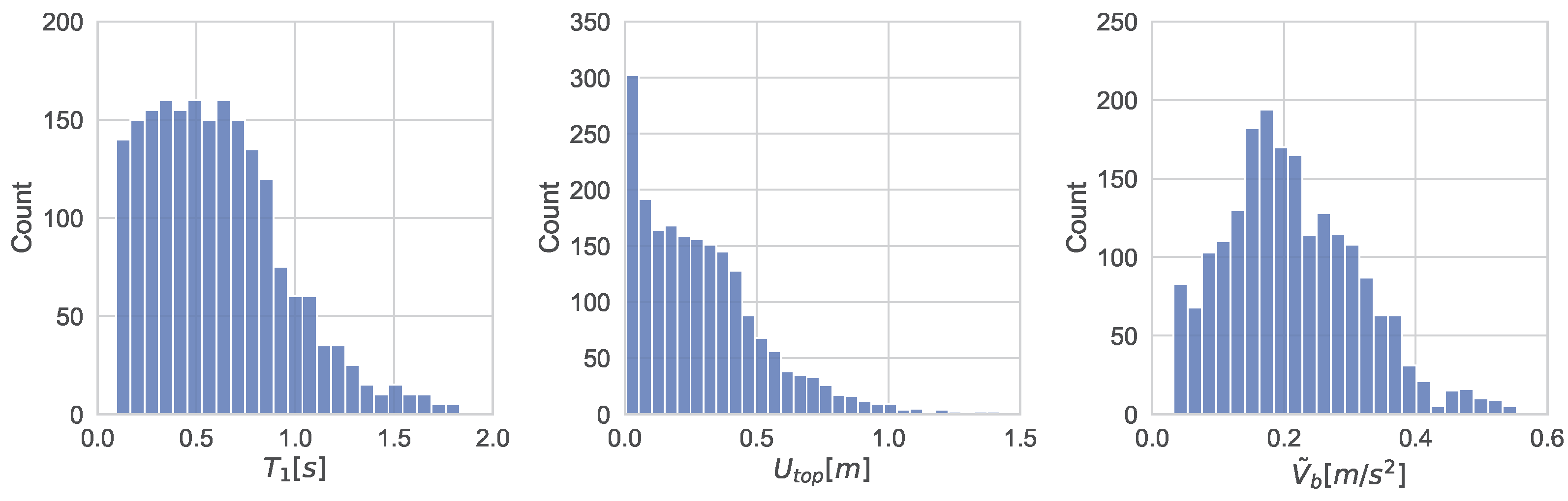
Understanding the data is very important before building any machine learning model. The statistical parameters and the distributions of dataset’s variables provide useful insights on the dataset and presented in
Table 1 and
Figure 2, respectively. From the latter one, it can be observed that all targets follow a right skewed unimodal distribution with platykurtic kurtosis (flatter than the normal distribution).
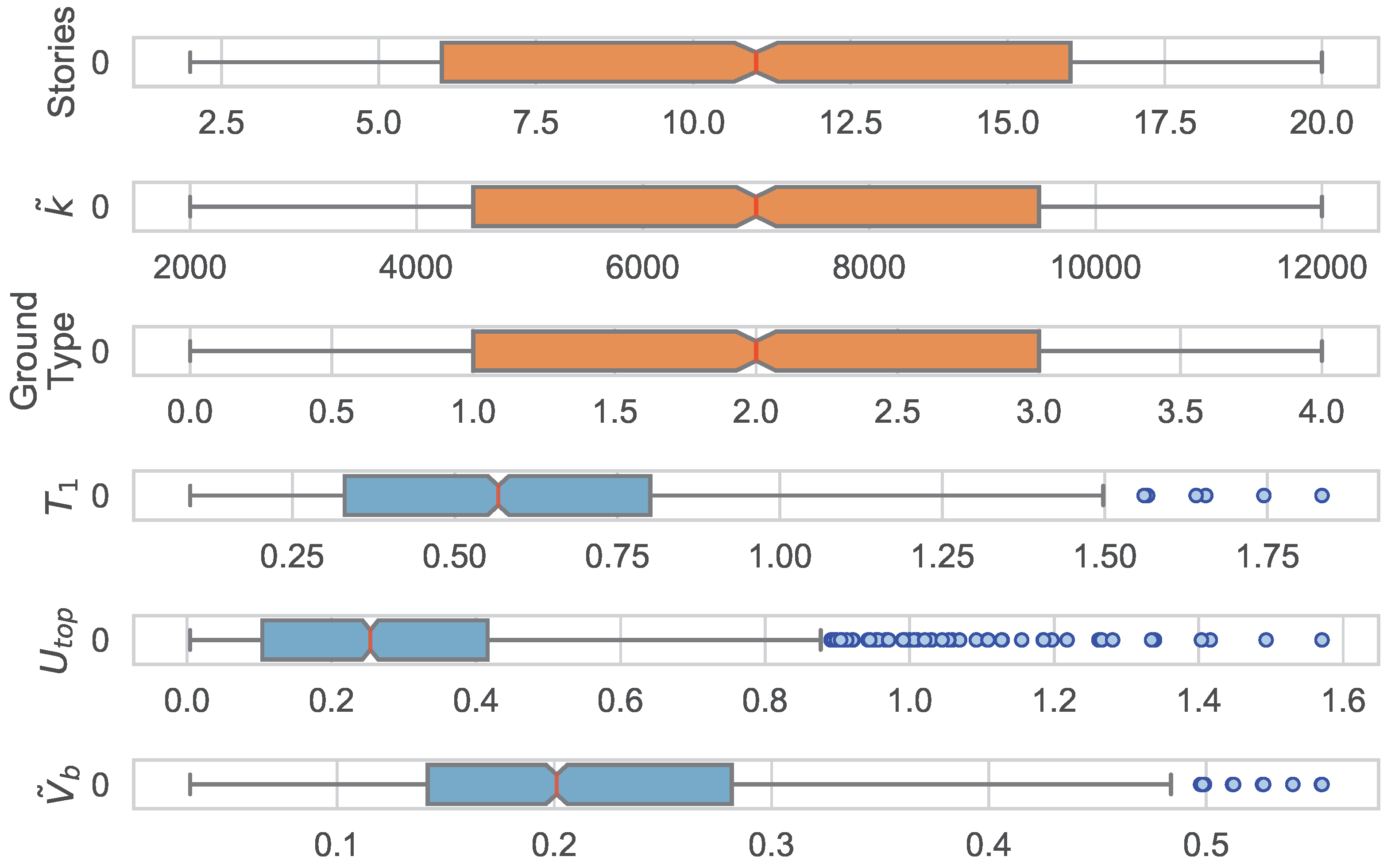
Figure 3 depicts the box and Whisker plots for features (orange) and targets (moonstone blue). The red vertical line shows the median of each distribution. The box shows the interquantile range (
) which measures the spread of the middle half of the data and contains 50% of the samples, defined as
, where
and
are the lower and upper quartiles, respectively. The black horizontal line shows the interval from the lower outlier gate
to the upper outlier gate
. As a result, the blue dots represent the “outliers” in each target, according to interquantile range (IQR) method. Often outliers are discarded because of their effect on the total distribution and statistical analysis of the dataset. However, in this situation, the occasional ’extreme’ building configurations (i.e., very flexible structures) cause an outlier that is outside the usual distribution of the dataset but is still a valid measurement.
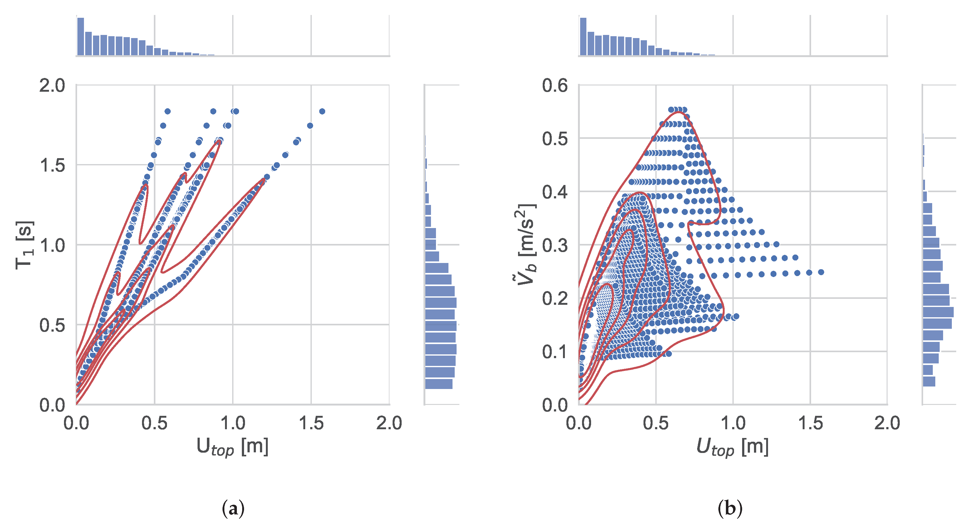
In
Figure 4, the joint plots with their kernel density estimate (KDE) plots for
feature against
and
are also depicted. KDE is a method for visualizing the distribution of observations in a dataset, analogous to a histogram and represents the data using a continuous probability density curve in two dimensions. Unlike a histogram, a KDE plot smooths the observations with a Gaussian kernel, producing a continuous density estimate. It can be observed that
and
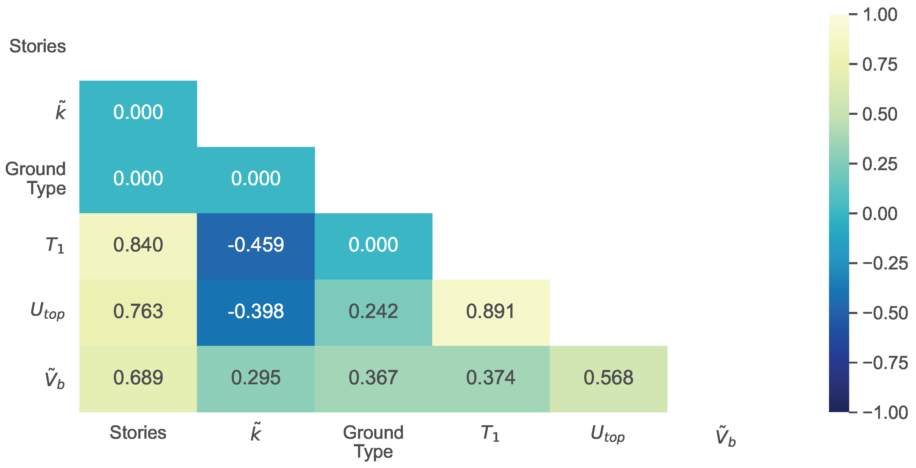
are correlated with a ‘linear’ type relation. This relation can be also derived from the high correlation values depicted in
Figure 5 that shows the correlation matrix of the dataset features and targets, including also the Pearson product-moment correlation coefficient. The Pearson product-moment correlation coefficient (
) is used to measure the correlation intensity between a pair of independent random variables (
x,
y), according to the following relation
where
is the covariance between the two random variables (
) and
,
is the standard deviation of x, y, respectively.
represents a
strong relationship between
x and
y, values between 0.3 and 0.8 represent
medium relationship, while
represents a
weak relationship. It is shown that the number of stories, has a strong relationship with
and
, while Ground Type has no relationship with the number of stories and
.
4. Overview of ML Algorithms
This study estimates the dynamic behavior of shear multi-story buildings in terms of predicting the fundamental eigenperiod (), the roof top displacement (), and the normalized base shear () by using four ML algorithms including Ridge Regressor (RR), Random Forest (RF) regressor, Gradient Boosting (GB), and Category Boosting (CB) regressor. All considered algorithms (except RR) belong to ensemble methods which seek better predictive performance by combining the predictions from multiple models usually in the form of decision trees by means of the bagging (bootstrap aggregating) and boosting ensemble learning techniques. Bagging involves fitting many decision trees (DTs) on different samples of the same dataset and averaging the predictions, while, in boosting, the ensemble members are added sequentially by correcting the predictions made by preceding models and the method outputs a weighted average of the predictions. Ensemble learning techniques eliminate any variance, thereby reducing the overfitting of models. In the following sections, an overview of each ML algorithm is provided, along with its strong and weak points.
4.1. Ridge Regression (RR)
With the absence of constraints, every model in machine learning will overfit the data and make unnecessary complex relationships. To avoid this, the regularization of data is needed. Regularization simplifies excessively complex models that are prone to be overfit and can be used to any machine learning model. Ridge regression [
19] is a regularized version of linear regression that uses the mean squared error loss function (LF) and applies L2 Regularization. In L2 Regularization (also known as Tikhonov Regularization), the penalty term is applied into the square of weights (
w) to the loss function as follows:
Consequently, the cost function
in Ridge Regression takes the following form
where
m is the total number of observations in the dataset,
n is the number of features in the dataset,
y and
are the ground truth and the predicted values of the regression model, respectively, and
is the penalty term which express the strength of regularization. The penalization in the sum of the squared weights reduces the variance of the estimates and the model, i.e., it shrinks the weights and, thus, reduces the standard errors. The penalty term serves to reduce the magnitude of the weights, and it also helps to prevent overfitting. As a result, RR can provide improved predictive accuracy and stability.
Ridge regression also has the ability to handle non-linear relationships between predictor and outcome variables, in contrast to linear regression. It is more robust to collinearity than linear regression and it can be applied to small datasets, while no perfect normalization of data is required. However, RR can be computationally expensive if the dataset is large. In addition, its results are difficult to interpret because the L2 regularization term modifies the weights. This is because the cost function contains a quadratic term, which makes it more difficult to optimize. In addition, RR only provides a closed-form approximation of the solution and can produce unstable results if outliers are present in the dataset.
Although, we a priori know that Ridge Regression will not able to compete with the other ensemble models, it is still selected as a simplistic method for a rough approximation of the model to be fitted.
4.2. Random Forest Regressor (RF)
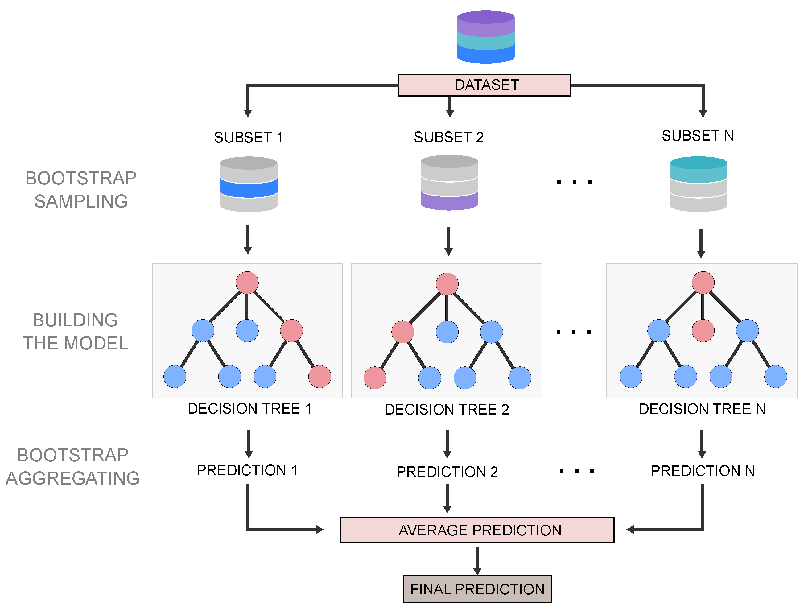
Decision trees are simple tree-like models of decisions that work well for many problems, but they can also be unstable and prone to overfitting. The Random Forest developed by Breiman [
20] overcomes these limitations by using an ensemble of decision trees as the weak learners, where each tree is trained on a random subset of the data and features (hence the name “Random Forest”). The subsets of the training data are created by random sampling with replacement (bootstrap sampling), thus, some data points may be included in multiple subsets, while others may not be included at all. Each model in the ensemble is trained independently using the same learning algorithm and hyperparameters, but with its own subset of the training data. The predictions from each tree are then combined by taking the average (
Figure 6). Therefore, this randomness helps reduce the variance of the model and the risk of overfitting problems in the decision tree method.
Random Forest is one of the most accurate machine learning algorithms which inherits the merits of the decision tree algorithm. It can work well with both categorical and continuous variables and can handle large datasets with thousands of features. Random Forest is a robust algorithm that can deal with noisy data and outliers and can generalize well to unseen data without the need of normalization as it uses a rule-based approach. Despite being a complex algorithm, it is fast and provides a measure of feature importance, which can help in feature selection and data understanding.
Although RF is less prone to overfitting than a single decision tree, it can still overfit the data if the number of trees in the forest is too high or if the trees are too deep. Random Forest can be less interpretable than a single decision tree because it involves multiple trees. Thus, it can be difficult to understand how the algorithm arrived at a particular prediction. The training time of RF can be longer compared to other algorithms, especially if the number of trees and their depth are high. Random Forest requires more memory than other algorithms because it stores multiple trees. This can be a problem if the dataset is large. Overall, RF is a handy and powerful algorithm where its default parameters are often good enough to produce acceptable results.
4.3. Gradient Boosting Regressor (GB)
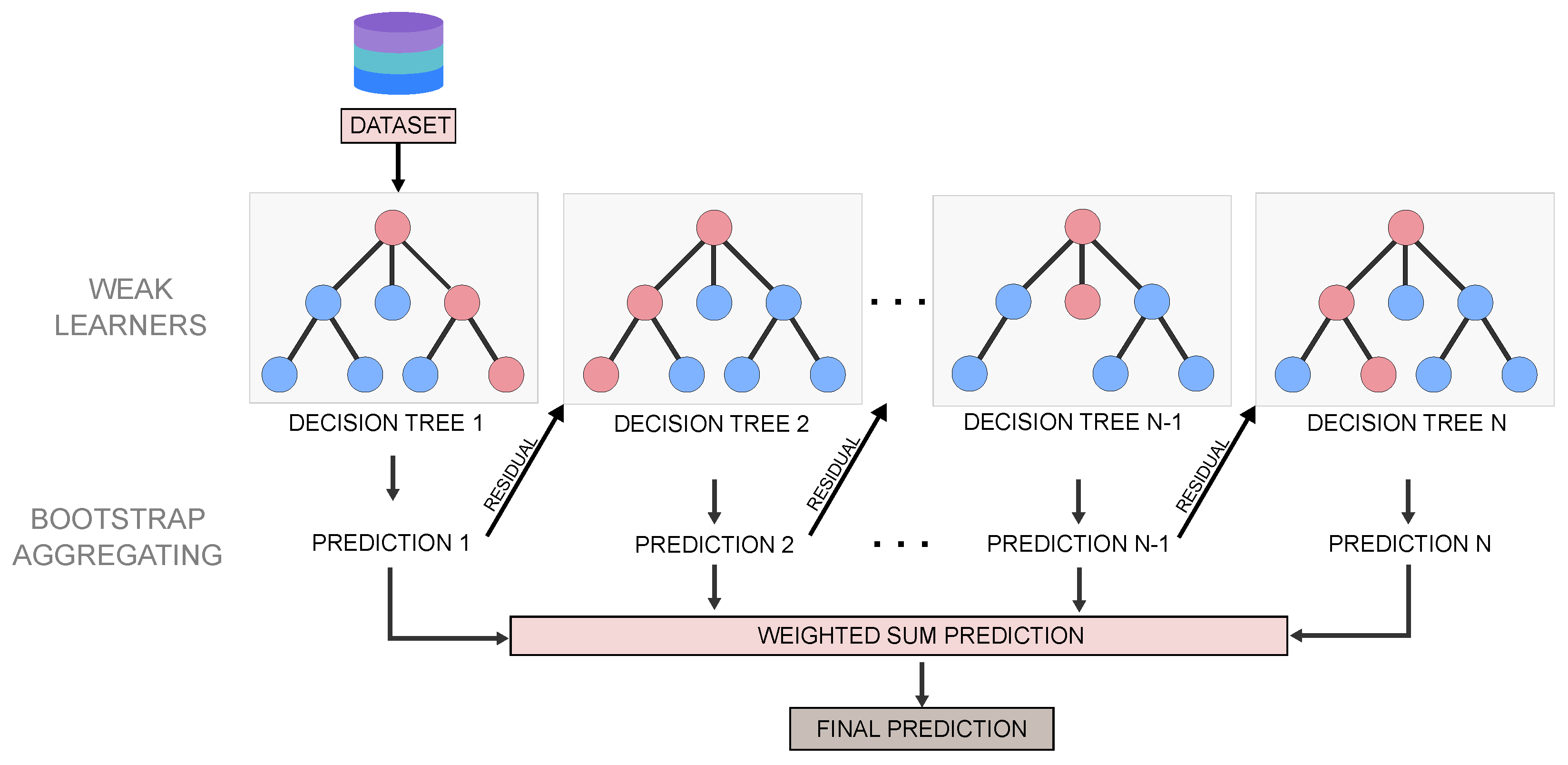
Gradient Boosting is one of the variants of ensemble methods in which multiple weak models (decision trees) are combined to obtain better performance as a whole. Gradient Boosting algorithm was developed by Friedman [
21] and uses decision trees as weak learners. In general, weak learners are not necessary to have the same structure, so they can capture different outputs from the data. In Gradient Boosting, the loss function of each weak learner is minimized using the gradient descent procedure, a global optimisation algorithm which can apply to any loss function that is differentiable. As shown in
Figure 7, the residual (loss error) of the previous tree is taken into account in the training of the following tree. By combining all trees, the final model is able to capture the residual loss from the weak learners.
To better understand how Gradient Boosting works, we present below the steps involved.
- Step 1.
Create a base tree with single root node that acts as the initial guess for all samples.
- Step 2.
Create a new tree from the residual (loss errors) of the previous tree. The new tree in the sequence is fitted to the negative gradient of the loss function with respect to the current predictions.
- Step 3.
Determine the optimal weight of the new tree by minimizing the overall loss function. This weight determines the contribution of the new tree in the final model.
- Step 4.
Scale the tree by learning rate that determines the contribution of the tree in the prediction.
- Step 5.
Combine the new tree with all the previous trees to predict the result and repeat Step 2 until a convergence criterion is satisfied (number of trees exceeds the maximum limit achieved or the new trees do not improve the prediction).
The final prediction model is the weighted sum of the predictions of all the trees involved in the previous procedure, with better-performing trees having a higher weight in the sequence.
In Gradient Boosting, every tree is built one at a time, whereas Random Forests build each tree independently. Thus, the Gradient Boosting algorithm runs in a fixed order, and that sequence cannot change, leading to only sequential evaluation. The Gradient Boosting algorithm is not known for being easy to read or interpret compared to other ensemble algorithms like Random Forest. The combination of trees in Gradient Boosting can be more complex and harder to interpret, although recent developments can improve the interpretability of such complex models. Gradient Boosting is sensitive to outliers since every estimator is obliged to fix the errors in the predecessors. Furthermore, the fact that every estimator bases its correctness on the previous predictors, makes the procedure difficult to scale up.
Overall, Gradient Boosting can be more accurate (under conditions depending on the nature of the problem and the dataset) than Random Forest, due to the sequential nature of the training process of trees which correct each other’s errors. This attribute is capable of capturing complex patterns in the dataset, but it can still be prone to overfitting in noisy datasets.
4.4. CatBoost Regressor (CB)
CatBoost is a relatively new open-source machine learning algorithm which is based on Gradient Boosted decision trees. CatBoost was developed by Yandex engineers [
22] and it focuses on categorical variables without requiring any data conversion in the pre-processing. CatBoost builds symmetric trees (each split is on the same attribute), unlike the Gradient Boosting algorithm, by using permutation techniques. This means that in every split, leaves from the previous tree are split using the same condition. The feature-split pair that accounts for the lowest loss is selected and used for all the level’s nodes. The balanced tree architecture decreases the prediction time while controlling overfitting as the structure serves as regularization. CB uses the concept of ordered boosting, a permutation-driven approach to train the model on a subset of data while calculating residuals on another subset. This technique prevents overfitting and the well-known
dataset shift, a challenging situation where the joint distribution of features and targets differs between the training and test phases.
CatBoost supports all kinds of features, such as numeric, categorical, or text, which reduces the time of the dataset preprocessing phase. It is powerful enough to find any non-linear relationship between the model target and features and has great usability that can deal with missing values, outliers, and high cardinality categorical values on features without any special treatment. Overall, CatBoost is a powerful Gradient Boosting framework that can handle categorical features, missing values, and overfitting issues. It is fast, scalable, and provides good interpretability.
5. ML Pipelines and Performance Results
The ML models developed in this study are based on the dataset described in
Section 3 and make use of the following open-source Python libraries, scikit-learn (RR, RF, GB) [
23] and CatBoost (CB) [
22]. Three different ML models are considered for predicting the fundamental eigenperiod (
), the horizontal displacement at the top story (
), and the normalized shear base over the mass of each story (
) of a shear building. The features of all models are the number of stories (Stories), the normalized stiffness over the mass of each story (
) and the Ground Type.
5.1. Cross Validation and Hyperparameter Tuning
The dataset is split into training and testing set, with 80% and 20% of the samples, respectively. The training set was validated via the k-fold cross-validation method as follows. Data are shuffled and divided into k equal sized subsamples. One of the k subsamples is used as a test (validation) set and the remaining subsamples are put together to be used as training data. Then a model is fitted using training data and evaluated using the test set. The process is repeated k times until each group has served as the validation set. The k results from each model are averaged to obtain the final estimation.
The advantage of the k-fold cross-validation method is that the bias and variance are significantly reduced, while the robustness of the model is increased. The testing set, with data that remain unseen by the models during the training, is used for the final test of the model performance and generalization. With the term generalization we refer to the model’s ability to adapt properly to new, previously unseen data, drawn from the same distribution as the one used to create the model. The value of k depends on the size of the dataset in a way which does not increase the computational cost. In this study, the k value is set equal to 10.
Cross validation is performed together with the hyperparameter tuning in the data pipeline. Hyperparameter tuning is the process of selecting the optimized values for a model’s parameters that maximize its accuracy. The optimal values of the hyperparameters for each model are found using extensive grid search, in which every possible combination of hyperparameters is examined to find the best model. The optimized values of the hyperparameters, along with the range of each ML model and algorithm, are presented in
Table 2. The hyperparameter names correspond to those in the utilized Python libraries [
23]. The hyperparameters not shown had been assigned the default values.
Table 3 collects statistics of the fit time and test score for each model during the cross-validation and hyperparameter tuning process, which is performed on the same hardware configuration. It is shown that Ridge Regression has the lowest fit time for all the models (up to 395 speed-up when compared to the slowest), while CatBoost algorithm outperforms all the others in terms of scoring and exhibits the lowest standard deviation value.
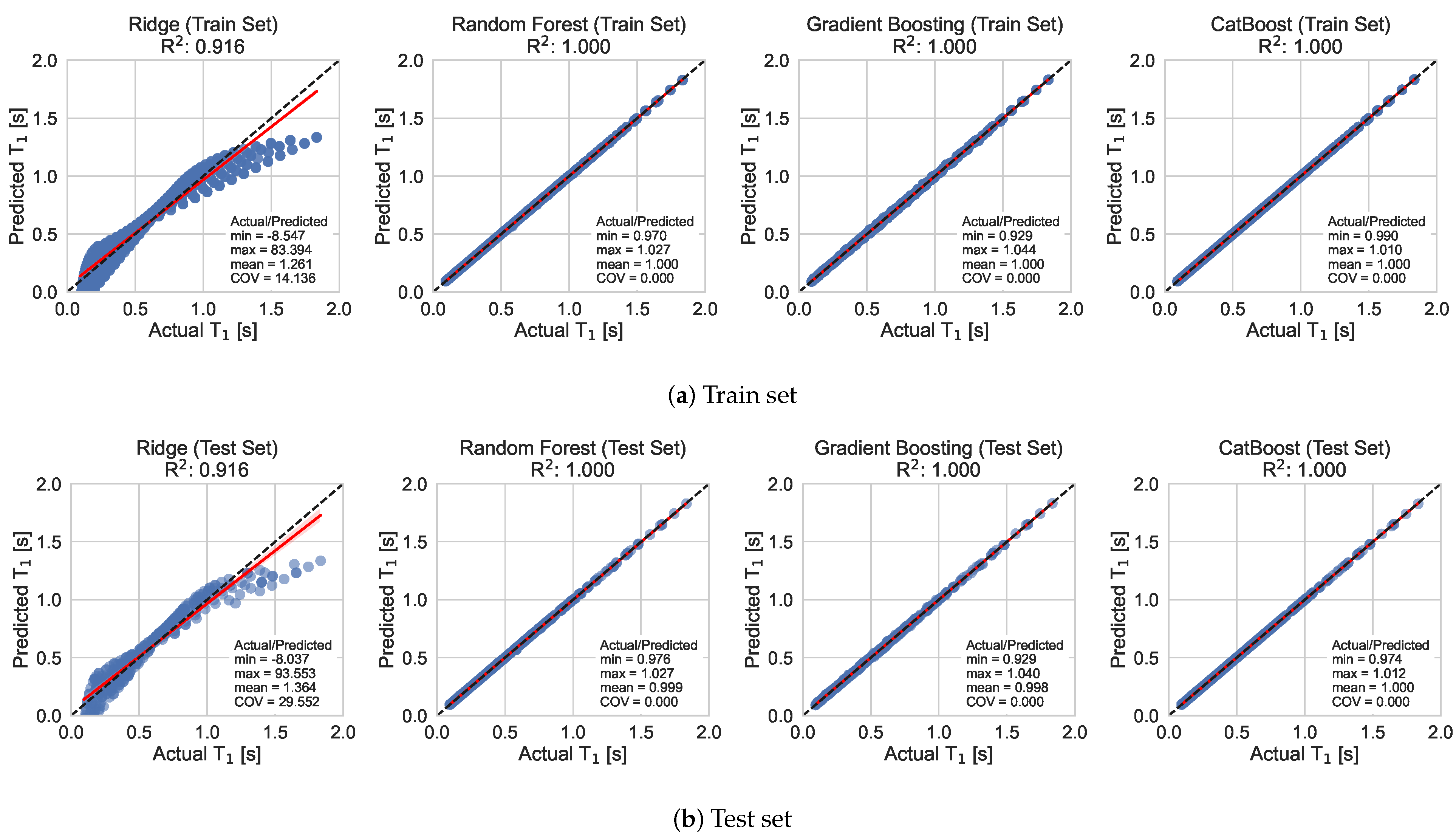
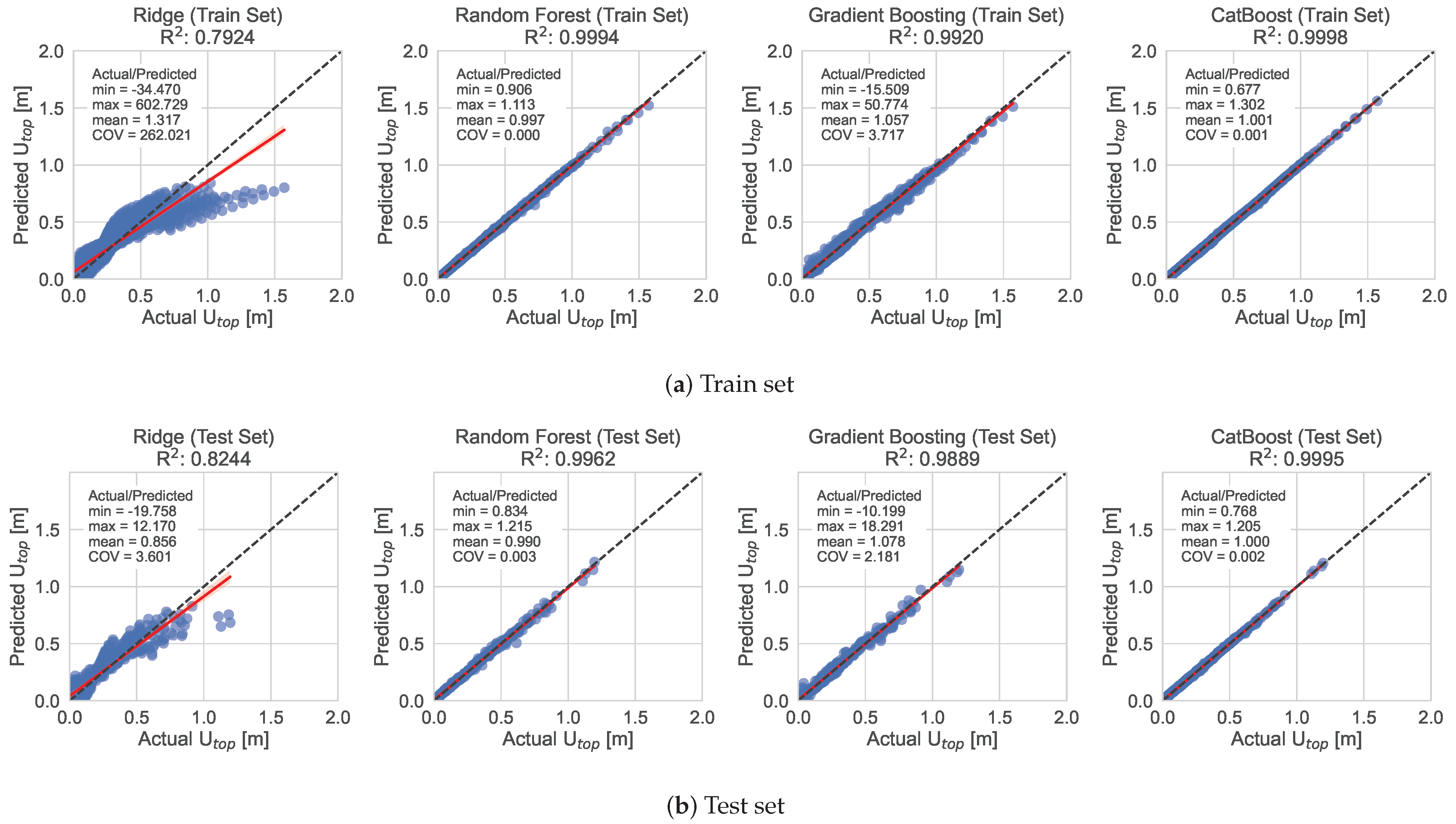
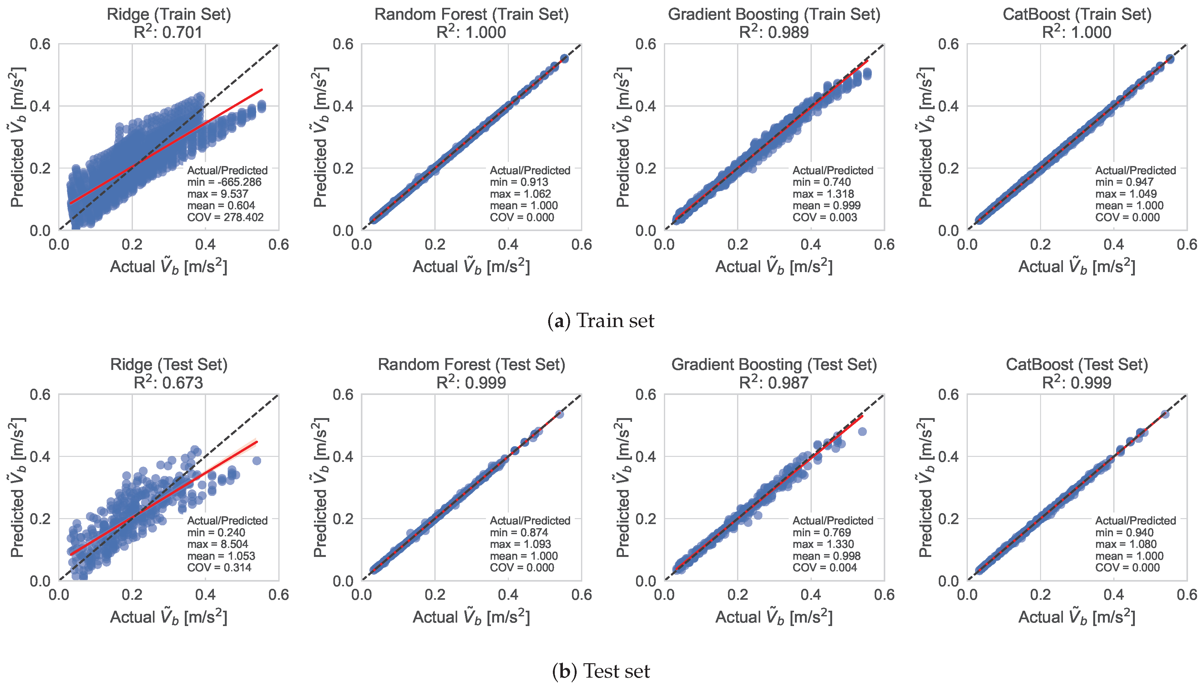
Figure 8,
Figure 9 and
Figure 10 show the performance of the ML models for predicting the
,
and
of the shear buildings in the train and test datasets for the optimized hyperparameter values, accordingly. In general, the ensemble methods achieved higher accuracy compared to the Ridge Regression algorithm. However, the Ridge Regression algorithm managed to achieve acceptable results in the case of the
model.
5.2. Model Evaluation Metrics
To quantify the performance of the ML models, the well-known metrics
,
,
, and
are used [
24]. The definition of each metric is as follows
where
m is the size of the dataset,
and
are the actual and predicted feature value for observation
i, respectively.
The performance metrics of each ML algorithm and model are provided in
Table 4. CatBoost and Random Forest were the two best-performing ML algorithms. CatBoost performed best for the fundamental eigenperiod
, and the horizontal displacement at the top
, with MAE values of 0.008 and 0.0034, respectively, for the test set, compared to 0.0013 and 0.0084 of the Random Forest. On the other hand, Random Forest had the best performance for the normalized base shear force over the mass of each story
, with MAE value of 0.0010 for the test set, compared to 0.0020 of the CatBoost algorithm. The other two algorithms, Ridge and Gradient Boosting showed larger values of MAE as well as worse values for the other metrics.
In general, CatBoost comes first in accuracy with acceptable fit and predicted times for most of the cases, while Ridge Regression takes the trophy for being the fastest to fit the data. Overall, CatBoost appears to be the best model to move forward with, as it came first for, arguably, the most important metrics, although for the case of model, the Random Forest algorithm exhibited slightly better performance.
7. Test Case Scenarios
We consider three test case scenarios for testing the effectiveness of the developed models and, in particular, the selected CatBoost prediction model. The first is a 3-story building, followed by a 8-story building and a 15-story building. The feature values for each scenario are presented in
Table 5. The normalized stiffness (
) for each scenario is 2098.21, 5135.14, and 7169.81 s
, respectively. For practical reasons, we prefer to take
k and
m as independent parameters in the beginning and then calculate
, instead of working with
from start, but it is essentially the same.
The results are presented in
Table 6 for the three outputs, i.e., the fundamental period
, the displacement of the top story
and the base shear force
, for each scenario. In all cases, the prediction model managed to give results of very high precision with error values less than 3%. The maximum error value is only 2.93% corresponding to the shear force for the first scenario. It has to be noted that the model gives
, the normalized base shear force over the mass of each story of the building. By multiplying this with the mass
m, we obtain the last column of the table which corresponds to the final base shear force
.
9. Conclusions
This paper presented the assessment of several ML algorithms for predicting the dynamic response of multi-story shear buildings. A large dataset of dynamic response analyses results was generated through standard sampling methods and conventional response spectrum modal analysis procedures of multi-DOF structural systems. Then, an extensive hyperparameter search was performed to assess the performance of each algorithm and identify the best among them. Of the algorithms examined, CatBoost came first in accuracy with acceptable fit and predicted times for most of the cases, while Ridge Regressor took the trophy for being the fastest to fit the data. Overall, CatBoost appeared to be the best performing algorithm, although for the case of the normalized shear base model, the Random Forest algorithm exhibited slightly better performance.
The results of this study show that ML algorithms, and in particular CatBoost, can successfully predict the dynamic response of multi-story shear buildings, outperforming traditional simplified methods used in engineering practice in terms of speed, with minimal prediction errors. The work demonstrates the potential of ML techniques to improve seismic performance assessment in civil and structural engineering applications, leading to more efficient and safer designs of buildings and other structures. Overall, the use of ML algorithms in the dynamic analysis of structures is a promising approach to accurately predict the dynamic behavior of complex systems.
The study has also some limitations that need to be highlighted and discussed. First of all, the analysis is only elastic and the behavioral factor q of the design spectrum of EC8 takes the fixed value of 1 throughout the study. In addition, damping has been considered with a fixed value of 5%, while the stiffness and mass of each story remains constant along the height of the building. The extension of the work in order to account for these limitations is a topic of interest which will be investigated in the future by adding extra features to the ML model.


