

A FEM Structural Analysis of a Francis Turbine Blade Parametrized Using Piecewise Bernstein Polynomials
 , , , and
Abstract
:1. Introduction
2. Materials and Methods
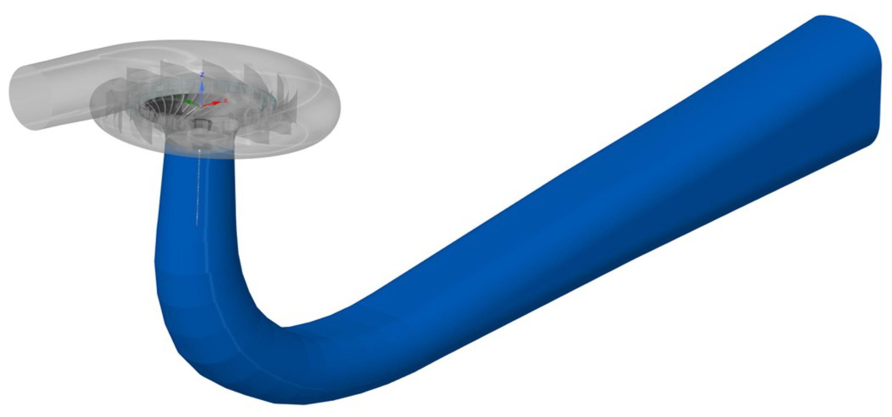
2.1. Blade Description
2.2. Reconstruction Methodology
2.2.1. Data Extraction Stage
2.2.2. Blade Reconstruction Stage
2.2.3. Numerical Blade Evaluation
2.3. Structural Model
2.3.1. Materials
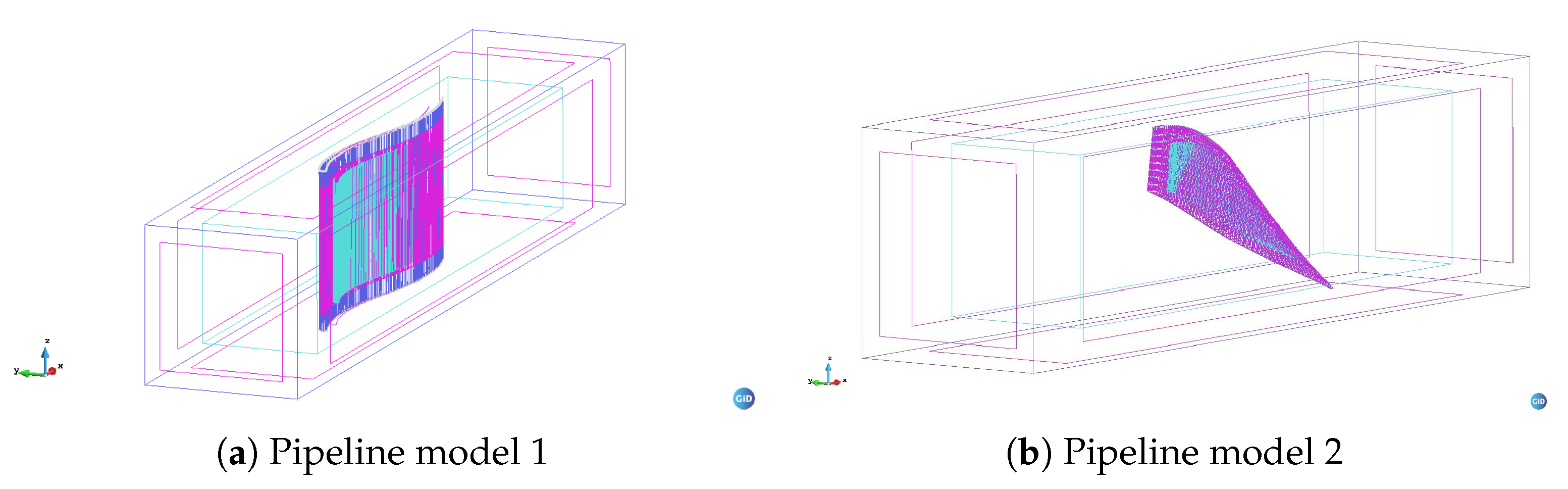
2.3.2. Test Case
- Model 1. A blade with constant cross section generated by extrusion from the Francis blade profile. The pipeline geometry is m long and has a square section of m × 0.15 m (Figure 9a). This geometry resembles the original test model.
- Model 2. A Francis turbine blade was created using the reconstruction methodology described in the preceding section. For this model, the pipeline geometry was adjusted to wrap the blade Francis geometry, thus having a length of m and a rectangular section of m × 0.22 m (Figure 9b).
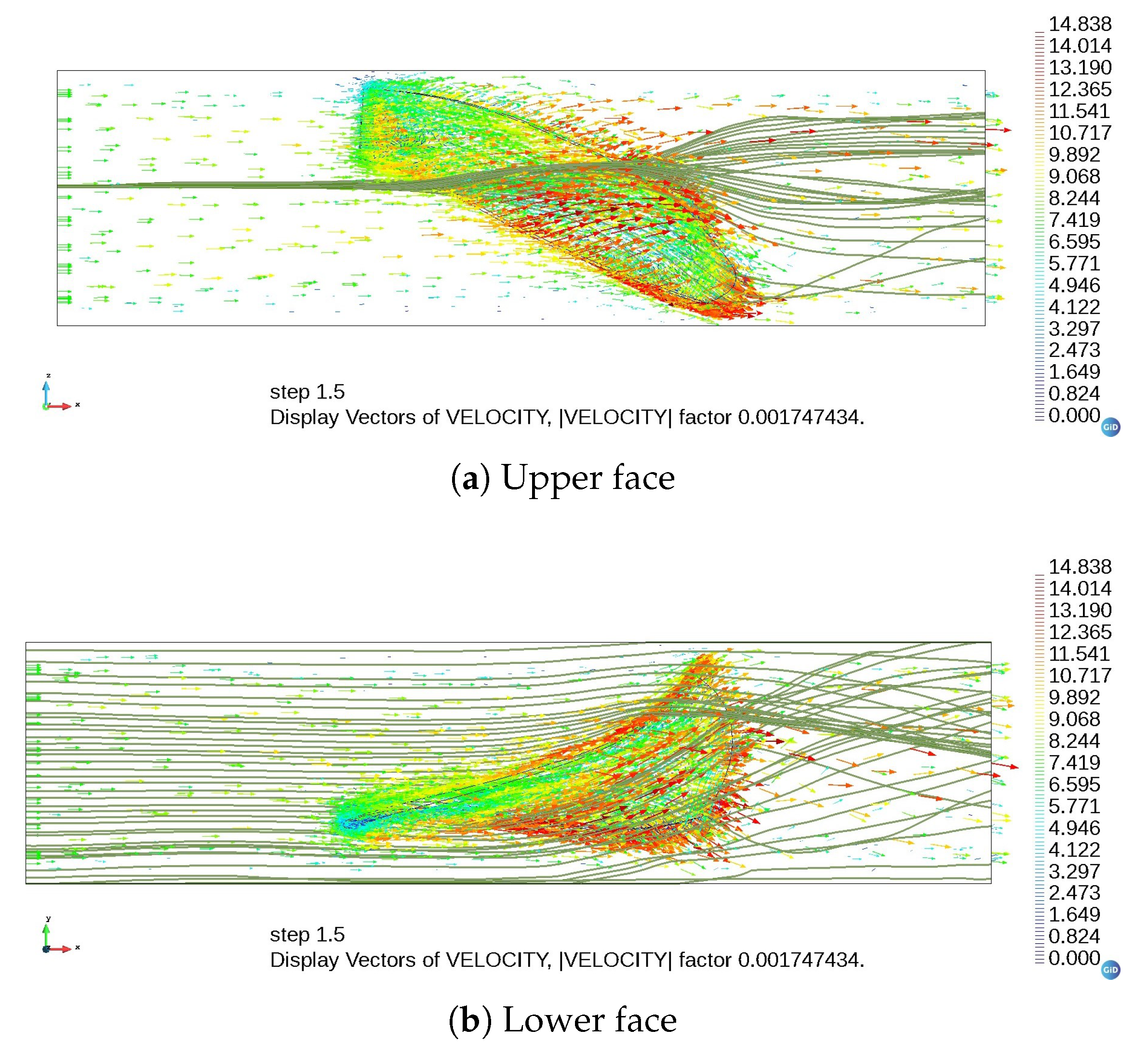
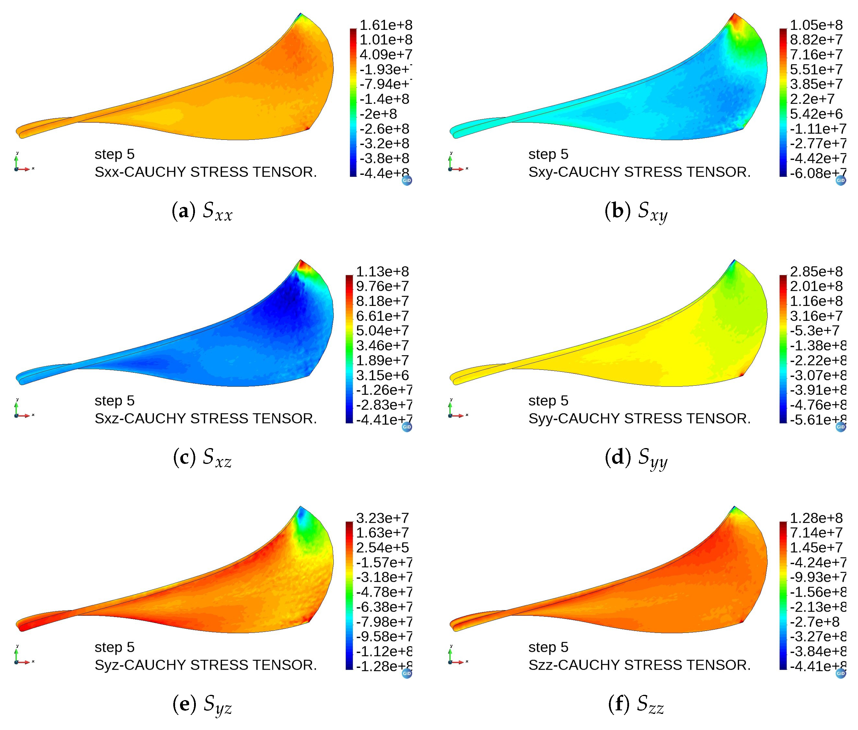
3. Results
4. Discussion
5. Conclusions
Author Contributions
Funding
Informed Consent Statement
Data Availability Statement
Acknowledgments
Conflicts of Interest
Abbreviations
| LE | Leading Edge |
| TE | Trailing Edge |
| NHC | Norwegian Hydropower Center |
| FEM | Finite Element Method |
| XFEM | Extended Finite Element Method |
| LES | Large Eddy Simulation |
| BEP | Best Efficiency Point |
| LTU | Luleå University of Technology |
| PS | Pressure Side |
| SS | Suction Side |
| CFD | Computational Fluid Dynamics |
| NTNU | Norwegian University of Science and Technology |
References
- Cerriteño, A.; Delgado, G.; Galván, S.; Dominguez, F.; Ramírez, R. Reconstruction of the Francis 99 main runner blade using a hybrid parametric approach. In Proceedings of the IOP Conference Series: Earth and Environmental Science, Lausanne, Switzerland, 21–26 March 2021; IOP Publishing: Bristol, UK, 2021; Volume 774, p. 012074. [Google Scholar] [CrossRef]
- Jacomet, A.; Khosravifardshirazi, A.; Sahafnejad-Mohammadi, I.; Dibaj, M.; Javadi, A.A.; Akrami, M. Analysing the influential parameters on the monopile foundation of an offshore wind turbine. Computation 2021, 9, 71. [Google Scholar] [CrossRef]
- Pérez Rubio, L.D.; Galván González, S.R.; Domínguez Mota, F.J.; Cerriteño Sánchez, A.; Tamayo Soto, M.A.; Delgado Sánchez, G. Reconstruction of a Steam Turbine Blade Using Piecewise Bernstein Polynomials and Transfinite Interpolation. In Proceedings of the Turbo Expo: Power for Land, Sea, and Air, Virtual, Online, 7–11 June 2021; American Society of Mechanical Engineers: New York, NY, USA, 2021; Volume 85017, pp. 1–7. [Google Scholar] [CrossRef]
- Agromayor, R.; Anand, N.; Müller, J.D.; Pini, M.; Nord, L.O. A unified geometry parametrization method for turbomachinery blades. Comput. Aided Des. 2021, 133, 102987. [Google Scholar] [CrossRef]
- Farin, G. Curves and Surfaces for Computer-Aided Geometric Design: A Practical Guide, 3rd ed.; Elsevier: Amsterdam, The Netherlands, 2014; pp. 41–62. [Google Scholar]
- Abbott, I.H.; Von Doenhoff, A.E. Theory of Wing Sections: Including a Summary of Airfoil Data, 1st ed.; Courier Corporation: North Chelmsford, MA, USA, 2012; pp. 123–182. [Google Scholar]
- Ferrando, L.; Kueny, J.L.; Avellan, F.; Pedretti, C.; Tomas, L. Surface parameterization of a Francis runner turbine for optimum design. In Proceedings of the 22nd IAHR Symposium on Hydraulic Machinery and Systems, Stockholm, Sweden, 29 June–2 July 2004. [Google Scholar]
- Delgado, G.; Galván, S.; Dominguez-Mota, F.; García, J.; Valencia, E. Reconstruction Methodology of a Francis runner blade using numerical tools. J. Mech. Sci. Technol. 2020, 34, 1237–1247. [Google Scholar] [CrossRef]
- Hasmatuchi, V.; Roth, S.; Botero, F.; Avellan, F.; Farhat, M. High-speed flow visualization in a pump-turbine under off-design operating conditions. In Proceedings of the IOP Conference Series: Earth and Environmental Science, 25th IAHR Symposium on Hydraulic Machinery and Systems, ’Politehnica’, University of Timişoara, Timişoara, Romania, 20–24 September 2010; IOP Publishing: Bristol, UK, 2010; Volume 12, pp. 1–8. [Google Scholar] [CrossRef]
- Brandão, P.; Infante, V.; Deus, A. Thermo-mechanical modeling of a high pressure turbine blade of an airplane gas turbine engine. Procedia Struct. Integr. 2016, 1, 189–196. [Google Scholar] [CrossRef] [Green Version]
- Khalesi, J.; Modaresahmadi, S.; Atefi, G. SEM Gamma prime observation in a thermal and stress analysis of a first-stage Rene’80H gas turbine blade: Numerical and experimental investigation. Iran. J. Sci. Technol. Trans. Mech. Eng. 2019, 43, 613–626. [Google Scholar] [CrossRef]
- Chung, H.; Sohn, H.S.; Park, J.S.; Kim, K.M.; Cho, H.H. Thermo-structural analysis of cracks on gas turbine vane segment having multiple airfoils. Energy 2017, 118, 1275–1285. [Google Scholar] [CrossRef]
- Cai, L.; He, Y.; Wang, S.; Li, Y.; Li, F. Thermal-Fluid-Solid coupling analysis on the temperature and thermal stress field of a Nickel-Base superalloy turbine blade. Materials 2021, 14, 3315. [Google Scholar] [CrossRef]
- Nekahi, S.; Vaferi, K.; Vajdi, M.; Moghanlou, F.S.; Asl, M.S.; Shokouhimehr, M. A numerical approach to the heat transfer and thermal stress in a gas turbine stator blade made of HfB2. Ceram. Int. 2019, 45, 24060–24069. [Google Scholar] [CrossRef]
- Kwon, Y.W.; Bang, H. The Finite Element Method Using MATLAB, 2nd ed.; CRC Press: Boca Raton, FL, USA, 2000; pp. 311–361. [Google Scholar]
- Liu, G.R.; Quek, S.S. The Finite Element Method: A Practical Course, 2nd ed.; Butterworth-Heinemann: Oxford, UK, 2013; pp. 199–232. [Google Scholar]
- Zienkiewicz, O.C.; Taylor, R.L.; Zhu, J.Z. The Finite Element Method: Its Basis and Fundamentals, 6th ed.; Elsevier: Amsterdam, The Netherlands, 2005; pp. 187–253. [Google Scholar]
- Vasilyev, B. Stress–Strain State Prediction of High-Temperature Turbine Single Crystal Blades Using Developed Plasticity and Creep Models. In Proceedings of the Turbo Expo: Power for Land, Sea, and Air, Düsseldorf, Germany, 16–20 June 2014; American Society of Mechanical Engineers: New York, NY, USA, 2014; Volume 45769. [Google Scholar] [CrossRef]
- Ahmed, S.H.; Husain, G.; Abdulrazaq, M.A. Theoretical Stress Analysis of Gas Turbine Blade Made From Different Alloys. Al-Rafidain Eng. J. 2019, 24, 10–18. [Google Scholar] [CrossRef]
- Kauss, O.; Tsybenko, H.; Naumenko, K.; Hütter, S.; Krüger, M. Structural analysis of gas turbine blades made of Mo-Si-B under transient thermo-mechanical loads. Comput. Mater. Sci. 2019, 165, 129–136. [Google Scholar] [CrossRef]
- Liu, X.; Luo, Y.; Wang, Z. A review on fatigue damage mechanism in hydro turbines. Renew. Sustain. Energy Rev. 2016, 54, 1–14. [Google Scholar] [CrossRef]
- Seidel, U.; Mende, C.; Hübner, B.; Weber, W.; Otto, A. Dynamic loads in Francis runners and their impact on fatigue life. In Proceedings of the IOP conference series: Earth and environmental science, Montreal, QC, Canada, 22–26 September 2014; IOP Publishing: Bristol, UK, 2021; Volume 22, p. 032054. [Google Scholar] [CrossRef] [Green Version]
- Zuo, Z.; Liu, S.; Sun, Y.; Wu, Y. Pressure fluctuations in the vaneless space of High-head pump-turbines—A review. Renew. Sustain. Energy Rev. 2015, 41, 965–974. [Google Scholar] [CrossRef]
- Claudio, R.; Branco, C.; Gomes, E.; Byrne, J. Life prediction of a gas turbine disc using the finite element method. 8AS Jornadas Fract. 2002, 131–144. [Google Scholar] [CrossRef]
- Keck, H.; Sick, M. Thirty years of numerical flow simulation in hydraulic turbomachines. Acta Mech. 2008, 201, 211–229. [Google Scholar] [CrossRef]
- Chirag, T.; Cervantes, M.J.; Bhupendrakumar, G.; Dahlhaug, O.G. Pressure measurements on a high-head Francis turbine during load acceptance and rejection. J. Hydraul. Res. 2014, 52, 283–297. [Google Scholar] [CrossRef]
- Platonov, D.; Minakov, A.; Sentyabov, A. Numerical investigation of hydroacoustic pressure pulsations due to rotor-stator interaction in the Francis-99 turbine. In Proceedings of the Journal of Physics: Conference Series, NTNU, Trondheim, Norway, 28–29 May 2019; IOP Publishing: Bristol, UK, 2021; Volume 1296, p. 012009. [Google Scholar] [CrossRef]
- Sukumar, N.; Moës, N.; Moran, B.; Belytschko, T. Extended finite element method for three-dimensional crack modelling. Int. J. Numer. Methods Eng. 2000, 48, 1549–1570. [Google Scholar] [CrossRef]
- Schwerdt, L.; Hauptmann, T.; Kunin, A.; Seume, J.R.; Wallaschek, J.; Wriggers, P.; Panning-von Scheidt, L.; Löhnert, S. Aerodynamical and structural analysis of operationally used turbine blades. Procedia CIRP 2017, 59, 77–82. [Google Scholar] [CrossRef] [Green Version]
- Kim, Y.; Cho, H.; Park, S.; Kim, H.; Shin, S. Advanced structural analysis based on reduced-order modeling for gas turbine blade. AIAA J. 2018, 56, 3369–3373. [Google Scholar] [CrossRef]
- Cox, K.; Echtermeyer, A. Structural design and analysis of a 10MW wind turbine blade. Energy Procedia 2012, 24, 194–201. [Google Scholar] [CrossRef] [Green Version]
- Griffin, D.A. Blade System Design Studies Volume II: Preliminary Blade Designs and Recommended Test Matrix; Technical Report; Sandia National Laboratories (SNL): Albuquerque, NM, USA; Livermore, CA, USA,, 2004. [CrossRef] [Green Version]
- Castorrini, A.; Corsini, A.; Rispoli, F.; Venturini, P.; Takizawa, K.; Tezduyar, T.E. Computational analysis of wind-turbine blade rain erosion. Comput. Fluids 2016, 141, 175–183. [Google Scholar] [CrossRef]
- Castorrini, A.; Corsini, A.; Rispoli, F.; Venturini, P.; Takizawa, K.; Tezduyar, T.E. SUPG/PSPG computational analysis of rain erosion in wind-turbine blades. In Advances in Computational Fluid-Structure Interaction and Flow Simulation: New Methods and Challenging Computations; Birkhäuser: Basel, Switzerland, 2016; pp. 77–96. [Google Scholar] [CrossRef]
- Kumar, R.R.; Pandey, K. Static structural and modal analysis of gas turbine blade. In Proceedings of the IOP Conference series: Materials science and engineering, Narsimha Reddy Engineering College, Hyderabad, India, 3–4 July 2017; IOP Publishing: Bristol, UK, 2021; Volume 225. [Google Scholar] [CrossRef]
- Čupr, P.; Štefan, D.; Habán, V.; Rudolf, P. FSI analysis of francis-99 hydrofoil employing SBES model to adequately predict vortex shedding. In Proceedings of the Francis-99: Fluid Structure Interactions in Francis Turbines, Trondheim, Norway, 28–29 May 2019; IOP Publishing: Bristol, UK, 2021; Volume 1296, p. 012002. [Google Scholar] [CrossRef] [Green Version]
- Trivedi, C.; Cervantes, M.J.; Dahlhaug, O.G. Experimental and numerical studies of a high-head Francis turbine: A review of the Francis-99 test case. Energies 2016, 9, 1–24. [Google Scholar] [CrossRef] [Green Version]
- Østby, P.T.; Agnalt, E.; Haugen, B.; Billdal, J.T.; Dahlhaug, O.G. Fluid structure interaction of Francis-99 turbine and experimental validation. In Proceedings of the Francis-99: Fluid Structure Interactions in Francis Turbines, NTNU, Trondheim, Norway, 28–29 May 2019; IOP Publishing: Bristol, UK, 2021; Volume 1296, p. 012006. [Google Scholar] [CrossRef]
- Trivedi, C.; Agnalt, E.; Dahlhaug, O.G. Investigations of unsteady pressure loading in a Francis turbine during variable-speed operation. Renew. Energy 2017, 113, 397–410. [Google Scholar] [CrossRef]
- Sagmo, K.; Storli, P. A test of the v2-f k-ϵ turbulence model for the prediction of vortex shedding in the Francis-99 hydrofoil test case. In Proceedings of the Journal of Physics: Conference Series, NTNU, Trondheim, Norway, 28–29 May 2019; IOP Publishing: Bristol, UK, 2019; Volume 1296, p. 012004. [Google Scholar] [CrossRef]
- Norwegian Hydropower Centre. 2016. Available online: https://www.ntnu.edu/nvks/norwegian-hydropower-center (accessed on 16 March 2023).
- Dubé, J.F.; Guibault, F.; Vallet, M.G.; Trépanier, J.Y. Turbine blade reconstruction and optimization using subdivision surfaces. In Proceedings of the 44th AIAA Aerospace Sciences Meeting and Exhibit, Reno, NV, USA, 9–12 January 2006; p. 1327. [Google Scholar] [CrossRef]
- Sripawadkul, V.; Padulo, M.; Guenov, M. A comparison of airfoil shape parameterization techniques for early design optimization. In Proceedings of the 13th AIAA/ISSMO Multidisciplinary Analysis Optimization Conference, Fort Worth, TX, USA, 13–15 September 2010; p. 9050. [Google Scholar] [CrossRef]
- Oliver Olivella, X.; Agelet de Saracibar Bosch, C. Continuum Mechanics for Engineers. Theory and Problems, 2nd ed.; 2017; pp. 369–419. [Google Scholar] [CrossRef]
- Owen, D.; Hinton, E. Finite Element in Plasticity: Theory and Practice, 1st ed.; Pineridge Press Limited: Swansea, UK, 1980; pp. 209–278. [Google Scholar]
- de Souza Neto, E.A.; Peric, D.; Owen, D.R. Computational Methods for Plasticity: Theory and Applications, 1st ed.; John Wiley & Sons: Hoboken, NJ, USA, 2011; pp. 104–215. [Google Scholar]
- Barbu, L.G.; Cornejo, A.; Martínez, X.; Oller, S.; Barbat, A. Methodology for the analysis of post-tensioned structures using a constitutive serial-parallel rule of mixtures: Large scale non-linear analysis. Compos. Struct. 2019, 216, 315–330. [Google Scholar] [CrossRef]
- Jiménez, S.; Cornejo, A.; Barbu, L.G.; Barbat, A.; Oller, S. Failure pressure analysis of a nuclear reactor prestressed concrete containment building. Eng. Struct. 2021, 236, 112052. [Google Scholar] [CrossRef]
- Simo, J.C.; Hughes, T.J. Computational Inelasticity, 2nd ed.; Springer: Berlin, Germany, 1998; pp. 71–110. [Google Scholar]
- Elsherif, D.M.; Abd El-Wahab, A.A.; Abdellatif, M.H. Factors affecting stress distribution in wind turbine blade. In Proceedings of the IOP Conference Series: Materials Science and Engineering, Cairo, Egypt, 9–11 April 2019; IOP Publishing: Bristol, UK, 2019; Volume 610, p. 012020. [Google Scholar] [CrossRef]
- Gupta, S. Fluid Mechanics and Hydraulic Machines, 1st ed.; Pearson Education India: New Delhi, India, 2006; pp. 206–249. [Google Scholar]
- Zorrilla Martínez, R. FSI Procedures for Civil Engineering Applications. Master’s Thesis, Universitat Politècnica de Catalunya, Barcelona, Spain, 2016. [Google Scholar]
- Codina, R. Pressure stability in fractional step finite element methods for incompressible flows. J. Comput. Phys. 2001, 170, 112–140. [Google Scholar] [CrossRef]
- Codina, R. A stabilized finite element method for generalized stationary incompressible flows. Comput. Methods Appl. Mech. Eng. 2001, 190, 2681–2706. [Google Scholar] [CrossRef]
- Codina, R. Stabilized finite element approximation of transient incompressible flows using orthogonal subscales. Comput. Methods Appl. Mech. Eng. 2002, 191, 4295–4321. [Google Scholar] [CrossRef]
- Ribó, R.; Pasenau, M.; Escolano, E.; Coll, A.; Melendo, A.; Monros, A.; Gárate, J.; Peyrau, M. GiD Reference Manual; Technical Report; CIMNE: Barcelona, Spain, 2022. [Google Scholar]


| Property | Magnitud | Unit |
|---|---|---|
| Young’s Modulus | 71,000 | MPa |
| Poisson’s Ratio | 0.33 | |
| Density | 2770 | kg/m |
| Yield Strength | 280 | MPa |
| Tensile Ultimate Strength | 310 | MPa |
| Bulk Modulus | 69,608 | MPa |
| Shear Modulus | 26,692 | MPa |
| Ultimate Bearing Strength | 669 | MPa |
| Time (s) | Hydrofoil Test (kPa) | Model 1 (kPa) | Model 2 (kPa) |
|---|---|---|---|
| 0.0 | 659.5 | 0.0 | 0.0 |
| 1.0 | 666.8 | 13.5 | 31.7 |
| 1.6 | 675.2 | 31.1 | 80.0 |
| 2.0 | 683.7 | 46.6 | 123.7 |
| 3.0 | 710.0 | 97.4 | 278.5 |
| 4.0 | 747.3 | 163.9 | 504.5 |
| 5.0 | 794.2 | 244.7 | 773.0 |
Disclaimer/Publisher’s Note: The statements, opinions and data contained in all publications are solely those of the individual author(s) and contributor(s) and not of MDPI and/or the editor(s). MDPI and/or the editor(s) disclaim responsibility for any injury to people or property resulting from any ideas, methods, instructions or products referred to in the content. |
© 2023 by the authors. Licensee MDPI, Basel, Switzerland. This article is an open access article distributed under the terms and conditions of the Creative Commons Attribution (CC BY) license (https://creativecommons.org/licenses/by/4.0/).
Share and Cite
Arias-Rojas, H.; Rodríguez-Velázquez, M.A.; Cerriteño-Sánchez, Á.; Domínguez-Mota, F.J.; Galván-González, S.R. A FEM Structural Analysis of a Francis Turbine Blade Parametrized Using Piecewise Bernstein Polynomials. Computation 2023, 11, 123. https://doi.org/10.3390/computation11070123
Arias-Rojas H, Rodríguez-Velázquez MA, Cerriteño-Sánchez Á, Domínguez-Mota FJ, Galván-González SR. A FEM Structural Analysis of a Francis Turbine Blade Parametrized Using Piecewise Bernstein Polynomials. Computation. 2023; 11(7):123. https://doi.org/10.3390/computation11070123
Chicago/Turabian StyleArias-Rojas, Heriberto, Miguel A. Rodríguez-Velázquez, Ángel Cerriteño-Sánchez, Francisco J. Domínguez-Mota, and Sergio R. Galván-González. 2023. "A FEM Structural Analysis of a Francis Turbine Blade Parametrized Using Piecewise Bernstein Polynomials" Computation 11, no. 7: 123. https://doi.org/10.3390/computation11070123