On the Time Frequency Compactness of the Slepian Basis of Order Zero for Engineering Applications

Abstract

Time and frequency concentrations of waveforms are often of interest in engineering applications. The Slepian basis of order zero is an index-limited (finite) vector that is known to be optimally concentrated in the frequency domain. This paper proposes a method of mapping the index-limited Slepian basis to a discrete-time vector, hence obtaining a time-limited, discrete-time Slepian basis that is optimally concentrated in frequency. The main result of this note is to demonstrate that the (discrete-time) Slepian basis achieves minimum time-bandwidth compactness under certain conditions. We distinguish between the characteristic (effective) time/bandwidth of the Slepians and their defining time/bandwidth (the time and bandwidth parameters used to generate the Slepian basis). Using two different definitions of effective time and bandwidth of a signal, we show that when the defining time-bandwidth product of the Slepian basis increases, its effective time-bandwidth product tends to a minimum value. This implies that not only are the zeroth order Slepian bases known to be optimally time-limited and band-concentrated basis vectors, but also as their defining time-bandwidth products increase, their effective time-bandwidth properties approach the known minimum compactness allowed by the uncertainty principle. Conclusions are also drawn about the smallest defining time-bandwidth parameters to reach the minimum possible compactness. These conclusions give guidance for applications where the time-bandwidth product is free to be selected and hence may be selected to achieve minimum compactness.

1. Introduction

Compact waveforms are often desired in engineering applications, such as communications, signal processing, and detecting or imaging systems [1,2,3,4,5,6,7]. Slepian, Landau, and Pollak provided a comprehensive study of time and frequency concentration problems [8,9,10,11,12], leading to the introduction of Prolate Spheroidal Wave Functions (PSWF) and Discrete Prolate Spheroidal Sequences (DPSS) as functions and sequences with optimal time-frequency concentration properties. The Slepian basis are vectors defined on a discrete index, obtained by truncating the infinite length Discrete Prolate Spheroidal Sequence. The PSWFs answer the question, “what is the maximum concentration of a bandlimited function inside a given interval?”. Similarly, the DPSS answer the question, “what is the maximum concentration of a bandlimited function within a finite index set?”. We note that the literature often uses the terms DPSS and ‘Slepian basis’ interchangeably; however the terminology we adopt in this paper is to denote the infinite length vectors as DPSS and finite length (index-limited) vectors as Slepian basis vectors.

Although the PSWF, DPSS and Slepian bases are known to have optimal concentration properties given a hard limit in the opposite domain [13], their overall time/frequency compactness is not well studied. To complicate matters further, a signal’s compactness can be evaluated in various ways [9]; for example, Gaussian functions are the most compact waveform under certain definitions of time and bandwidth compactness [14]. Hence, Slepian bases may not be the most compact waveform under measurements of compactness required for various engineering applications. Furthermore, it is also not clear how to choose the most compact Slepian from the set of Slepians. This communication paper considers the compactness properties of the Slepians under different definitions of compactness. This paper proposes a method of mapping the index-limited Slepian basis to a discrete-time vector, hence obtaining a time-limited (discrete-time) Slepian basis. Furthermore, the time-frequency compactness properties of the time-limited Slepian bases are discussed, and some conclusions are made.

The Slepian basis is a set of index-limited vectors that are optimally concentrated in the frequency domain [12]. The Slepian basis $s_0,\dots ,s_{N-1}\in {ℝ}^N$ are the orthonormal eigenvectors of the matrix $B\in {ℝ}^{N\times N}$ given by [13]

$$B\left[m,n\right]=\left\{\begin{array}{cc}\frac{\sin \left[2\pi \sigma \left(m-n\right)\right]}{\pi \left(m-n\right)}\hfill & \hspace{0.33em}\hspace{0.17em}\hspace{0.17em}\hspace{0.33em}\hspace{0.33em}\hspace{0.33em}m\ne n\\ \hspace{0.33em}\hspace{0.17em}2\sigma \hfill & \hspace{0.33em}\hspace{0.17em}\hspace{0.17em}\hspace{0.33em}\hspace{0.33em}\hspace{0.33em}m=n\end{array}\right.\hspace{0.33em}\hspace{0.33em}\hspace{0.33em}\mathrm{for}\hspace{0.17em}\hspace{0.17em}m,n=0,\dots ,N-1$$

(1)

The matrix B is known in the literature as the prolate matrix [15]. In Equation (1), $0<\sigma <\raisebox{1ex}{$1$}\!\left/ \!\raisebox{-1ex}{$2$}\right.$ is the bandwidth of the Slepian basis. The Slepian basis used in this paper is obtained through MATLAB R2019b signal processing toolbox function dpss, which calculates the eigenvalues and eigenvectors of the prolate matrix using a fast autocorrelation technique [16]. The prolate matrix is known to be generally ill-conditioned and this fast autocorrelation approach gives numerically superior results compared to using simpler brute-force approaches.

2. Materials and Methods

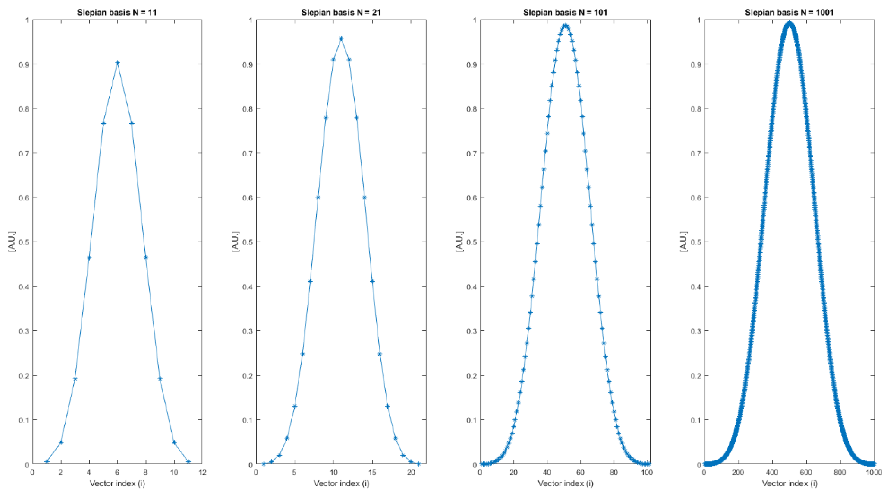
In this section, we demonstrate the mapping of the Slepian basis to a discrete-time vector and present approaches to quantify the effective time and bandwidth of the signal.

2.1. Slepian Basis

The Slepian basis is a function of number of points N and time bandwidth product. In this paper, in order to exploit symmetry of intervals and of definitions of the Fourier transform, the defining duration of waveforms will be considered as $\left[-T,T\right]$ in time, and $\left[-B,B\right]$ in frequency, where B is in Hertz. As a comment, Matlab refers to the time (length of the interval; in this paper 2T), and half-bandwidth (in this paper B) product $c=2TB$. However, the Matlab “time half-bandwidth” nomenclature is not common in the literature, which more commonly refers to a “time bandwidth” product. We draw this to the attention of the reader since there are various slightly different definitions of time-bandwidth product used in the literature in general, and in the literature on DPSS and PSWFs specifically.

The zeroth order Slepian basis vector $s_0\left(N,c\right)$ is the eigenvector corresponding to the largest eigenvalue of the prolate matrix defined by parameters N and c, here defined as the vectors returned by the Matlab function dpss written by E. Breitenberger [16]. N is the size of the vector and must be greater than 2c + 1 with no upper limit. The vector returned can be mapped to a time vector $t=-T_S:dt:T_S$ with $dt=\frac{2T_S}{N-1}$, where 2T_S is the duration of the Slepian basis. That is, we choose c and N, then the dpss function solves the prolate matrix (Equation 1) eigenvalue problem for $\sigma =\frac{c}{N-1}$ to return a Slepian basis. This is achieved by using inverse iteration with the exact eigenvalues on a starting vector with approximate shape, to obtain the eigenvectors required. The eigenvalues of the Toeplitz sinc matrix are then computed using a fast autocorrelation technique. The N-dimensional eigenvector corresponding to the largest eigenvalue is $s_0\left(N,c\right)$. Now, we choose a $T_S$ to convert any of the Slepian vectors into a discrete-time vector via $t=-T_S:dt:T_S$. The resulting discrete-time Slepian basis vector will be time-limited to $\left[-T_S,T_S\right]$ and optimally concentrated in the bandwidth $\left[-B_S,B_S\right]$ with $B_S=\frac{c}{2T_S}$, where $B_S$ is denoted in Hertz. An example of the Matlab code to generate the Slepian basis with N = 201 and c = 10 is provided in Appendix A. The complete Matlab code to generate the figures in Section 3 is provided in Appendix B and Appendix C.

2.2. Compactness

There are several different ways to quantify the time and frequency compactness characteristics of a discrete-time signal $x_i$ (defined on discrete-time vector $t_i$) and its Fourier transform $X_i$ (defined on discrete frequency vector $f_i$). Heuristically speaking, compactness is a measure of how compact a signal can be, or in other words, how much the signal spreads out. It is known that signals that are compact (narrow) in time cannot be compact in frequency. From the mathematical symmetry of the definitions, the reverse is also true. That is, signals compact (narrow) in frequency cannot be compact in time. We are interested in quantifying the compactness of signals in both time and frequency domains. To consider compactness, we introduce two different definitions. The most common method to quantify compactness—how much a signal is narrow or wide—is by measuring via variance [9,17], defined as

$$T_{\sigma }^2=\frac{{\displaystyle \sum _{i=1}^N{\left(t_i-\overline{t}\right)}^2{\left|x_i\right|}^2}}{{\displaystyle \sum _{i=1}^N{\left|x_i\right|}^2}}$$

(2)

$$B_{\sigma }^2=\frac{{\displaystyle \sum _{i=1}^N{\left(f_i-\overline{f}\right)}^2{\left|X_i\right|}^2}}{{\displaystyle \sum _{i=1}^N{\left|X_i\right|}^2}}$$

(3)

Here, $T_{\sigma }^2$ and $B_{\sigma }^2$ are the variances, and $T_{\sigma }$ and $B_{\sigma }$ are the signal’s variance-based characteristic time and bandwidth, respectively. A smaller $T_{\sigma }$ or $B_{\sigma }$ means the signal has a shorter characteristic duration or narrower bandwidth. Note that the characteristic time and bandwidth are different from the defining time $T_S$ and bandwidth $B_S$. Here, $\overline{t}$ and $\overline{f}$ are the mean values of the time and frequency vectors, $t_i$ and $f_i$, and N is the length of the signal.

Another common method to quantify signal time and frequency compactness characteristics is via the signal energy-based effective time and bandwidth, defined through energy concentration [9,17], given by

$${\alpha }^2=\frac{{\displaystyle \sum _{-T_{{\alpha }^2}}^{T_{{\alpha }^2}}{\left|x_i\right|}^2}}{{\displaystyle \sum _{-\infty }^{\infty }{\left|x_i\right|}^2}}$$

(4)

and

$${\beta }^2=\frac{{\displaystyle \sum _{-B_{{\beta }^2}}^{B_{{\beta }^2}}{\left|X_i\right|}^2}}{{\displaystyle \sum _{-\infty }^{\infty }{\left|X_i\right|}^2}}$$

(5)

where ${\alpha }^2$ and ${\beta }^2$ are measurements of the signal’s energy proportion in a time interval $\left[-T_{{\alpha }^2},T_{{\alpha }^2}\right]$ and frequency interval $\left[-B_{{\beta }^2},B_{{\beta }^2}\right]$, respectively. This paper uses ${\alpha }^2=98\%$ and ${\beta }^2=98\%$ as the criterion to determine a signal’s energy-based effective time and bandwidth. That is, the (energy-based) effective time and bandwidth are the values of time and bandwidth that capture 98% of the signal energy in both time and frequency domains. For example, $T_{98\%}=2s$ implies that 98% of the energy is concentrated in $\left[-T_{98\%},T_{98\%}\right]$.

We use the variance and energy-based effective time/frequency definitions of compactness via $T_{\sigma },B_{\sigma },T_{98\%},B_{98\%}$ to quantify the signal effective time and frequency values. In contrast, the defining time and bandwidth $T_S,B_S$ are those used to define the Slepian basis through the prolate matrix, as discussed in the previous subsection.

3. Results and Discussion

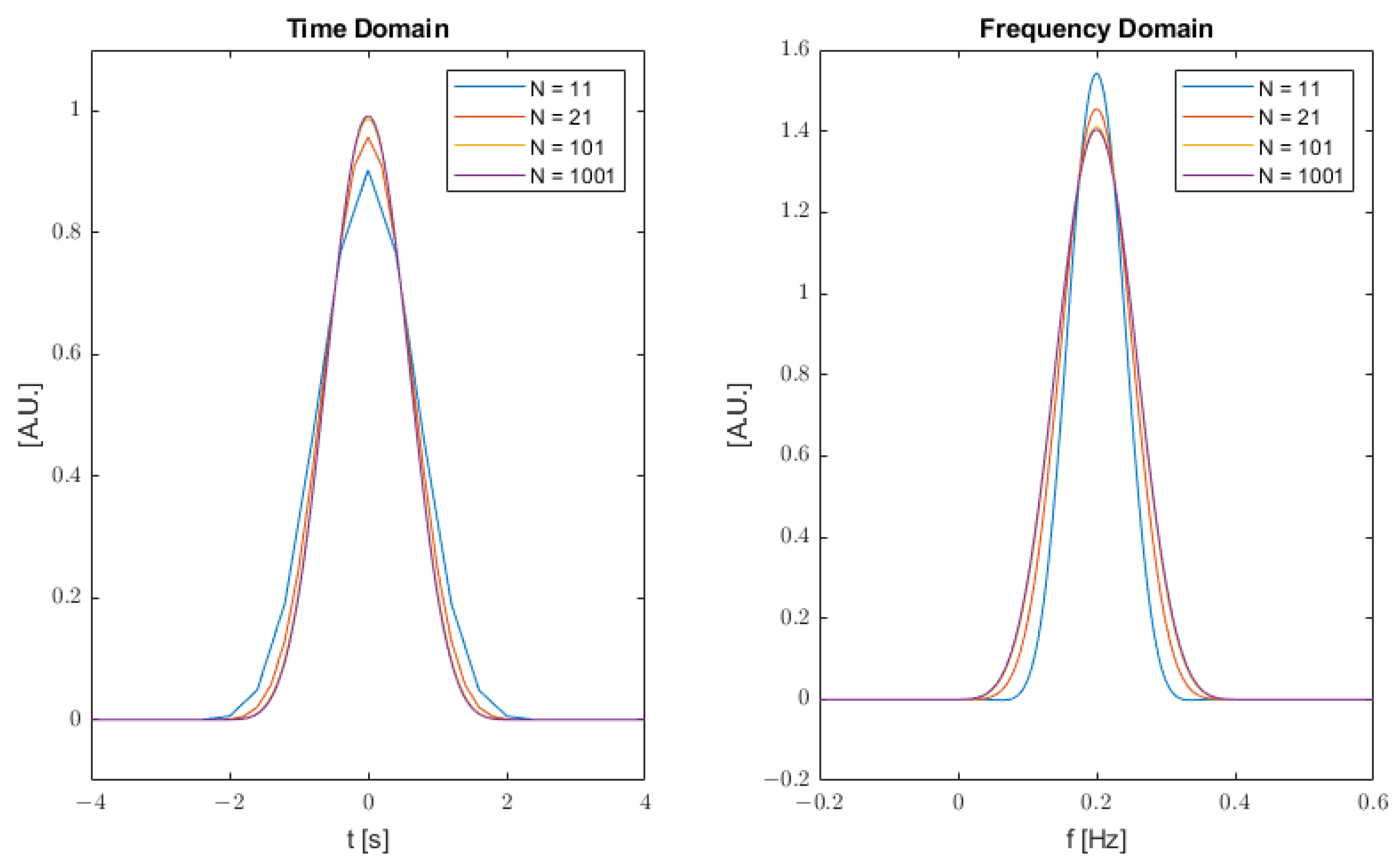
3.1. Mapping to Time Domain

Figure 1 shows four different zeroth order eigenvectors of Slepian bases with the same defining time bandwidth product $c=4$ but with different number of points (N).

Applying the mapping method presented in Section 2, the zeroth order eigenvector of the Slepian bases with different number of points (Figure 1) are mapped to the time domain to become discrete-time vectors. Time and frequency domain plots are shown for various choices of N in Figure 2. In Figure 2, all the Slepian zeroth order eigenvectors are specified with the time variable corresponding to $T_S=2s$, that is, they are defined on $\left[-T_S,T_S\right]$. The frequency domain plots show that the Slepian bases are concentrated inside the bandwidth $\left[-B_S,B_S\right]$ where $B_S=\frac{c}{2T_S}$. Here, $B_S=1$ Hz.

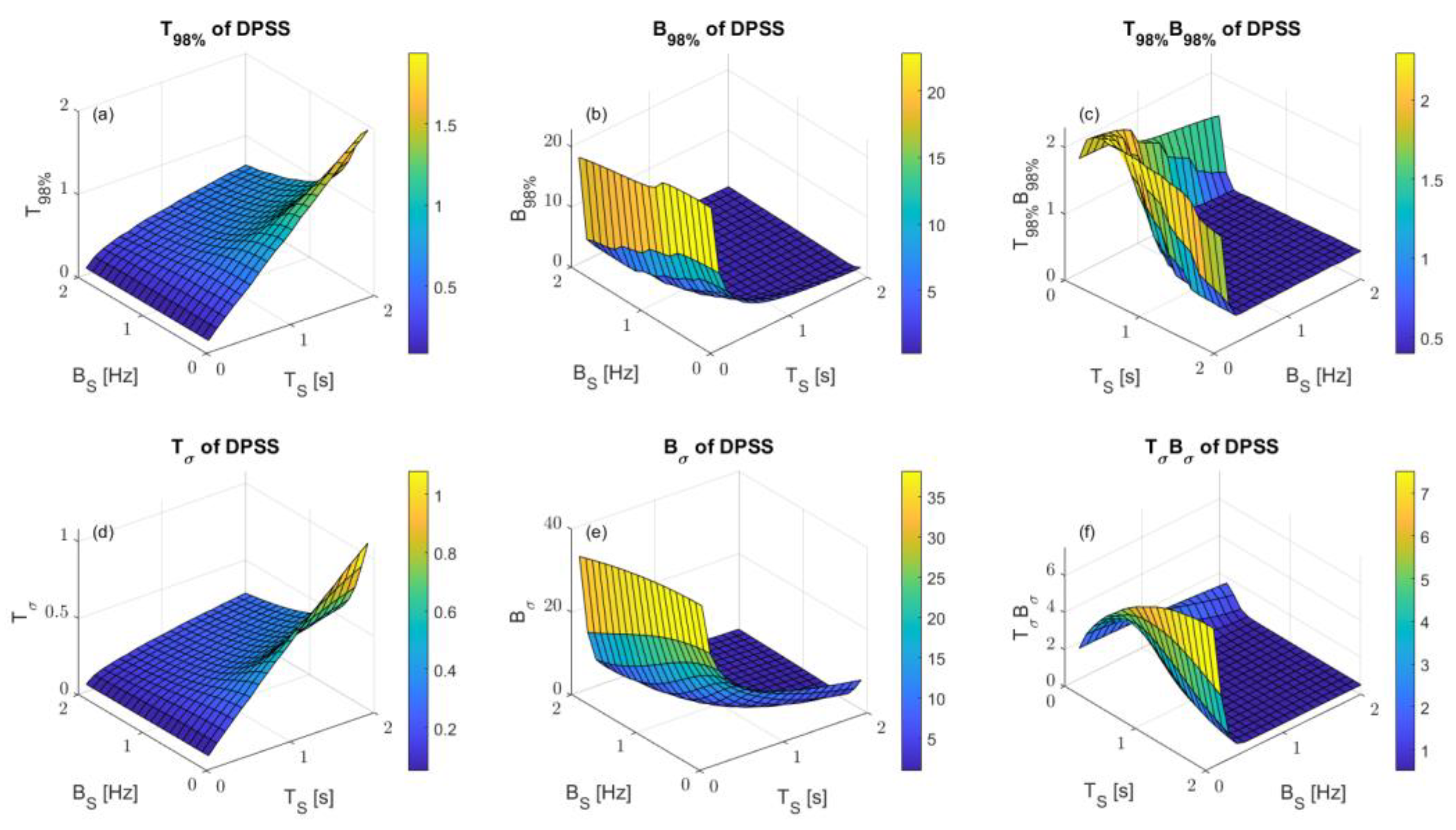
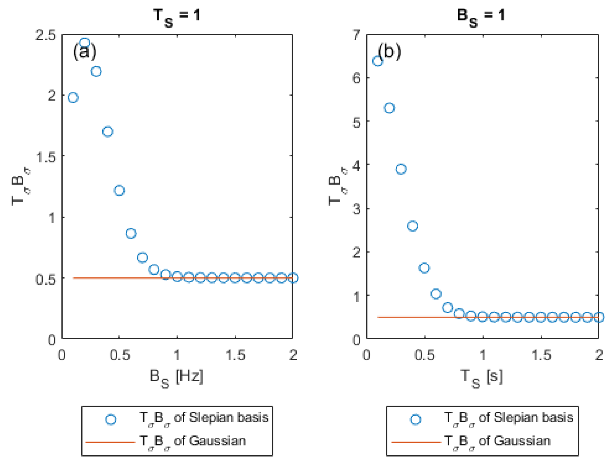
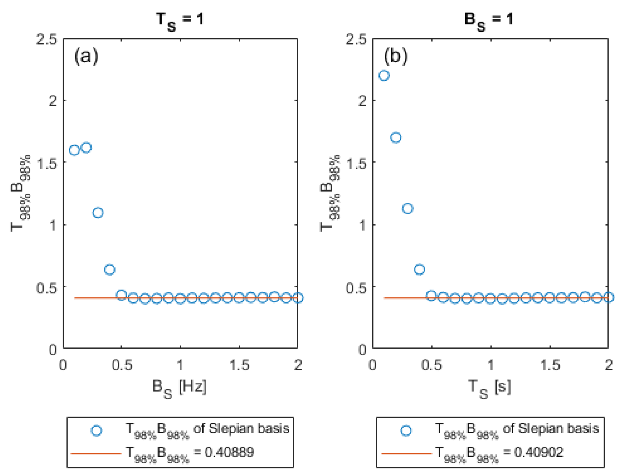
3.2. Time Frequency Characteristics

Figure 3 shows the effect of changing the defining duration and bandwidth on the effective duration and bandwidth (using both variance and energy definitions) of zeroth order Slepian eigenvectors. Time and frequency characteristics of 400 Slepian zeroth order eigenvectors are shown using the proposed method. The defining time and bandwidth of the Slepian bases ranged from 0.1 to 2 s (time parameter, so total duration 0.2–4 s) and 0.1 to 2 Hertz (bandwidth). Data from four hundred Slepians provide enough detail to visualize the trends. As can be seen from Figure 3, the two measurements of effective time bandwidth products $T_{\sigma }{B}_{\sigma }$ and $T_{98\%}{B}_{98\%}$ converge to a constant value when the defining time bandwidth products $T_S{B}_S$ of the Slepian zeroth order eigenvector increase. $T_S{B}_S$ are denoted as ‘defining’ time-bandwidth since they are used to generate the discrete vectors. However, the simulations show that although the Slepians are time(index)-limited in $T_S$ and band-concentrated in $B_S$ by definition, the effective time-bandwidth values $T_{\sigma }{B}_{\sigma }$ and $T_{98\%}{B}_{98\%}$ are not the same as the defining $T_S{B}_S$. As the Slepian defining-parameter time-bandwidth product ($T_S{B}_S$) increases, the actual effective time-bandwidth products (in the sense of variance or energy-based definitions) converge to constant values.

Figure 4a shows the (variance) effective time bandwidth products $T_{\sigma }{B}_{\sigma }$ of the Slepian zeroth order eigenvector with fixed $T_S=1\hspace{0.33em}s$ and varying $B_S$, and Figure 4b shows the (variance) effective time bandwidth products $T_{\sigma }{B}_{\sigma }$ Slepian basis with fixed $B_S=1\hspace{0.33em}\mathrm{Hz}$ and varying $T_S$.

Gaussian functions are known to have the smallest (variance definition) time bandwidth products $T_{\sigma }{B}_{\sigma }=0.5$, where this minimum possible time bandwidth product is governed by the (variance) uncertainty principle [9,14]. To enable the exploitation of symmetry of intervals and symmetry of Fourier definitions, we note that in our nomenclature for this paper, the T variable represents an interval of [−T,T] (i.e., the length of the interval is 2T).

From Figure 4, the (variance) effective time bandwidth products $T_{\sigma }{B}_{\sigma }$ for Slepian basis approaches this minimum limit of 0.5 when the defining $T_S{B}_S$ increases. Essentially, as the Slepian-defining time-bandwidth products increase, the defining constraints on time and bandwidth become less restrictive. This gradual ease in constraints allows the Slepians to approach the optimal compactness of the Gaussian functions, and the theoretical minimum time bandwidth product allowed by the uncertainty principle. This convergence towards the minimum effective time bandwidth product (variance definition) occurs at about $T_S{B}_S\approx 1$.

A similar trend can be observed with the 98% energy criteria of time and bandwidth definition, Figure 5.

As shown in Figure 5, as the defining time bandwidth product $T_S{B}_S$ increases, the effective time bandwidth product of Slepian zeroth order eigenvectors calculated with 98% energy criteria, $T_{98\%}{B}_{98\%}$, approaches the lower bound of ~0.4. Here, there is no significance to the value of 0.4 since choosing another percentage (e.g., 99% instead of 98%) in the energy-based definition will change the value of the lower bound. However, unlike the variance definition of compactness and the optimality of the Gaussians, there is no known function that satisfies the theoretical lower limit for the time bandwidth product when using the 98% energy criteria. The convergence towards the minimum energy-based effective time bandwidth product occurs at about $T_S{B}_S\approx 0.5$.

The classical (Fourier) uncertainty principle states that if a function is essentially zero outside an interval of length $\Delta t$ and its Fourier transform is essentially zero outside an interval $\Delta \Omega$, then $\Delta t\Delta \Omega \ge 1$ [14]. In our notation, this reads as $2T_{\%X}2B_{\%X}\ge 1$ or $T_{\%X}{B}_{\%X}\ge 0.25$. We have shown that the $\Delta t$ and $\Delta \Omega$ are not necessarily equal to the ‘expected’ Slepian-defining values of $2T_S$ and $2B_S$, in particular for small values of $T_S{B}_S$. Changing the choice of definition of ‘essentially zero’ affects the defining $T_S{B}_S$ for which the minimum lower bound is first reached. For example, if we were to choose ‘essentially zero’ defined through the variance definition, the defining $T_S{B}_S$ for which the minimum lower bound is reached is different, as demonstrated above. In applications, it may be desired to choose the smallest $T_S{B}_S$ for which minimum compactness is reached. Using the energy-based effective time-bandwidth definition for compactness, the smallest defining $T_S{B}_S$ to reach minimum compactness is $T_S{B}_S=0.5$. Slepians with values of $T_S{B}_S$ smaller than 0.5 will not reach minimum compactness. Instead, $\Delta t_{eff}\Delta {\Omega }_{eff}>1$ (strictly greater than 1) will be satisfied. That is, Slepians with values of $T_S{B}_S$ smaller than 0.5 tend to spread. Slepians with values of $T_S{B}_S$ larger than 0.5 will achieve minimum compactness but at the expense of a larger defining $T_S{B}_S$, which may or may not satisfy other constraints given in the application problem.

4. Conclusions

This paper proposed a method of mapping the index limited zeroth order Slepian basis to a discrete-time vector. This allows it to be used as a discrete function of time, which can be convenient for use in engineering applications. The time bandwidth concentration properties of the Slepian zeroth order eigenvectors are discussed. Results show that when the defining time bandwidth product $T_S{B}_S$ increases, the effective time bandwidth products calculated with variance $\left(T_{\sigma }{B}_{\sigma }\right)$, and 98% energy criterion $\left(T_{98\%}{B}_{98\%}\right)$ definitions converge to minimum values. This result agrees with known uncertainty principles for minimum time-bandwidth products. This indicates that not only are the zeroth order Slepian bases known to be optimally time-limited and band-concentrated basis vectors, but as their defining time-bandwidth products increase, their effective time-bandwidth properties approach known minimum compactness limits allowed by uncertainty principles. Furthermore, using the percentage energy definition of compactness allows us to conclude that the smallest value of Slepian defining time-bandwidth product to meet the minimum allowable compactness of the classical Fourier uncertainty principle is given by $T_S{B}_S\approx 0.5$. This conclusion gives guidance for applications where the time-bandwidth product is free to be selected and hence may be selected to achieve minimum compactness.

References

1. Hague, D.A. Adaptive Transmit Waveform Design Using Multitone Sinusoidal Frequency Modulation. IEEE Trans. Aerosp. Electron. Syst. 2021, 57, 1274–1287. [Google Scholar] [CrossRef]
2. Lo Conte, L.R.; Merletti, R.; Sandri, G.V. Hermite Expansions of Compact Support Waveforms: Applications to Myoelectric Signals. IEEE Trans. Biomed. Eng. 1994, 41, 1147–1159. [Google Scholar] [CrossRef] [PubMed]
3. Cheng, S.; Wang, W.-Q.; Shao, H. Large Time-Bandwidth Product OFDM Chirp Waveform Diversity Using for MIMO Radar. Multidimens. Syst. Signal Process. 2016, 27, 145–158. [Google Scholar] [CrossRef]
4. Moazzeni, T.; Al Hasani, S.A.; Memon, M.I.; Hussaini, S.J. On the Effect of Compactness of Pulse Shaping Function on Inter-Symbol Interference. IEEE Commun. Lett. 2022, 26, 828–832. [Google Scholar] [CrossRef]
5. Parhizkar, R.; Barbotin, Y.; Vetterli, M. Sequences with Minimal Time–Frequency Uncertainty. Appl. Comput. Harmon. Anal. 2015, 38, 452–468. [Google Scholar] [CrossRef]
6. Rihaczek, A. Signal Energy Distribution in Time and Frequency. IEEE Trans. Inf. Theory 1968, 14, 369–374. [Google Scholar] [CrossRef]
7. Baddour, N.; Sun, Z. Photoacoustics Waveform Design for Optimal Signal to Noise Ratio. Symmetry 2022, 14, 2233. [Google Scholar] [CrossRef]
8. Slepian, D.; Pollak, H.O. Prolate Spheroidal Wave Functions, Fourier analysis and Uncertainty—I. Bell Syst. Tech. J. 1961, 40, 43–63. [Google Scholar] [CrossRef]
9. Landau, H.J.; Pollak, H.O. Prolate Spheroidal Wave Functions, Fourier analysis and Uncertainty—II. Bell Syst. Tech. J. 1961, 40, 65–84. [Google Scholar] [CrossRef]
10. Landau, H.J.; Pollak, H.O. Prolate Spheroidal Wave Functions, Fourier analysis and Uncertainty—III: The Dimension of the Space of Essentially Time- and Band-Limited Signals. Bell Syst. Tech. J. 1962, 41, 1295–1336. [Google Scholar] [CrossRef]
11. Slepian, D. Prolate Spheroidal Wave Functions, Fourier analysis and Uncertainty—IV: Extensions to Many Dimensions; Generalized Prolate Spheroidal Functions. Bell Syst. Tech. J. 1964, 43, 3009–3057. [Google Scholar] [CrossRef]
12. Slepian, D. Prolate Spheroidal Wave Functions, Fourier analysis, and Uncertainty—V: The Discrete Case. Bell Syst. Tech. J. 1978, 57, 1371–1430. [Google Scholar] [CrossRef]
13. Karnik, S.; Romberg, J.; Davenport, M.A. Improved Bounds for the Eigenvalues of Prolate Spheroidal Wave Functions and Discrete Prolate Spheroidal Sequences. Appl. Comput. Harmon. Anal. 2021, 55, 97–128. [Google Scholar] [CrossRef]
14. Donoho, D.L.; Stark, P.B. Uncertainty Principles and Signal Recovery. SIAM J. Appl. Math. 1989, 49, 906–931. [Google Scholar] [CrossRef] [Green Version]
15. Varah, J.M. The Prolate Matrix. Linear Algebra Its Appl. 1993, 187, 269–278. [Google Scholar] [CrossRef] [Green Version]
16. Breitenberger, E. SSA Matlab Implementation; 1995. [Google Scholar]
17. Singh, N.; Pradhan, P.M. Achievable Simultaneous Time and Frequency Domain Energy Concentration for Finite Length Sequences. IET Signal Process. 2019, 13, 736–746. [Google Scholar] [CrossRef]
Figure 1. Zeroth order Slepian basis vector with time bandwidth product with c = 4.
Computation 11 00116 g001
Figure 2. Time and frequency plots of Slepian zeroth order eigenvectors with c = 4.
Computation 11 00116 g002
Figure 3. Time and Bandwidth measurements of Slepian basis (a) Change of effective time T 98 % with respect to defining time T S and bandwidth B S ; (b) Change of effective bandwidth B 98 % with respect to defining time T S and bandwidth B S ; (c) Change of effective time bandwidth product T 98 % B 98 % with respect to defining time T S and bandwidth B S ; (d) Change of effective time T σ with respect to defining time T S and bandwidth B S ; (e) Change of effective bandwidth B σ with respect to defining time T S and bandwidth B S ; (f) Change of effective time bandwidth product T σ B σ with respect to defining time T S and bandwidth B S .
Computation 11 00116 g003
Figure 4. (Variance) effective time bandwidth products (variance definition) of Slepian basis (a) TS = 1 s and varying BS and (b) BS = 1 Hz and varying TS.
Computation 11 00116 g004
Figure 5. (Energy-based) effective time bandwidth products (98% energy definition) of Slepian basis (a) TS = 1 s and varying BS and (b) BS = 1 Hz and varying TS.
Computation 11 00116 g005
Disclaimer/Publisher’s Note: The statements, opinions and data contained in all publications are solely those of the individual author(s) and contributor(s) and not of MDPI and/or the editor(s). MDPI and/or the editor(s) disclaim responsibility for any injury to people or property resulting from any ideas, methods, instructions or products referred to in the content.