1. Introduction
Filling gaps in observed time series is an important problem in many areas of applied sciences that depend on data analysis. Without this filling, data reconstruction is difficult or even impossible. This assumption is particularly true in weather forecasting, where the amount of stored information is growing four times faster than the world economy [
1]. In view of this, big data analytics can help to improve predictions by uncovering patterns and correlations in the data [
2] and reconstructing missing data in areas where there is limited information. Conversely, this growth in data also means that the amount of missing data is increasing, which makes accurate reconstruction a crucial task. To handle this challenge, forecasting methods must be able to handle large amounts of data, multiple data sources and a wide variety of meteorological variables. This requires advanced methodologies that can adapt to the particular characteristics of big data in weather forecasting.
Despite the general abundance of weather data available, there are still many regions without historical data records. These locations, which may be remote or under-developed, have the potential to be significant generators of renewable energy. However, without historical weather data, it is difficult to accurately predict the potential for energy generation in such places. Therefore, there is a growing need for methods that can generate weather data from limited inputs and locations, with the purpose of running simulations of environmentally driven systems that target these locations. This may greatly enhance our understanding of the potential for renewable energy generation, and may facilitate the development of sustainable energy systems in such regions [
3].
The field of weather prediction is often faced with two considerable challenges: (i) missing or absent weather data, and (ii) handling large volumes of data. The first challenge can be addressed through weather data reconstruction techniques known as hindcasting. Hindcasting enables the reconstruction of missing historical data (non-recorded observations) through the use of a generic prediction model to recreate past weather conditions. For this reason, hindcasting is also used for the validation of forecast models by comparing their output to past observations.
Besides the reconstruction of missing data, research in the field of hindcasting also aims to improve various aspects of meteorology, such as downscaling and forecasting methods. One of the key techniques employed in meteorological data reconstruction is the Analog Ensemble (AnEn) method [
4,
5]. Although the original AnEn method was first proposed for postprocessing Numerical Weather Predictions (NWPs), this technique has been applied in several areas, as the production of renewable energies (wind and solar) [
6,
7].
Overcoming the challenge of handling large volumes of data is essentially based on improving the efficiency of the numerical and computational methods employed. In the context of hindcasting, one possible approach is to use data reduction techniques. Another strategy involves improving the algorithms and their implementations. For instance, the employment of clustering techniques (as recommended by [
8]), which implies previously grouping the analogs data records, reduces the number of operations needed to identify the analogs and compute the reconstructed value (c.f. [
9,
10]).
The AnEn method combined with K-means clustering (ClustAnEn) has been successfully implemented in the reconstruction of missing gaps in time series by means of the values of one or two predictor time-series of correlated meteorological variables [
9,
11,
12]. In the study [
11], the clustering of analogs with the K-means was compared with other metrics used to determine the analogs, showing that this method performs better in terms of reconstruction accuracy. In another work [
13], it was also verified that the ClustAnEn combined approach is considerably faster than the classic AnEn method. Nevertheless, the reconstruction with more than two predictor time series of meteorological variables was not explored, mainly because it greatly increases the computational costs of clustering all possible analogs and does not benefit the results’ accuracy.
The difficulty in using a large number of predictors is not only relevant in the domain of hindcasting. It also exists in the field of forecasting, meaning that, until now, the number of predictors used has been relatively small, not exceeding five [
7,
14]. As will be shown in this paper, this difficulty can be overcome via dimension reduction techniques, in order to reduce the dimension of the original dataset without loss of essential information.
In view of the factors discussed above, it is clear that the AnEn method is highly promising for addressing challenges in hindcasting, forecasting and downscaling. To provide further evidence, a number of studies have also been conducted to compare the effectiveness of AnEn with other methods, namely convolutional neural networks (CNNs). For example, studies such as [
15,
16] have found that the AnEn method can improve prediction accuracy equally or even outperform CNNs when used to post-process results of regional weather prediction models, such as the Weather Research and Forecasting (WRF). Furthermore, the implementation of the AnEn method is relatively straightforward, and its results are easy to understand and explain, when compared to machine learning methods [
17]. These findings provide a strong basis for the continued use of the AnEn methodology in future research in the field of weather prediction and reconstruction.
In this study, we enrich the AnEn method with techniques that take advantage of a high number of predictor variables through dimension reduction. We explore the reduction in the original predictor dataset to a small number of new predictor variables, without loss of essential information. This original approach improves the quality of the reconstructions as well as their computational efficiency. We explore the dimension reduction through two alternative methods, namely principal component analysis (PCA) and partial least squares (PLSs).
The PCA technique identifies the dimensions along which the data are most dispersed, i.e., that have the largest variance (see for instance [
18]). In this way, we can identify the dimensions that best differentiate the dataset under analysis, i.e., its principal components that, in turn, are used as the new predictor variables. The PLS technique extracts from the set of predictor variables a set of latent (not directly observed or measured) variables which have the best predictive power. These new predictor variables are obtained by maximizing the covariance between the predictors and the predicted variable (see for instance [
19]).
In this work, we combine the AnEn method with PCA (PCAnEn) and PLS (PLSAnEn), in order to take advantage of the potentialities of the AnEn method and the dimension reduction provided by the PCA and PLS techniques. Furthermore, PCA and PLS are usually combined with multivariate linear regression, giving rise to the principal components regression (PCR) and partial least square regression (PLSR) methods. We present a comparative study of the performance of all these methods in a hindcasting problem, corresponding to the reconstruction of missing data in a given meteorological station by means of data coming from a set of predictor stations with different geographical locations.
The remaining of the paper is organized as follows.
Section 2 presents the various reconstruction methods employed in this study.
Section 3 introduces the meteorological datasets used.
Section 4 and
Section 5 focus on the selection of principal components and latent variables, respectively. In
Section 6, the numerical results of the tests performed with the various reconstruction methods are presented.
Section 7 provides an analysis of the computational performance of the same methods. Finally,
Section 8 concludes the paper, summarizing the main findings and their implications for the solving of hindcasting and forecasting problems with a high number of predictors.
2. Reconstruction Methods
This section briefly describes all the reconstruction methods used in this work. It begins by presenting the analog ensemble method, which is the foundation for the other hindcasting methods. This is followed by an introduction to dimension reduction methods, using PCA and PLS, and their use to reconstruct missing values.
2.1. Analog Ensemble Method
In this work, the AnEn method is used to reconstruct meteorological records missing in a time series. Reconstruction of missing values in a time series is a problem equivalent to hindcasting, i.e., to predict past events recurring to a forecast method and historical data (e.g., measurements at some other location or from another variable). The data are reconstructed based on one or more predictor time-series that present some type of correlation with the incomplete series to be reconstructed/predicted.
A practical application scenario consists of reconstructing data from a meteorological station using data from neighboring stations. In this context, several time-series are used as predictors, being represented by the column vectors
each one containing
n records of the values of certain meteorological variables. For simplicity, these vectors will often be referred to as predictor variables.
The predictor variables can be used in a
dependent or
independent way. In the dependent variant, the analogs selected in different predictor variables must be concomitant (overlapping) in time. In the independent version, such is not mandatory. In previous work [
11], it was verified that the dependent version of the AnEn method is more accurate and therefore, from now on, that is the version assumed to be used, unless otherwise stated.
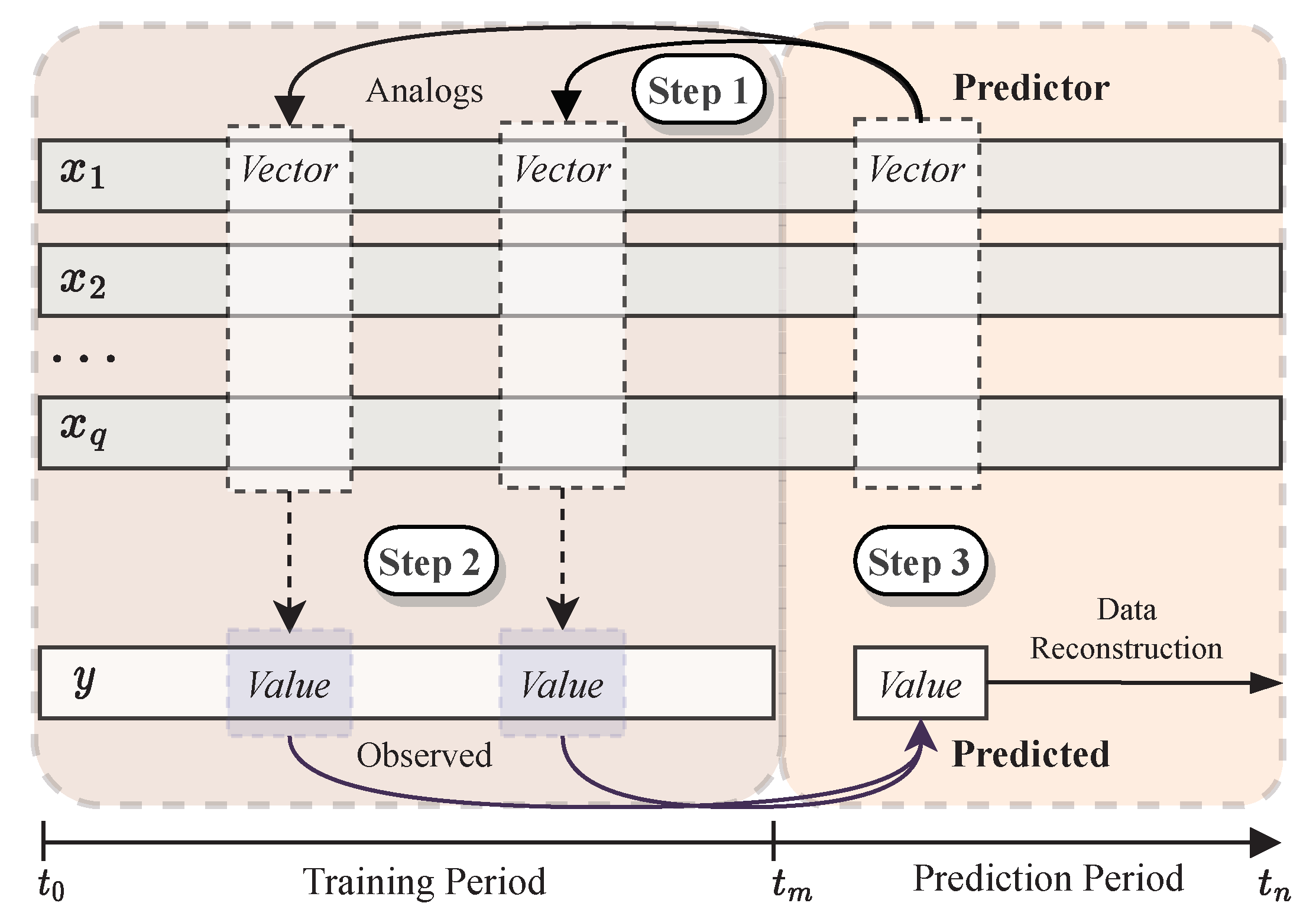
In
Figure 1, the AnEn method is illustrated with
q predictor variables. The historical data is complete in the predictor variables and incomplete in the reconstructed/predicted one (
). The period of missing records is denoted as the
reconstruction period, but, often, it is also designated as
prediction period. This designation originates from the application of the AnEn method to the post-processing of meteorological forecasts, in which the predictor series contains the history of forecasts. In this work, the reconstruction period corresponds to the part of the time-series in which the records are reconstructed (or, by analogy, predicted). The period for which all series contain full data is known as the training period. The longer the training period (compared to the prediction period), the better the AnEn method is expected to perform (the more comparison data, the more likely it will be to find meteorological conditions similar to those sought).
As depicted in
Figure 1, firstly (step 1), a certain number of analogs are selected in the training period of the predictor variables, due to being the past records most similar to the predictor record at instant
. To evaluate the analogs, a time window is defined that encompasses the predictor record at time
and its
k consecutive neighbors in the recent past (
,
, ...,
) and immediate future (
,
, ...,
); these
records make up a predictor vector. Next, the same kind of time window is defined for each and every instant in the training period,
, with a corresponding training vector; the comparison of all the training vectors with the predictor vector makes it possible to assess their similarity (see [
11] for similarity metrics); the training vectors most similar to the predictor vector form the analog ensemble. Note that comparing vectors, instead of single values, accounts for the evolutionary trend of the meteorological variable around the central instant of the time window, allowing for the selection of analogs to take into consideration weather patterns (instead of single isolated values). A range of
was reported to enhance prediction accuracy [
12]; thus, this study employed
to reduce computational demands while still attaining optimized predictions. For the datasets under analysis in this work, the resulting time window corresponded to one hour, as the time series had a sampling period of 6 minutes.
In step 2, the analogs are mapped onto observations of the predicted station, by selecting the simultaneous records in the observed time-series. This mapping is conducted only for the central time of each analog time window, i.e., for each analog vector a single observed value is selected in the training period.
Finally, in step 3, the observed values chosen are used to predict (reconstruct) the missing values in the predicted variable , through its average (weighted or not). When this target value is actually available as real observational data (as it happens in this work), it becomes possible to compute the error of the reconstruction/prediction and, consequently, to validate the method.
2.2. ClustAnEn Method
The extension of the training period has an influence in the performance of the AnEn method. The longer the training period, the more accurate the predictions/reconstructions are expected to be. On the other hand, longer training periods imply greater computational effort to identify the analogs in each reconstruction. To alleviate this problem, an alternative version of the AnEn method was developed in which all possible analogs (all of the time windows that one can make from the predictor variables in the training period) are previously classified into a predefined number of clusters [
9,
13], with the number of clusters set to the square root of the total number of possible analogs. This heuristic is based in the empirical results previously obtained [
12]. In this way, a predictor vector is compared only with the centroid (median of the analogs in that cluster) of each cluster in order to identify the
analog cluster that contains the analogs selected in step 1. This AnEn variant, denoted ClustAnEn, is much faster than the classic AnEn method in identifying the analog ensemble [
13].
Another important issue in data reconstruction/prediction is the number of predictor variables. It is expected that the more predictors there are, the more useful information for the reconstruction is available. Hence, it is important to know how reconstruction/prediction methods can use all available predictive information. As the AnEn and ClustAnEn methods lose computational efficiency with the increase in the number of predictor variables, the use of these methods is not suited for a large number (q) of predictor variables. Therefore, the main objective of this work is to reduce the dimension of the predictor dataset, while minimizing the loss of information, in order to be able to use the AnEn and ClustAnEn methods in hindcasting and forecasting problems with a high number of predictor variables.
2.3. Principal Components Analysis
The Principal Components Analysis (PCA) technique makes it possible to reduce the dimensionality of a dataset consisting of a large number of interrelated variables, while retaining as much of the information of variation present in the dataset as possible. This is achieved by transforming to a new set of uncorrelated variables, called the principal components (PCs), which are ordered so that the first few contain most of the variation information present in original variables dataset [
18]. We describe here, briefly, the application of PCA to the dimension reduction in predictor variables.
Let the original dataset of predictor variables be represented by the matrix
where predictor variables are represented by the
q column vectors
, with
, each one with
n records of the value of a given meteorological variable. The matrix
is assumed to be centered, i.e., the mean of each column is equal to zero, and standardized such that its variance equals unity. To identify the dimensions along which the data are most dispersed, i.e., the dimensions that best differentiate the predictor dataset, it is necessary to compute the principal component (PC) vectors. Such can be achieved by the thin singular value decomposition of the predictor matrix
, given by
where the columns of the matrix
contain the left singular vectors, the diagonal matrix
contains the singular values
, with
and the matrix
contains the right singular vectors
, with
, which are the
principal components directions of
(for details see [
20]). The matrices of the left and right singular vectors are orthonormal, i.e.,
, where
is the identity matrix.
The vectors
are the principal components (PCs) of the original dataset and define new variables that will be used instead of the original predictor variables. The first principal component,
, has the largest sample variance, equal to
, among all normalized linear combinations of the columns of
[
20]. The second principal component, given by
, is the new variable with the second largest variance (
). Likewise, the remaining principal components define new variables with decreasing variances.
The new variables
are linear combinations of the columns of
, i.e., the original predictor variables
, being given by
where the coefficients
, with
, designated as
loadings, are the elements of the vector
. The magnitude of a coefficient is related to the relative importance of the corresponding original variable in the principal component.
The substitution criterion of the original predictor variables,
, by
p PCs,
, with
, in the AnEn or ClustAnEn methods, must take into account the influence of the new variables in the original dataset. This influence is directly proportional to the respective variances, which are given by
, with
. It is expected that the first few principal components, corresponding to the largest singular values, account for a large proportion of the total variance, being all that is needed do describe the original dataset [
21]. Therefore, one of the possible criteria that can be used to choose how many PCs should be used, is the magnitude of the respective singular values. If the original variables are previously scaled, by dividing each variable by the respective standard deviation, each of them will have a standard deviation equal to one. If a PC has a standard deviation greater than one, it means that it contains more information than any of the original variables and, as such, should be chosen to represent the original dataset.
In an exploratory study on the use of the AnEn method based on the principal components of a meteorological dataset [
22], it was verified that the efficiency of this combination strongly depends on the correlation between the predictor variables. If they are poorly correlated, it is not possible to reduce them to a small number of components without losing significant information. On the contrary, if the predictor variables are correlated, then it is possible to reduce their dimension to a small number of components and improve the quality of the prediction with the AnEn method.
The combination of the AnEn and ClustAnEn methods with PCA gives rise to two new methods that are designated in this work by PCAnEn and PCClustAnEn, respectively.
2.4. Principal Component Regression
As an alternative to the reduction in the size of the predictor dataset, the reconstruction of missing data can be accomplished using multivariate linear regression. This method, unlike the AnEn method, allows for the direct use of all the original predictor variables.
The goal of the multivariate regression is to predict
from
, where
contains in the columns the values of all the predictor variables recorded during the training period, and
the corresponding values of the predicted variable. This problem involves the determination of the vector
, that is, the approximated solution of the linear system of equations
Such is equivalent to solve the linear least squares problem
where
is the usual 2-norm (see [
20] for details). If
is a full rank column matrix, then the solution of the problem (
7) is given by
The expectation is that the solution vector
can be used to predict values in the reconstruction period based on the predictor variables for that same period, that is:
where
represents the reconstructed/predicted variable during the reconstruction/prediction period and
contain the values of the predictor variables along the same period.
The multivariate regression model given by Equation (
9) can be implemented only if the matrix
has full column rank (its column vectors are linearly independent). The near-collinearity of columns can occur if there are highly correlated predictor variables. In this case, the least squares problem (
7) becomes ill-conditioned and difficult to solve.
The principal component regression (PCR) [
23] method circumvents the rank deficiency by replacing the original predictor variables
by its principal components (PCs) in the regression model. Once the principal components,
, are obtained from matrix
in the same way as described in
Section 2.3, a few of them (
p) are used in the regression model to estimate
.
Therefore, the PCR method consists of regressing
not on
itself but on the principal components matrix
, assuming that
p PCs have been previously selected. This implies to solve by linear least squares the system
whose solution is the parameter vector
The PCR regression model on
is then given by
were
is, as before, the vector of the reconstructed/predicted values of
during the reconstruction/prediction period,
contains the values of the
p selected PCs along the reconstruction/prediction period and
is the parameter vector of the PCR.
The regression model (
12) can be expressed in function of
instead of
by replacing
by
, thus originating
PCR is an alternative to the AnEn-based methods that combines the size reduction provided by PCA with linear regression. This combination prevents collinearity problems between vectors of predictor variables. Another advantage of PCR is the reduction in the number q of original predictor variables to a lower number p of principal components, but which contain most of the original information. Thus, the good performance of this method depends strongly on the choice of the PCs.
It is expected that a few of the PCs, which have a higher variance, are enough to describe the evolution of the original predictor dataset. However, these components were chosen to explain the evolution of the original predictor variables, contained in the matrix and, as such, there is no guarantee that these PCs will be relevant for the prediction of .
2.5. Partial Least Squares Regression
In contrast with the PCR method, the partial least squares regression (PLSR) method uses the components from
that best predict
. These components, also called the latent variables (because they are not directly observed or measured), are coming from the joint decomposition of
and
, taking into account the obligation of the components to explain the covariance between
and
as best as possible [
24,
25].
PLSR computes the latent variables that model
and
and best predict
, resulting in the variable decompositions
where
and
are the matrix with
p latent vectors (also known as scores) extracted from
and
, respectively;
and
represent the loading vectors; the matrix
and vector
represent the residuals, whose norms are minimized. Additionally, the scores matrix
is orthogonal, that is,
. The decompositions (
14) can be achieved by different procedures, such as the nonlinear iterative partial least squares (NIPALSs) algorithm [
26] or the statistically inspired modification of PLS (SIMPLS) algorithm [
27].
The decompositions (
14) are performed in order to minimize the norm of the residual matrices,
and
, and to maximize the covariance between the latent vectors, columns of
and
. Consequentially, there is a linear relation between
and
, expressed as
where
is a diagonal matrix with the regression weights and
denotes the matrix of the residuals. Combining (
15) with the decomposition of
, given by (
14), leads to
or simply
where
denotes the regression vector and
is the residual vector, so that
can be estimated as
The regression model (
18) makes it possible to estimate
based on the latent variables
, but it is useful regressing
on the original predictor variables
. To accomplish this, the matrix
, of the PLS weights, computed such that
, is post-multiplied by the decomposition of
in (
14):
Replacing (
19) by (
18) returns an expression that can be applied to the training data:
where
is the parameter vector of the PLSR regression model. Since the solution of (
17) by linear least squares, with orthogonal latent predictors
, leads to
, the parameter vector (
21) can be written as
For the reconstruction/prediction period, the PLS regression model will be given by
where
is the matrix of the predictor variables along the reconstructions/prediction period and
represents the matrix of latent variables in the same period. Other formulations of the PLSR model can be derived based on the properties and identities between the vectors resulting from the algorithm used to obtain the decompositions (
14) (see, for instance, [
19,
25,
28]).
As Equation (
24) makes it possible to extend the latent variables along the prediction period (
), it is possible to use them as predictors in the AnEn-based method. In this work, we also explore the combination of the AnEn and ClustAnEn methods with the PLS decomposition, in order to use the latent variables as predictors instead of the original variables. The resulting methods are denoted PLSAnEn and PLSClustAnEn, respectively.
The PLS regression method is also, by itself, an alternative method to PCR and AnEn-based methods for the reconstruction/prediction of the missing records, by estimating them via the regression model (
23) and, therefore, is also included in the present study.
3. Meteorological Datasets
The US National Data Buoy Center (NDBC) [
29] is the source for the data used in this study. NDBC manages a network of coastal stations and buoys for data collection. Part of the National Oceanic and Atmospheric Administration (NOAA), the most representative weather center in America [
30], NDBC provides open-source, credible and updated data.
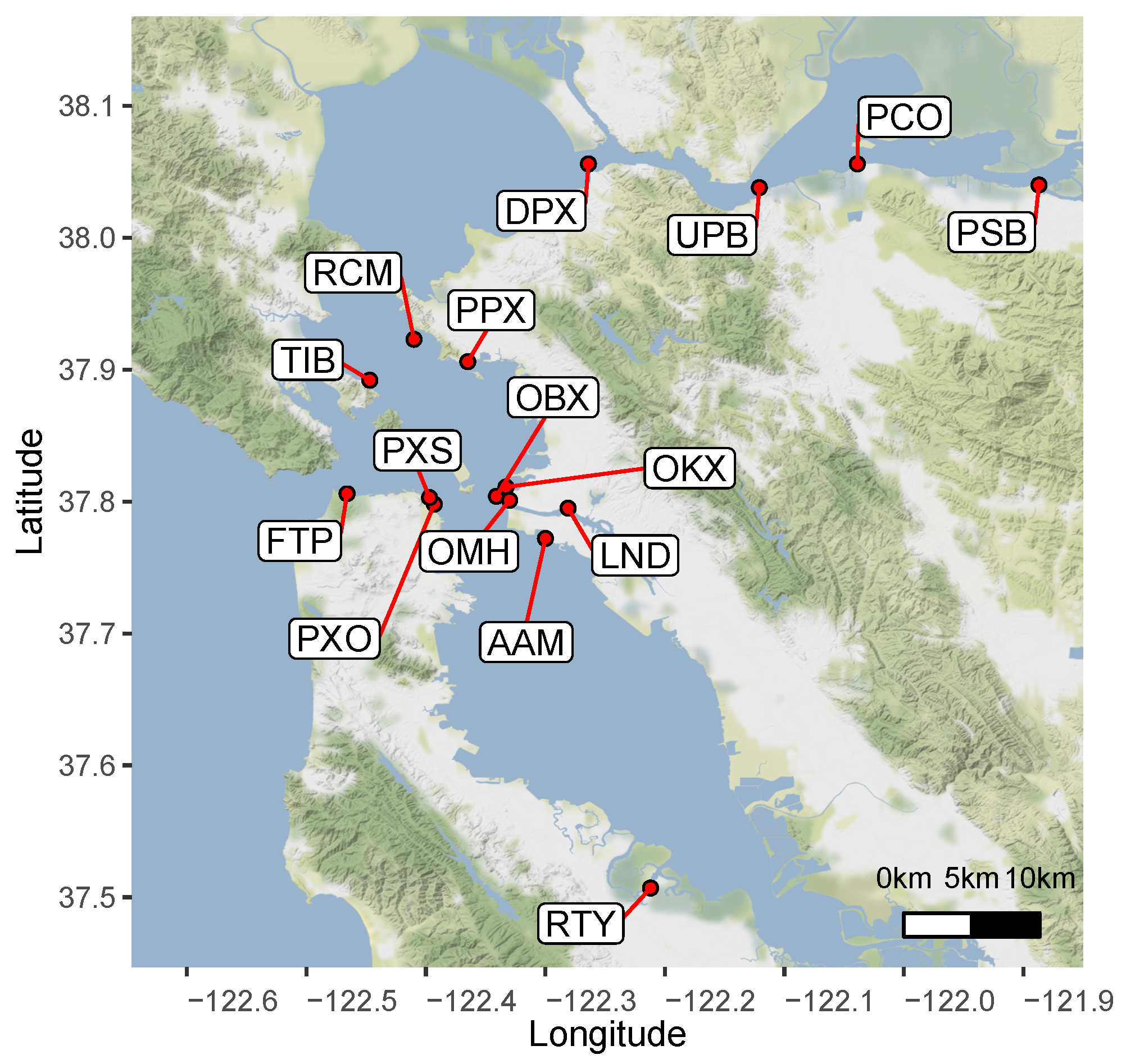
The NDBC database covers regions from almost the entire US coast, as well as some across the globe. For this work we focused on a region with a stations density as large as possible. The choice fell on a region centered on the north of the San Francisco Bay (California, USA), for which there are records produced by 16 meteorological stations relatively close to each other.
Figure 2 shows the selected region and its 16 NDBC stations.
Records of various meteorological variables are available for each station, with a sampling period of 6 min. The variables used in this study are atmospheric pressure (PRES) (mbar), air temperature (ATMP) (°C), wind speed (WSPD) (m/s) and peak gust speed (GST) (m/s). WSPD and GST can vary significantly over short time intervals, and sporadic data gathering incompletely describes their real behavior. NDBC solved this problem by sampling the wind speed (WSPD) every 6/8 s and averaging the readings across 6 min; additionally, it considers the maximum wind speed on the same interval as the peak gust speed (GST). In turn, the collection of ATMP and PRES is straightforward: the instantaneous value every 6 min is the one recorded in the NDBC database.
The records start in 1 January 2016 and end in 31 December 2021. Due to sensor failures and maintenance operations in the stations, variables often present time-series with incomplete data.
Table 1 presents the mean, standard deviation (SD) and availability (in percentage), for the considered variables (WSPD, GST, ATMP and PRES), in the 16 stations.
To maximize the amount of training data, only variables with more than 85% of availability (in bold in
Table 1) were chosen for this study. The presence of NA in
Table 1 means that the corresponding variable is not available at the corresponding station. Consequently, the working dataset consists of a total of 41 time series: 10 series with records of the WSPD variable, 10 of the GST variable, 12 of the ATMP variable and 9 of the PRES variable.
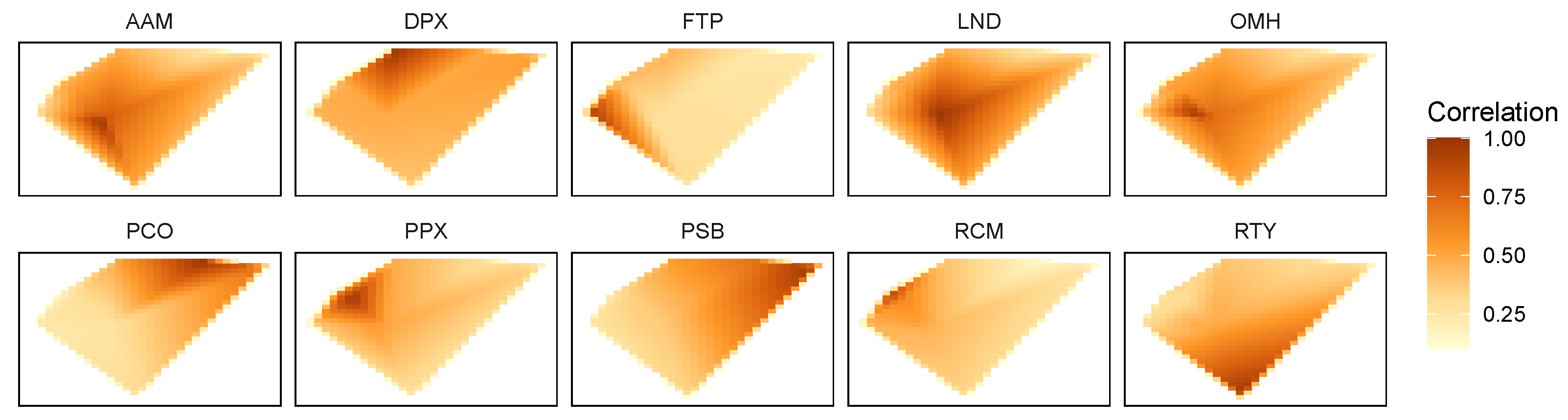
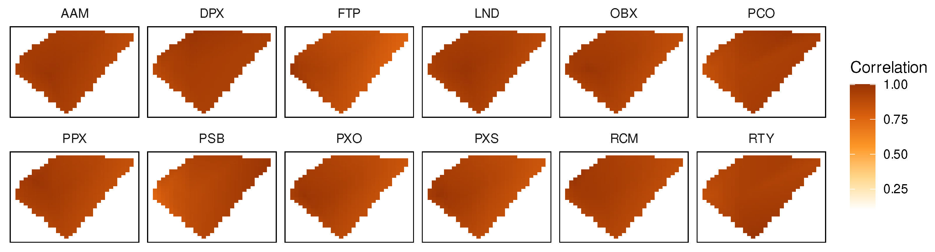
Figure 3,
Figure 4,
Figure 5 and
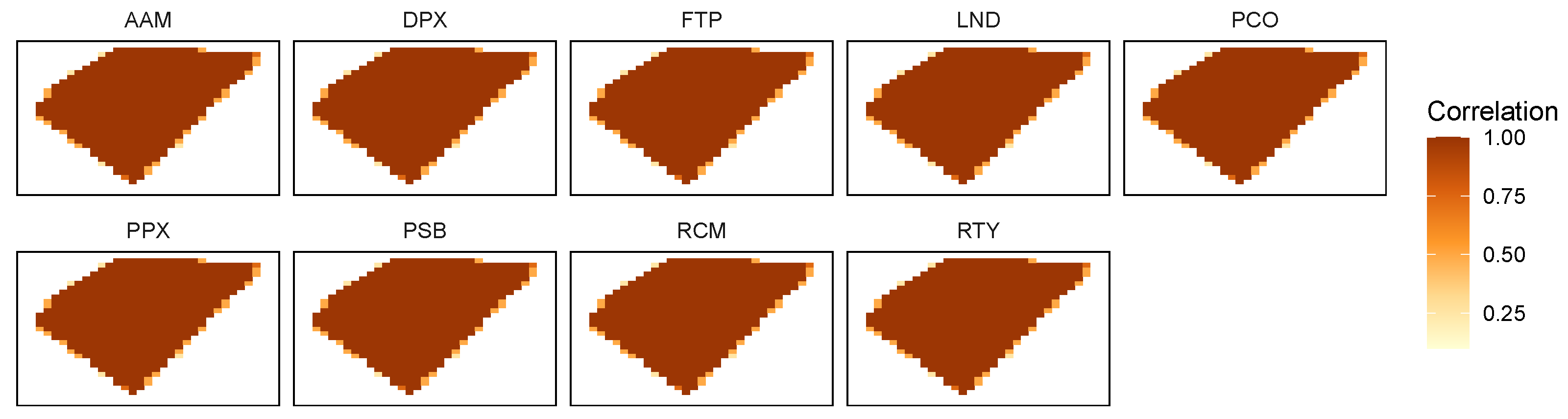
Figure 6 show the correlations between the stations with more records for each variable (10 stations for the WSPD, GST and ATPM variables, and 9 stations for the PRES variable). In each figure, a heat map is shown for each station; the polygonal format of this map matches (approximately) a four-side polygon that includes the 16 stations, preserving their geographical positions and distances, considering the layout of
Figure 2. In each heat map, only 10 (9) points represent station correlations—the points corresponding to their locations; the correlations for the other points were produced by interpolation.
As may be observed in
Figure 3 and
Figure 4, for the WSPD and GST variables only the closest stations present a strong correlation. Furthermore, the GST variable presents correlations between stations slightly higher than those observed for the WSPD variable. These observations confirm that the wind-dependent variables have a local (and not regional) variation, significantly depending on the morphology of the terrain where the station is implemented.
Figure 5 and
Figure 6 show that the ATMP and PRES variables have a different behavior from that of the WSPD and GST variables (
Figure 3 and
Figure 4), as ATMP and PRES present a very high correlation between stations, even among the most distant ones. This shows that the ATMP and PRES variables have a regional character, varying little or not at all locally.
4. Selecting the Principal Components
In this section, we show how the selection of the principal components (PCs) that are used in the PCAnEn, PCClustAnEn and PCR methods is conducted. The number of PCs to be included in these methods is of great importance. An insufficient number of PCs translates into the loss of information necessary for data reconstruction, whilst a high number translates into redundant information and increased computational costs.
The identification of the dimensions with most data dispersion makes it possible to identify the principal components
, with
, that best distinguish the dataset under study. The dataset corresponding to the multiple predictor time-series, from the various meteorological stations described in
Section 3, is represented by the data matrix
, where each column vector
, with
, includes the centered and scaled records of a single variable. The thin singular value decomposition of
makes it possible to obtain the principal components
,
, each one corresponding to a singular value
,
, where
(see
Section 2.3). The PC vector
has the largest sample variance (
),
has the second largest variance (
) and so on. On the other hand, as the original predictor time-series are previously scaled by the respective standard deviation, if a PC has a standard deviation greater than 1 it means that this PC defines a dimension with more dispersion, i.e., it contains more information than the original variables. This will be the criteria used to select the PCs, as employed in [
31].
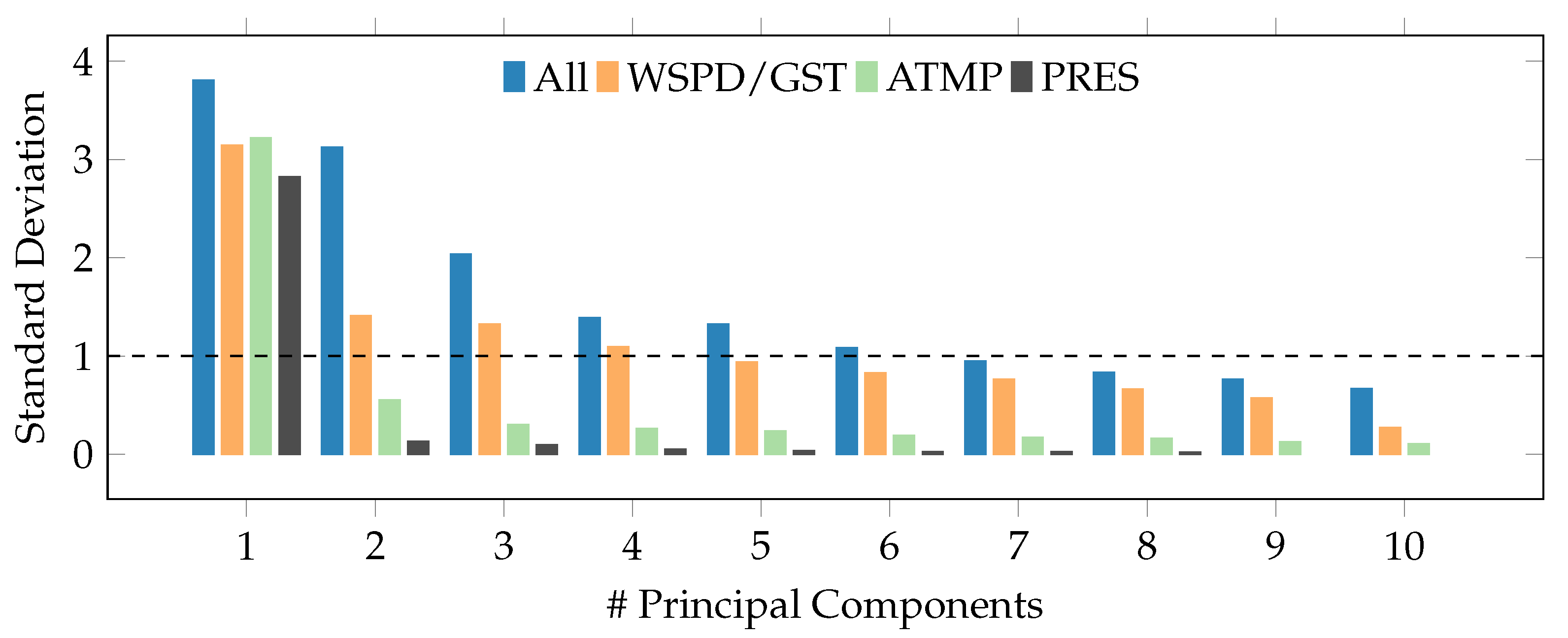
Figure 7 shows the standard deviations of the first 10 PCs obtained from 37 predictor variables of the dataset used. These predictor variables do not include the time-series from the PPX station because these series are used only as predicted/reconstructed variables.
Based on the same figure, the principal component analysis is performed from different predictor matrices
: in the first case (blue bars), the PCs are obtained from all predictor variables (
); in the second case (orange bars), the PCs are obtained by means of the predictor variables WSPD and GST (
); in the third case (green bars), only the ATMP time-series were used (
); finally, in the fourth case (gray bars), only the PRES series where considered as predictors (
). The idea behind this analysis is to verify whether there is any advantage in using predictor variables different from the predicted ones. Following [
22], the variables WSPD and GST were merged as they are highly correlated with each other; hence, it makes no sense to use them separately.
As can be seen in
Figure 7, where the PC choice threshold is indicated by a dashed horizontal line, if all variables are used as predictors then the first six PCs (
) must be selected to represent the predictor dataset. In the case of wind-related predictor variables (WSPD and GST), the first four PCs (
) must be used. Finally, for a single predictor variable (ATMP or PRES), only the first PC (
) should be chosen.
Table 2 shows the errors for the prediction/reconstruction of the variables WSPD, ATMP and PRES, of the PPX station, using the PCR, PCClustAnEn and PCAnEn methods, with the number of PCs previously defined (6, 4 or 1). The reconstruction period was the year of 2021 (the last one of the dataset) and the training period spanned from 2016 to 2020. Due to computing resource constraints, the daily records were reconstructed only from 10 am to 4 pm; moreover, the analogs were searched only in the same period. The reconstruction errors shown are the bias (BIAS), which is an indicator of the systematic error, the standard deviation of the error (SDE), an indicator of the random error and the root mean square error (RMSE), including both the systematic and the random error (for details see [
32]). The smallest errors are highlighted in bold.
As may be observed in
Table 2, with the exception of the ATMP variable, there seems to be no advantage in using all available predictor variables and, in most cases, it is preferable to use as predictor the same variable to be predicted/reconstructed. This is an indication according to which the proposed methods are not adequate to use all available information without scrutiny. Some signals (time-series) are uncorrelated with others and if these are used, they will introduce noise. Hence, the tests with limited variables, based on signals that share the same physical significance, have better results. Moreover, comparing the results obtained by the three methods, they result in errors very close to each other. At most, errors are in the order of tenths of a unit. Noteworthy, the consistent spatial correlation of ATMP and PRES, as seen in
Figure 5 and
Figure 6, gives PCRs a slight advantage in their reconstruction, which suggests that a regression model uses this correlation more effectively. In contrast, WSPD has lower spatial correlation and more frequent temporal variations, making PCAnEn the best method for its reconstruction. Finally, PCClusAnEn yields comparable or nearly identical results to PCAnEn, for all the three variables.
5. Selecting the Latent Variables
Choosing the number of components (latent variables) is an important step in the application of the PLSR method or variants. As a latent variable is relevant only if it improves the prediction of , it is firstly necessary to solve the problem of which and how many latent variables should be kept in the PLSR model to achieve optimal predictions.
In this section, we propose two approaches that can be used to determine the number of latent variables (p). To achieve this, the variables of the PPX station were predicted/reconstructed by means of the variables of the neighboring stations. Thus, there are original predictor variables that can be used to obtain latent variables.
The performance of a PLSR model can be evaluated with computer-based re-sampling techniques, such as cross-validation (c.f. [
33]). In this technique, the data of the training period (see
Figure 1) are split into a
learning set (used to build a PLSR model) and a
testing set (used to test the model). In particular, in the Leave-One-Out Cross-Validation (LOOCV) approach, the initial training dataset is partitioned into exactly
k subsets (
k-fold). Each subset is then used to test the PLSR model built by means of the data included in the
learning subsets (for details, refer to [
25,
34]). The predicted observations for each testing set are stored in the vector
, which is used to determine the overall quality of the PLSR model using
p latent variables. The quality of the PLSR model is evaluated by measuring the discrepancy between
and
, using the root mean-squared error predicted (RMSEP):
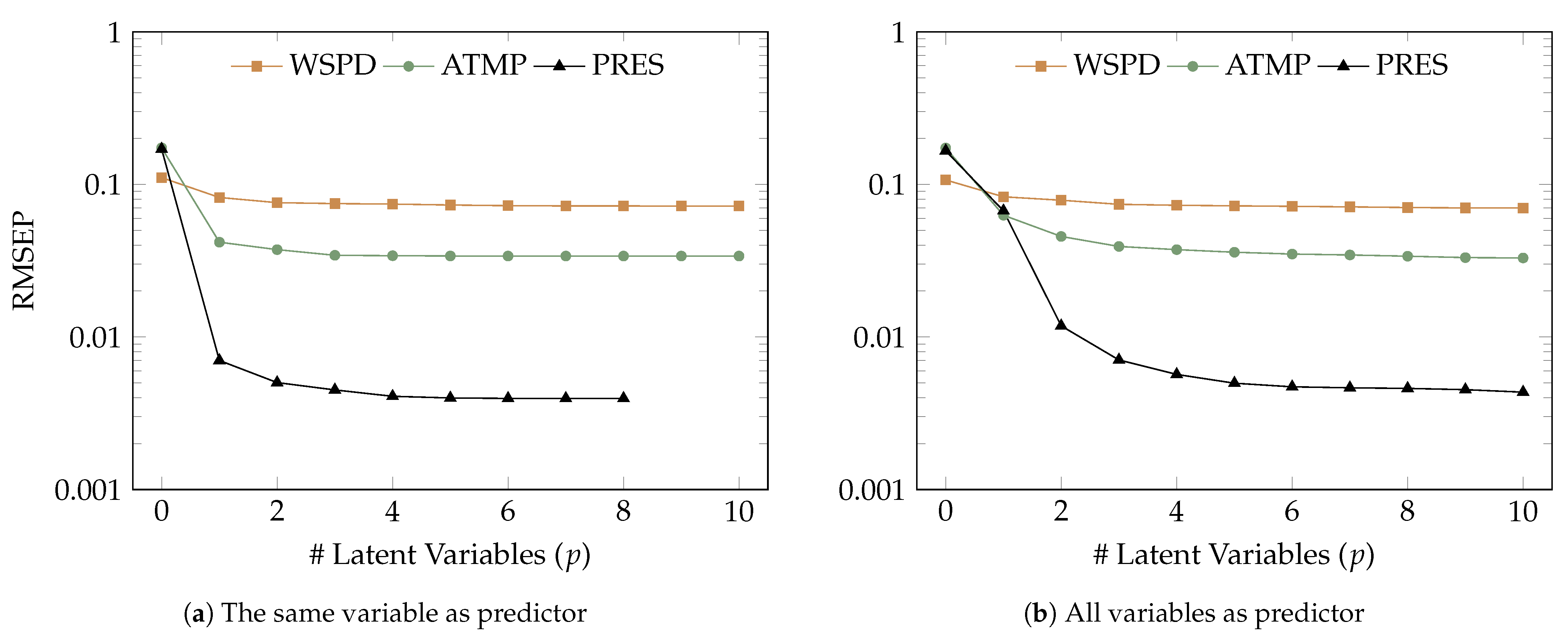
Figure 8a shows the values of the normalized RMSEP in function of the number of latent variables (
p), originated by the predictions of the four meteorological variables (WSPD, GST, ATMP and PRES), from the PPX stations, by means of the 10-fold LOOCV technique. Each variable was predicted only by the time-series corresponding to the same meteorological variable (
and
contain data from the same meteorological variable), except for WSPD and GST, which are used together to predict WSPD, based on the analysis in
Section 3. It can be observed, in the case of WSPD, that the first four components are responsible for the highest decrease in RMSEP. For a number of latent variables greater than four, the decrease in RMSEP is not significant. For the ATMP and PRES meteorological variables, the largest reduction in RMSEP happens for the first three components.
Figure 8b shows the values of the RMSEP generated in the same conditions as in
Figure 8a, with the exception that each variable was predicted by all meteorological variables in the neighboring stations. In the case of WSPD, the first two or three latent variables are responsible for the highest decrease in RMSEP. For the case of ATMP and PRES, the largest reduction in RMSEP occurs for the first three or four components.
An alternative approach to determine the optimal number of latent variables is based on the metric
where
is the predicted residual sum of squares originated by the LOOCV technique, with the
p latent variable, being computed through
and
is the residual sum of squares originated by the PLSR model, obtained with the
latent variable and built with all data from the training period. The idea of this criteria, proposed in [
36], is that a latent variable is kept if the value of the metric (
26) is larger than a certain threshold (
) generally set to
, i.e.,
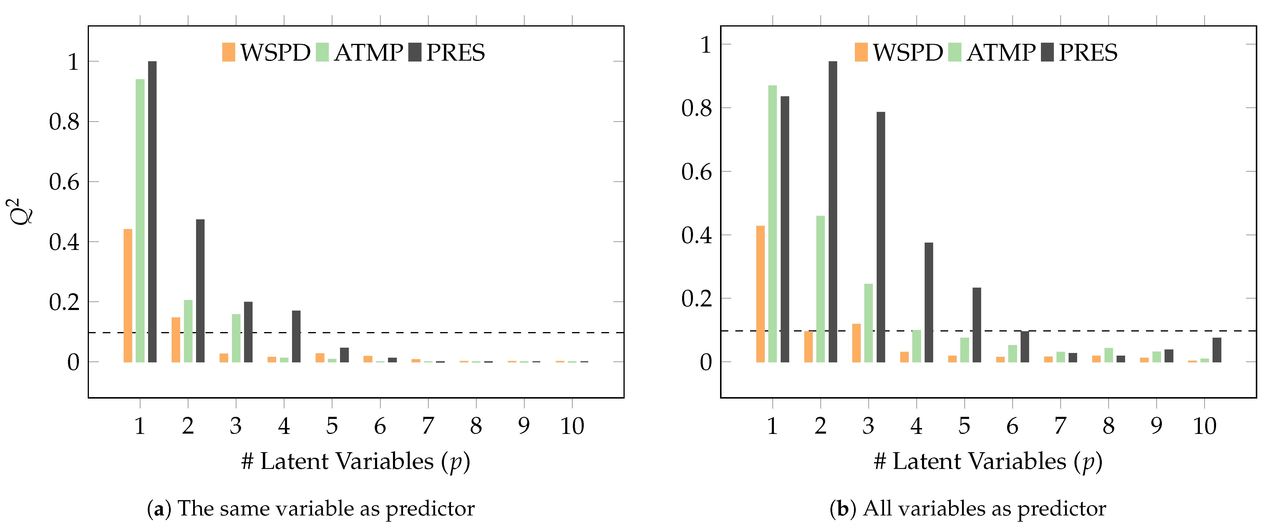
Figure 9a shows the values of
in function of the number of latent variables, in the case of predictions with the same meteorological variables. It can be observed that the number of latent variables that verify the criterion (
29) is two for the WSPD meteorological variable, three for the ATMP variable and four for the PRESS variable.
Similarly,
Figure 9b represents the values of
in function of the number of latent variables, in the case of predictions with all the meteorological variables. It can be observed that the number of latent variables that verify the criterion (
29) is now three for the variable WSPD, three or four for the ATMP variable and six for the PRESS variable.
Table 3 shows the errors obtained in the prediction of the variables WSPD, ATMP and PRES, of the PPX station, with the PLSAnEn, PLSClustAnEn and PLSR methods, for the cases where a different number of latent variables (LVs) are used as predictors, chosen according to the previously discussed criteria. As in
Section 4, the prediction/reconstruction period is the year of 2021 (restricted, everyday, to the same period—10 a.m. to 4 p.m.) and the remaining years, from 2016 to 2020, make up the training period. For each number (
p) of predictor LVs, and each method, the smallest errors are highlighted in bold.
In agreement with what was also observed in
Section 4, the use of all variables as predictors did not bring any advantages, and the errors obtained were smaller for predictor variables corresponding to the same meteorological variables being predicted. It may also be concluded that the increase in the number of LVs does not always translate into a smaller error in the reconstructed/predicted values; for instance, the errors obtained for ATMP were higher with four LVs, rather than with three. The PLSAnEn method exhibited the best results in the reconstruction/prediction of WSPD. The PLSR method exhibited the smallest errors in the reconstruction/prediction of PRES and ATMP, with results not far from those produced by the PLSAnEn method (for WSPD and ATMP).
6. Results
In this section, we examine the errors resulting from the data reconstruction using data from neighboring stations. The results are divided into two subsections:
Section 6.1, featuring the prediction of the station PPX, and
Section 6.2, which focuses on the reconstruction of each station contained in the dataset. As in previous sections, the reconstruction period is the year of 2021 (only the daily period from 10 a.m. to 4 p.m.) and the remaining years, from the beginning of 2016 to the end of 2020, constitute the training period. For each meteorological variable, all reconstruction/prediction methods were applied with the optimal number of PCs or LVs determined in the two previous sections.
Table 4 contains the number of PCs or LVs used by each method. As shown in
Table 2, ATMP reconstruction using the PCR method obtains better results when all meteorological variables are used as predictors. For this reason, this is the only case where the PCs (
) are obtained from all
original predictor variables. In the remaining cases, both PCs and LVs are obtained from predictor variables corresponding to the same meteorological variable that is predicted, i.e., PRES is predicted from PRES and WSPD is predicted from WSPD and GST, as shown in
Table 4.
6.1. Reconstruction of Meteorological Variable in One Station
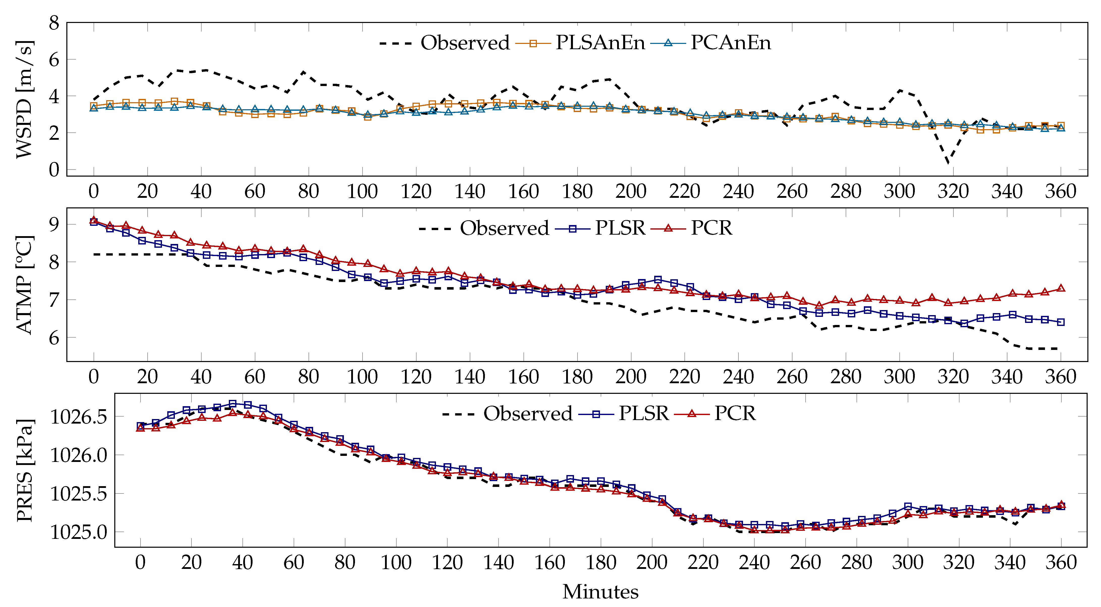
Figure 10 makes it possible to compare the real/observed values with the reconstructed/predicted ones, for the three meteorological variables, at the PPX station, in 9 January 2021, from 10 a.m. to 4 p.m. Only the values obtained by the methods with the smallest errors in
Table 2 and
Table 3 are presented. It can be seen that the WSPD variable varies much more in time than ATMP, and especially in comparison to the PRES variable. Visually, WSPD exhibits more variance at higher frequencies, i.e., more fluctuations between consecutive records.
For the WSPD variable, the reconstructed values are not able to reproduce specific variations. However, they reproduce the general trend of variation of the variable. It should be stressed that this meteorological variable undergoes permanent changes over time. These changes are greatly influenced by factors inherent to the location, such as the orientation and topography of the site. It can also be seen that there are no major differences between the values reconstructed by the PCAnEn and PLSAnEn methods.
For the ATMP variable, the values obtained by the PLSR method are closer to the observed values than those produced by the PCR method. Both sets of values exhibit some distance in relation to the observed values. In this geographic region (San Francisco bay area), there are persistent meteorological effects, namely the northern Oregon–California coastal jet [
37], coupled with the summer sea breeze [
38]. The spatial distribution of temperature is dependent on how inland the meteorological stations are located. Despite the spatial correlation shown in
Figure 5, the PCR method is worse than PLSR in reproducing the tendencies in temperature evolution.
The values reconstructed by the PLSR and PCR methods for PRES are very close to the observed values. Firstly, this meteorological variable is highly correlated over the spatial region of interest (c.f.
Figure 6); hence, the tendencies of the signals are similar. This is both a consequence of the stations being located at similar altitudes (near sea-level) and as pressure spatial variations are smooth. Secondly, its signal exhibits lower high-frequency fluctuations when compared to the wind speed signals. Both of these characteristics contribute to the performance of the reconstruction methods.
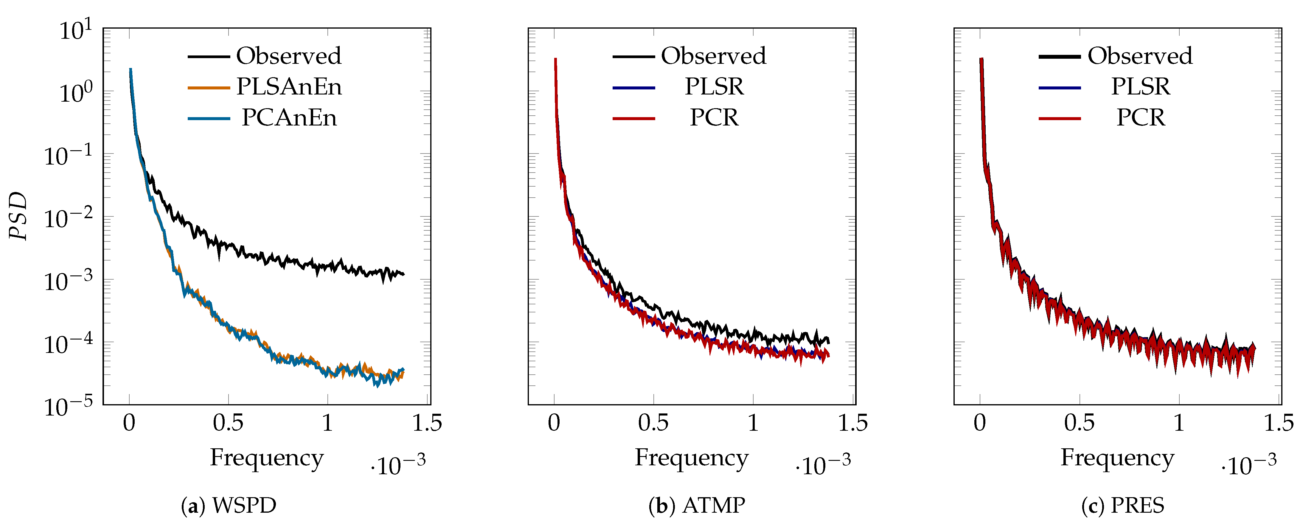
Although
Figure 10 presents a one-day comparison of predicted and observed values, it is insufficient to conclude that these patterns remain constant throughout the entire time series (1 year). Thus, an analysis is necessary to verify the consistency of these patterns in the complete dataset. To evaluate the prediction methods’ ability to capture high-frequency patterns, the normalized power spectrum densities (PSDs) [
39] of both reconstructed and observed series are compared in
Figure 11. Upon initial observation, the WSPD data display greater high-frequency density than that of ATMP and PRES. Generally, at low frequencies, the methods’ densities align with the observed data across all variables. However, for WSPD, the predictions fail to accurately capture the observed high-frequency variance. In contrast, for ATMP and PRES, the reconstructions exhibit similar high-frequency variance to the observed data. These results corroborate the previous one-day analysis.
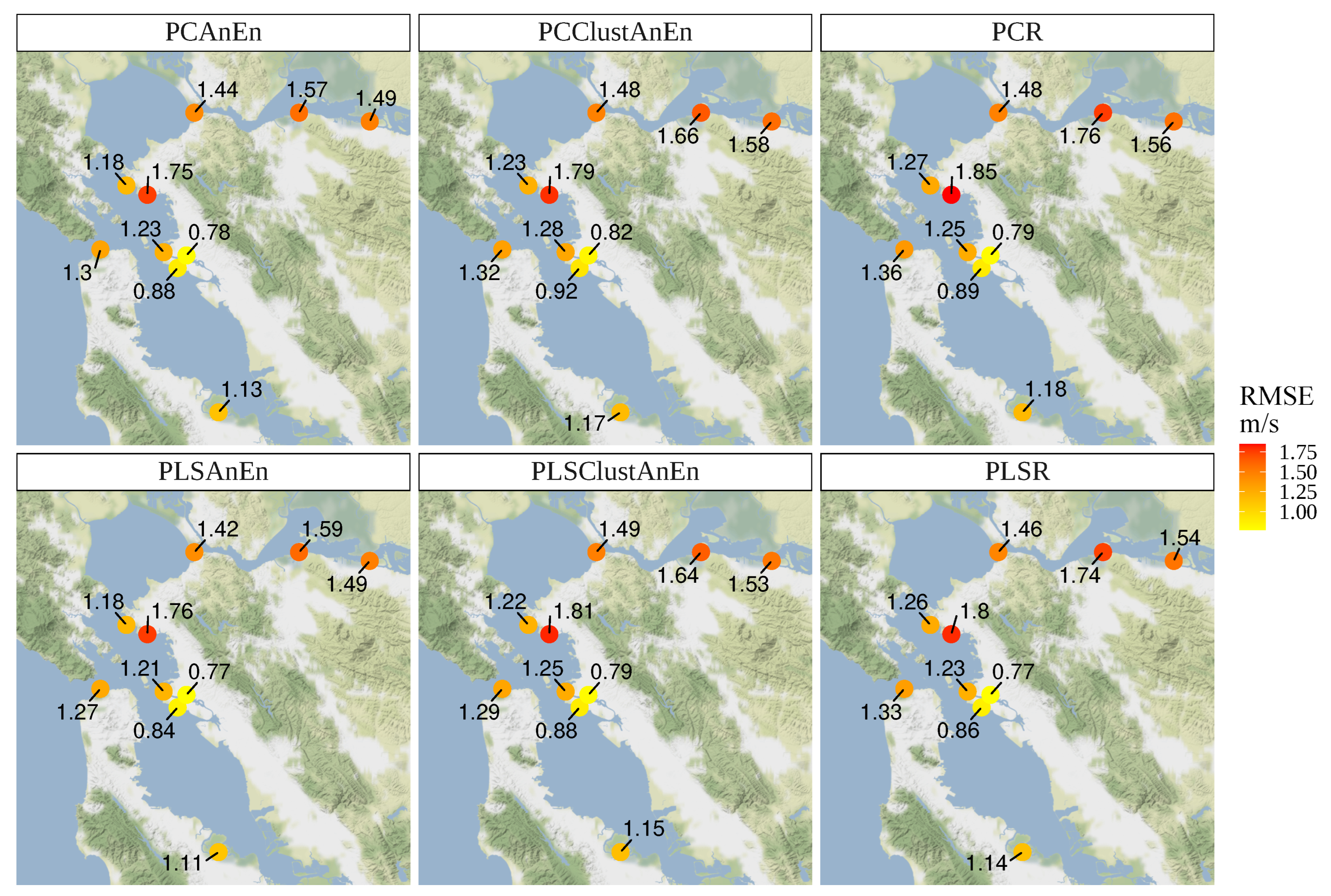
6.2. Reconstruction of Meteorological Variable in All Stations
Figure 12 shows the values of the RMSE errors per station, resulting from the reconstruction of the WSPD meteorological variable by the different methods. For all methods, it is observed, in general, that the lowest errors are obtained for the stations that occupy central positions in relation to the others. In general, it is also observed that PLS-based methods obtain lower errors than PC-based methods, although the differences are small (on the order of a tenth or a hundredth of a unit). The PLSAnEn method presents the best results in the reconstruction of the WSPD in all meteorological stations.
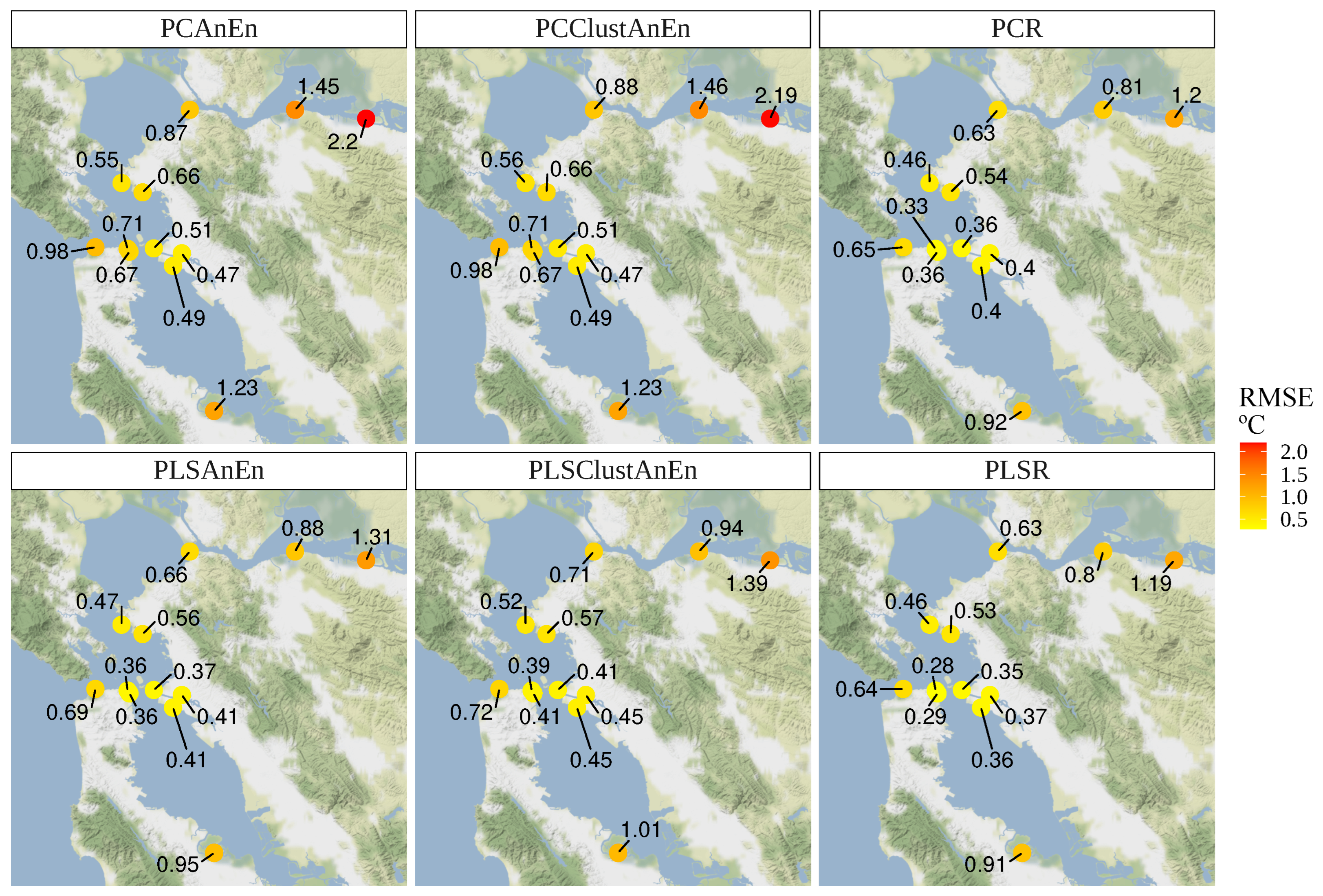
In
Figure 13, it is possible to observe the values of the same error for the reconstruction of the ATMP variable. In general, the errors obtained are smaller than in the case of WSPD. Here, also, the highest errors are obtained in the most peripheral stations, which have less correlation with the remaining. For this meteorological variable, the supremacy of methods based on the PLS method is also verified. The best results at all stations are obtained by the PLSR method, followed closely by the results obtained by the PLSAnEn method.
Finally,
Figure 14 also shows the RMSE errors, this time during the reconstruction of the meteorological variable PRES. The low error values show that PRES is clearly the easiest variable to reconstruct. In this case, PLS-based methods do not always obtain the best score, which is achieved by the PLSR method. Following PLSR, the method that obtains the best results is PCR, especially in the most central stations. The PLSAnEn and PLSClustAnEn methods obtain the same results at all stations.
7. Computational Performance
This section analyzes the computational performance of the reconstruction methods considered in this study. The computational system used for the evaluation was a virtual machine hosted in a KVM-based virtualization cluster, with the following characteristics: 16 cores of an Intel Xeon W-2195 CPU, 64 GB of RAM, SSD-based local storage, Ubuntu 20.04 operating system, R version 4.2.2 (all tests were implemented in the R language [
40]).
Table 5 presents the mean execution times, in seconds, needed by each method in the reconstruction of the meteorological variables for all the different stations analyzed in the previous section (each execution time presented in the table corresponds to the average of the times of all stations). These execution times concern the execution in a parallel regime (by instructing the R platform to exploit, whenever possible, all the available CPU-cores).
The execution times are broken down into three consecutive stages: loading, decomposition (PCA or PLS) and prediction/reconstruction. The loading stage corresponds to the reading of the data set from CSV files and interpolation of missing values (when they are not more than four consecutive values). In the case of the reconstruction of WSPD, the loading step involves the reading of both the WSPD and GST dataset files, which takes ≈37.2 s; even longer, the loading of the ATMP dataset, when using the PCR method, takes ≈61.2 s because this method uses all 37 predictor variables (recall
Table 2).
The PCA or PLS decomposition step corresponds to the calculation of PCs or LVs, respectively. This step is conducted by internal R functions that are already highly optimized from a computational point of view. As such, the execution time of this step is very fast (however, this step can include also the choice of the number of components through the LOOCV method, which may have some computational costs).
The final step consists of the reconstruction/prediction of the missing values. In the PCR and PLSR methods, this stages executes very fast, through linear regression with previously determined PCs or LVs. However, for PCAnEn and PLSAnEn, this stage is very demanding because, for each value to be reconstructed/predicted, the training period is swept in search for analogs. In turn, for the PCClustAnEn and PLSClustAnEn methods, this step is not as demanding, once all possible analogs are previously clustered, and the sweeps are reduced to a single operation in which the predictor value is compared with the cluster centroid. Overall, the slowest methods are thus the PCAnEn method (WSPD) or the PLSAnEn method (ATMP and PRES) and the faster (for all variables) is the PLSR method.
The execution times presented in
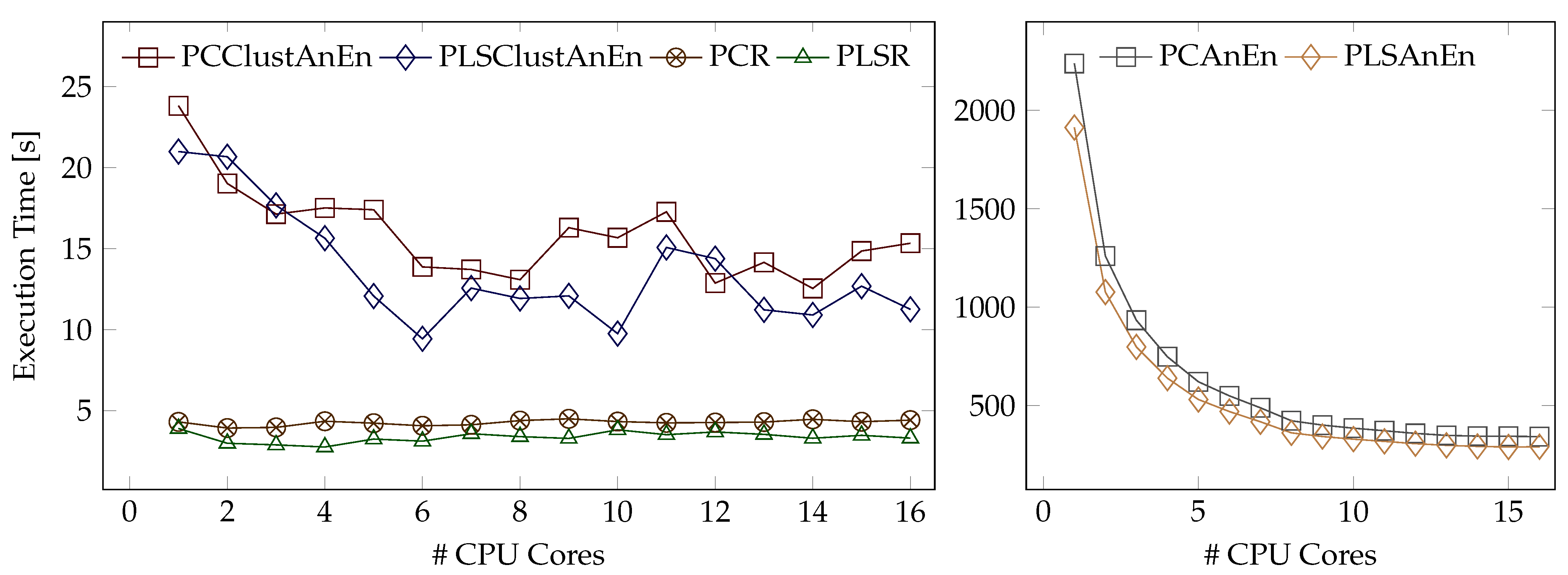
Table 5 were obtained using all CPU-cores available. The impact of using a varying number of CPU-cores may be apprehended by inspecting
Figure 15. This figure represents the execution time for the reconstruction of WSPD in station PPX in function of the number of CPU-cores, without including the loading time (more IO-sensitive). In these experiments, PLSR and PCR cross-validations were parallelized to accelerate the 10-fold LOOCV process. It can be seen that the PCR and PLSR methods perform similarly for any number of CPUs. In turn, the PLSClustAnEn and PCClustAnEn methods benefit from increasing the number of CPU-cores, especially up to 6/8; however, as these methods depend heavily on the clustering phase of possible analogs, which is not always performed in the same number of iterations, their performance does not always improve with the increased calculation capacity.
Regarding the PCAnEn and PLSAnEn methods (right sub-figure), it may be observed that they are more sensitive to the increase in the CPU-cores employed, with their computational efficiency improving when using up to about ≈10 cores. It turns out that these methods are highly parallelizable: many searches for analogs may be carried out simultaneously once they are inherently independent from each other. However, despite the performance gains brought by the parallel execution, the PCAnEn and PLSAnEn methods are still considerably slower than the others.
8. Conclusions
This study presents methods that allow for solving hindcasting and forecasting problems with a high number of predictors. Solving these problems with a large number of predictors using the classical analog ensemble methodology, though feasible, is very inefficient, due to the magnitude of the computational load involved.
The methods presented here combine the robustness of the AnEn method (with or without clustering) and the PCA and PLS techniques for dimension reduction of the predictor dataset. Using these techniques, the predictor variables are reduced to a small number of new variables that mostly retain (PCA) and may even enhance (PLS) the meteorological information used by the AnEn method to reconstruct or forecast the records sought.
The results produced by the PLS-based techniques were found to be slightly more accurate than those obtained with the PCA-based ones, especially in the reconstruction or forecast of meteorological variables with a significant amount of oscillation, such as wind speed (WSPD). This happens because PLS builds the latent variables in such a way that they simultaneously explain the variation of the predictor variables and the predicted variable, while the main components, obtained by PCA, only explain the variation of the predictor variables.
The combination of the AnEn method with PLS results in a hybrid method, PLSAnEn, which makes it possible to accurately reconstruct or predict the wind speed. It is therefore a highly suitable forecasting method for meteorological time-series with potential applications in wind-resource assessment and wind energy. At the same time, PLSAnEn is very demanding from a computational point of view, which benefits from a parallel implementation.
PLSClustAnEn, which combines the AnEn methods with the prior clustering of analogs, could be an alternative to the PLSAnEn method, as it is much more computationally efficient. It is, however, a method that depends on many parameters that have to be properly chosen in order to improve the accuracy of the results.
Simultaneously with the AnEn-based methods, regression methods were also tested on the new variables determined by PCA or PLS. The resulting methods, PCR and PLSR, are very fast and allow for very accurate reconstructions. In particular, the PLSR method is the most suitable for reconstructing or forecasting highly correlated predictor variables.
In the sequence of this work, we intend to apply the proposed methods to industrial problems, related to renewable energies, such as forecasting, downscaling or reanalyzing, where there is a need to address a large number of predictor datasets.


