1. Introduction
The primary factors that influence sovereign bond yields are typically domestic macroeconomic and financial fundamentals, as well as global factors such as international risk appetite and global liquidity [
1], as indicated by a substantial body of literature (see, among others, [
2,
3]). Credit ratings are widely regarded as a standard means of measuring a country’s financial risk and play a critical role in assessing its overall risk profile [
4]. Furthermore, international investors seeking to realize higher returns inevitably face higher risk and volatility and scarce relevant information when focusing on emerging markets [
5]. As a result, they turn to credit ratings as valuable indicators of a country’s capacity or willingness to meet its financial obligations. Hence, credit ratings can also be seen, as Cantor and Packer (1996) suggest, as a reflection or proxy of domestic macroeconomic and financial indicators. If a financial market is fully efficient (in the strong sense) and there are no delays in the dissemination of information, rational market participants (as suggested by [
1,
2]) would have already factored in any changes in a country’s fundamentals since the information is considered to be available to participants at the time of the credit issuance. Nevertheless, especially concerning emerging markets, information, in reality, is scarce, and as literature suggests [
6], credit ratings convey some kind of extra information to markets and do have an effect on spreads [
7]. Multiple studies [
1,
8] have yielded consistent results indicating that yield changes are more strongly impacted by negative rate changes, particularly shifts from investment grade to speculative grade, as opposed to upgrades. It should not be forgotten, though, that there is also a regulatory (Basel III Accord) reliance on credit ratings or sometimes an internal corporate policy that forces institutional investors, such as retirement and insurance funds [
1], to invest exclusively in securities that enjoy an investment grade.
The objective of this study is to evaluate two complex economic and social phenomena that have not been adequately explored in previous research as potential influencers of sovereign credit ratings and bond yields. The two phenomena under consideration are the prevalence of information and communication technologies and the market-driven economic changes arising from the existence of a shadow economy. The motivation for this study should be attributed to the work of Elgin and Uras [
9] concerning the shadow economy and Bissoondoyal-Bheenick et al. [
10] regarding ICT, which, to the best of our knowledge, first introduced the two phenomena in the relative literature.
Elgin and Uras [
9] (see also Markellos et al. [
11]) provided empirical evidence that economies with large informal sectors have a greater propensity to default. Inevitably, diminished public revenues lead to fiscal deficits that a government has three ways to finance: increase tax rates, posing the risk of prompting more businesses to shift to the shadow economy, resulting in reduced overall revenues; cutting down on public expenditures, running the risk of compromising the quality and range of public goods and services offered to citizens; and issue and sell more debt, risking an increase in its cost [
12].
The link between the transformation of economies to economies of knowledge through ICT was intuitively recognized by Bissoondoyal-Bheenick et al. [
10], who claimed that given that the diffusion of ICT (the informational technological capacity was proxied by the use of mobile phones) shapes the future, the assessment of future creditworthiness should be determined to a certain degree by the level of ICT use. In this line, although no direct effect was found, Kotzinos et al. [
13] proposed that ICT is an important indirect driver of sovereign ratings and interest rates by facilitating economic growth and improving labor productivity, while the indirect effect seems to be larger for the leapfrogging developing countries.
Interestingly, some researchers [
14,
15] have shown academic interest in the link between internet penetration (which forms a significant aspect of the ICT revolution) and the size of the shadow economy. Their research has revealed a negative correlation that is particularly pronounced in the developing stage (as indicated by GDP per capita). In this paper, we undertake a comprehensive examination, for the first time, of the relationship between ICT and the shadow economy with respect to both sovereign ratings and the cost of debt, both separately and in conjunction. We attempt to form an understanding of the aforementioned links through a series of non-parametric machine-learning approaches. Machine learning algorithms, while an established workhorse (along with logistic regression) method concerning financial institution decision processes have not seen a proportional spread in academic literature related to the sovereign cost of debt. This is mainly because the focus of this literature is on comprehending the underlying mechanism rather than solely on prediction. Most machine learning algorithms have long been considered “black boxes” [
16] and therefore unsuitable for providing information on the structure of the relationship between dependent and independent variables. The evolution of model intrinsic and model agnostic interpretability methods [
17] allows the shedding of light on the underlying mechanism of machine learning algorithmic predictions.
Our analysis offers a continuation of the current empirical literature by providing additional insights into the significance of ICT diffusion and the size of the informal economy as factors influencing ratings and rates. Furthermore, it is the first to explicitly examine the potential additional impacts of these two variables while considering their primary effects. Secondly, our study suggests the utilization of recurrent neural networks, which are highly flexible, able to approximate non-linear relationships and deliver very promising results. Thirdly, we utilize state-of-the-art methods that make the behavior of the machine learning models somewhat explainable, enabling us to describe and quantify the effects being studied. Fourthly, this research adds to the crucial discussion regarding the significant role that ICT and the informal economy play in contemporary societies.
The rest of the paper is organized as follows:
Section 2 reviews the literature, focusing especially on the economic repercussions of the two phenomena that rating agencies and markets might take into consideration.
Section 3 presents the empirical analysis.
Section 6 provides some discussion on findings and policy implications, and finally,
Section 7 concludes.
3. Empirical Application-Data and Sources
Our credit risk sample consists of 1029 (there are 11 country-year credit ratings missing, more specifically ratings concerning Moldova and Nicaragua and years 2011–2016). If no missing ratings existed in the sample, observations would amount to 1040 annual (end of the calendar year) observations of long-term foreign currency credit ratings of sovereign bonds assigned by Standards and Poor’s rating of sixty-five countries (countries comprising our sample classified by region and development stage can be found in
Table A5 of
Appendix A.) for a time period of 16 years (2001–2016). Qualitative letter ratings are linearly transformed to numerical equivalents, with 1 representing the highest score (triple A) and 21 the lowest (default). As a result, a rise in the rating indicates a country’s downgrading. We opt for Standard and Poor’s rating among the major three rating agencies that dominate the market (the others are Fitch and Moody’s) since there is some evidence in the literature [
40] that S&P acted as a rating setter during the recent crisis and that downgrade announcements of the specific agency carry increased importance for markets. In any case, we do not expect our findings to be driven by the agency choice due to the close correspondence of the three agencies [
41] and the extremely high pairwise correlation coefficients found in our sample concerning them (over 0.970 in all cases).
The sovereign cost of debt is proxied by the yield to maturity of the ten-year zero-coupon sovereign benchmark bonds; if this is not available, the closest maturity is chosen. If such data were completely unavailable, we filled, wherever possible, the dataset using the JP Morgan Chase Emerging Markets Bond Index Global (EMBI Global), which tracks total returns for traded external debt instruments in emerging markets (definition from
https://cbonds.com/glossary/emerging-markets-bond-index/, accessed on 25 December 2022). The cost of debt sample comprises 862 observations of sixty-one countries for a time span of 2001–2016 (on this occasion, there are 114 missing county-year observations).
The independent variables, and the focus of interest in this study, are ICT penetration and the extent of the shadow economy across countries. ICT penetration and usage among countries are measured by the NRI composite index (network readiness index). The index was not published for years 2017 and 2018 and was redesigned in 2019 by the Portulans Institute, losing its consistency. It was first published in 2002 (involving the year 2001) and aims to measure the multitude of ICT aspects that have an impact on economic development and society by assigning a score on a scale from 1 to 10, with the latter being the best possible grade. The index was, until 2016, published by the World Economic Forum, Cornell University, and INSEAD (The NRI, 2022), and therefore, despite some minor reviews, retained its consistency and suitability for use in a time-series framework. It should be noted, though, that concerning the year 2015, no assigned scores were published, and therefore we interpolated the missing values by using the inverse distance weighted method of non-missing values, with weights being reciprocals of the squared distance between values (since NRI scores do not change dramatically from year to year, this method allows for assigning more weight to the closest non-missing values). We expect higher values of the index to be associated with lower yields and better (lower) ratings.
The shadow economy estimates (% GDP) are those [
25]. (To the best of our knowledge, these are the latest and most updated estimates for 2017). In conjunction with the last consistent, in a time-series framework, publication of the NRI index (2016), the years under study cannot be significantly expanded. We expect higher values to be associated with increased yields and higher (or worse) credit ratings. Moreover, considering, on the one hand, the plethora of means that ICT delivers to the governments of developing countries to provide basic services and digitize parts of a fragile and vulnerable to corruption public sector and, on the other hand, the inverse relationship between ICT and shadow economies that is found in the literature [
14], we expect that improvements on ICT diffusion will alleviate the positive (increasing) effects of large shadow economies on sovereign ratings and debt rates.
Furthermore, we employ a set of key economic variables that have been spotted in relative literature [
8,
42,
43] as determining the capacity and willingness of borrowers to service their debt [
44] along with factors capturing global conditions such as risk sentiment (VIX) and liquidity (risk-free U.S. rate). We include the specific variable only in bond yield models because it is not commonly included in modeling sovereign ratings in the relative literature.
Moreover, we use a set of dummy variables (mostly time-invariant) in order to capture a country’s classification as an advanced or developing economy (
advanced) (a definition taken by the Country Composition of World Economic Outlook Groups in 2012), eurozone membership (
eurozone), a default after 1995 (
dflt95), or common or civil origin of law (
lgluk) (an abbreviation of the corresponding proxy binary variable). Countries with common law origin take the value of 1, zero otherwise, and regional effects (
West/Latin-Carribean/East Europe/Asia-Pacific/Africa/Middle-East) (binary indicators for region indicator). See
Table A5 of
Appendix A for a complete presentation of sampled countries by stage of development and region. Additionally, a dummy variable proxies the period of extreme stress in global financial markets between 2007–2010. Definitions of numeric explanatory variables, sources, and expected impact signs are shown in
Table A3 of
Appendix A, and overall descriptive statistics are shown in
Table A2 of
Appendix A.
When assessing the determinants of the cost of debt, we employ ratings as an independent (when employing credit ratings as an independent variable, we prefer a synthetic proxy constructed as the simple average of the assigned ratings of S&P, Moody’s, and Fitch because there is no reason to believe that investors will not take under consideration, in a distinct but unknown to us ratio, all available information and therefore all assigned sovereign credit ratings by the three agencies, if of course available.) variable is driven by the “extra” information they might convey beyond economic fundamentals.
Table A4 of
Appendix A gives the Pearson correlation coefficients of dependent and explanatory variables. Notably, yields are mainly correlated (negatively) to ICT penetration and labor productivity and positively to assigned ratings, inflation, the shadow economy, and corruption. On the other hand, S&P ratings (and also a synthetic metric based on the average ratings of S&P, Moody’s, and Fitch) are strongly (negatively) correlated to ICT penetration, labor productivity, and credit to the private sector, while positively correlated to corruption, the informal economy, and inflation. ICT penetration is strongly (positively) correlated to credit to the private sector and labor productivity and negatively to corruption and informality, which are also strongly and positively correlated between them.
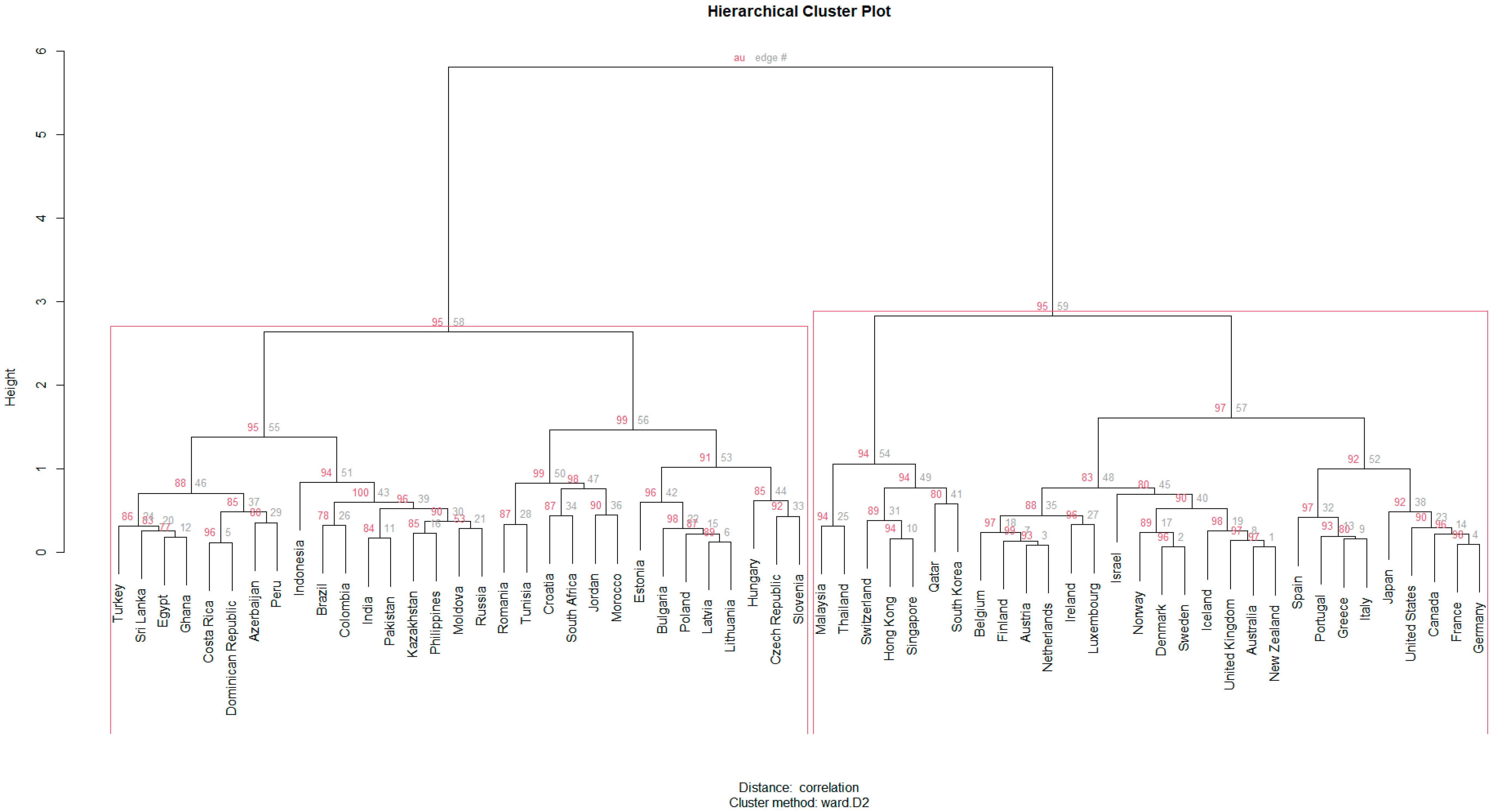
Before proceeding with the main analysis and in order to secure the robustness of our models, we test to find out whether the set of employed independent variables (including ratings; here we employ the average of the assigned ratings by the three agencies since it constitutes public information, since this piece of information is also available to market participants) is able to discern between groups of countries of different creditworthiness or if we encounter an omitted-variable bias. For that purpose, we employ hierarchical clustering, an alternative to the k-means clustering approach that has the advantage of not needing a pre-specification of the number of clusters. Before applying the approach, all numeric variables are collapsed to their country means and scaled. Binary factor variables are set to their modes. The algorithm works in a bottom-up manner (agglomerative clustering), meaning that each country is considered a leaf (a distinct cluster), and at every next step, the pair of clusters with the minimum between-cluster distance are merged (Ward’s method) until we end up with only one cluster (the root).
The dissimilarity between any two observations is measured by the parametric correlation distance, which is defined by subtracting the correlation coefficient from 1 and takes the following form:
The distances are squared before cluster updating [
45]. The cluster dendrogram generated along with approximately unbiased “
p-values” of clusters’ support, calculated by multiscale bootstrap resampling, can be seen in
Figure 1.
The two large groups (no. 56 and 57), generally corresponding to developing and developed countries, can be easily discerned and are strongly supported by the data (au >95%). However, this clustering is not very helpful in order to correctly identify the average expected cost of debt that a country will cope with, depending on its specific characteristics. Nevertheless, it can also be observed that with adequate confidence (au >= 94%), four distinct groups (no. 54, 55, 56, and 57) may be formed to provide us with quite a satisfactory clustering:
- ○
Cluster 57: Australia, Austria, Belgium, Canada, Denmark, Finland, France, Germany, Greece, Iceland, Ireland, Israel, Italy, Japan, Luxembourg, Netherlands, New Zealand, Norway, Portugal, Spain, Sweden, United Kingdom, United States.
- ○
Cluster 54: Hong-Kong, Malaysia, Qatar, Singapore, South Korea, Switzerland, and Thailand.
- ○
Cluster 56: Slovenia, Czech Republic, Estonia, South Africa, Croatia, Poland, Latvia, Hungary, Lithuania, Romania, Bulgaria, Tunisia, Jordan, and Morocco.
- ○
Cluster 55: Azerbaijan, Brazil, Colombia, Costa Rica, Dominican Republic, Egypt, Ghana, India, Indonesia, Kazakhstan, Moldova, Pakistan, Peru, the Philippines, Russia, Sri Lanka, and Turkey.
As we can see, the first group refers to countries that are considered to belong to the “West” or have successfully adopted Western-type institutions (e.g., Japan, and Israel). The second cluster comprises highly dynamic Asian economies with skilled labor and semi-democratic institutions, along with Switzerland and Qatar. These two clusters are expected to be able to borrow with ease when needed. The third cluster consists mainly of ex-communist European countries rising rapidly along with African or Middle Eastern countries (South Africa, Tunisia, Jordan, and Morocco) that are more developed relative to their neighbors. This group is expected to attract investors through increased yields since it carries a higher risk than previous clusters. The last group is a mixture of South American, Eastern European, African, Asian, and Middle Eastern sovereigns that have a history of severe economic turbulence or defaults, and an unstable political environment and are obliged to cope with increased borrowing costs. Overall, the determinants seem to be able to distinguish, at least in broad terms, the different levels of credit risk depending on countries’ specific traits and permit us to consider the choice of independent variables as adequate.
4. Non-Parametric Analysis of Sovereign Credit Risk
When we have a dataset and need to answer questions using machine learning techniques, it is typical to use multiple approaches and evaluate their effectiveness, according to Boehmke and Greenwell [
45]. A possible convergence of findings among different algorithms could lend us some confidence in our outcomes. Machine learning approaches are especially appropriate when dealing with complex situations [
11] that lack a sound economic theory. The study (concerning empirical methods applied) that is closer to ours is that of Bennel et al. [
44] (see also [
46]) that applies several artificial neural networks on a 16-point (classes) scale of 1383 annual observations assigned by eleven rating agencies; they manage to achieve a correct classification rate of 42.4% or 67.3% if predictions within one notch of the true rating are taken as correct. We employ these rates as the benchmark for our models since other similar studies have artificially limited the number of classes and therefore are not comparable to the present study.
4.1. Classification Trees and Bagging on Credit Ratings
Classification trees partition a dataset through an iterative process that splits the data into homogeneous subgroups and then splits those subgroups (or branches) further until a certain criterion is met, a procedure known as binary recursive partitioning. Splitting the data randomly when constructing the train and the test set may cause data leakage since the time dimension would be ignored and we would try to forecast the past while we stand in the future, achieving an inflated rate of correct/near correct predictions. Therefore, we split our sample into two sequential periods: the first consists of years 2001–2013 (81.5% of total observations) and forms the training and validation set, and the second of years 2014–2016 (19.4% of total observations) and forms the testing set. Following a CART approach (classification and regression tree, developed by Breiman [
47]), and after conducting a grid search in order to optimize the model’s parameters, we set the minimum number of observations that must exist in a node in order for a split to be attempted to 25, the maximum depth of any node to 9 (the root node counted as 0), and define that any split that does not improve fit by 0.01 will be pruned.
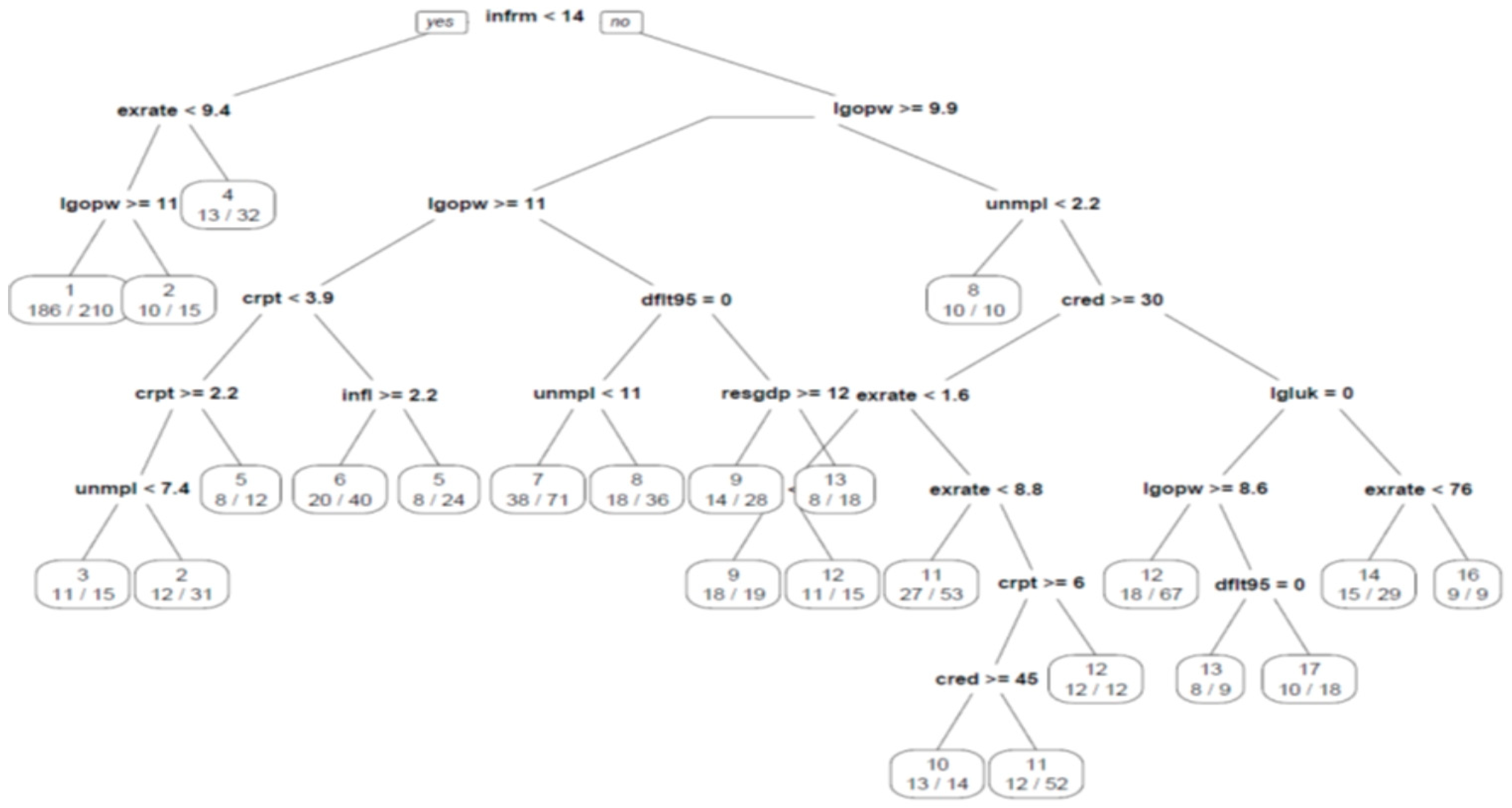
Figure 2 visualizes the generated classification tree that uses 24 final nodes and a depth of eight levels to achieve a 55.54% (computed as relative error*Root node error) correct classification rate concerning the training set and a rate of 48.2% on the testing set, which is quite satisfactory.
The default splitting criterion is the Gini index. (Alternatively, information gain can be used as the splitting criterion, but the classification rate does not improve substantially.) This is calculated by subtracting the sum of the squared probabilities of each class from one; therefore, it is defined as
and equals zero in the case of perfect classification. As we can see in
Figure 2, the size of the shadow economy (<14% of GDP) is the chosen feature basis of the root node. Given that a country confines the informal sector below 14% of GDP, if the local currency exchange rate to one US dollar is above 9.4 local units, the most probable anticipated assigned rate would be (AA-).
If, on the other hand, the local currency is stronger and, concurrently, output per worker equals or surpasses 59,784.14 constant 2010 USD per annum, the model predicts an AAA rating, otherwise an AA+. All branches of the presented tree can be read in the same way.
Additionally, to gain a deeper understanding of the factors influencing a model’s prediction (we note that a variable may score high without necessarily appearing in the tree [
48]), we can measure the importance of the explanatory variables by summing the squared improvements across all internal nodes of the tree where each feature was selected as the partitioning variable, according to Boehmke and Greenwell [
45]. To gain a deeper understanding of the factors influencing a model’s prediction, we can measure the importance of the explanatory variables by summing the squared improvements across all internal nodes of the tree where each feature was selected as the partitioning variable, according to Boehmke and Greenwell [
45]. The relative importance of the explanatory variables of our tree classification model is shown in
Figure 3. While the classification rate of our optimal classification tree is quite satisfactory for a classification problem concerning 20 classes, single-tree models are notorious for suffering from high variance, i.e., small changes in the training set might cause great alterations to the model.
It has been proposed in the literature [
49] that one way to overcome this deficiency is to average the outcomes of multiple models. Therefore, we use the proposed by Breimann [
49] bagging (bagging stands for bootstrap aggregating) approach, which ultimately creates m bootstrap samples from the training set, and for each sample, a single, unpruned tree is trained while separate predictions from each tree are averaged in order to provide the finite predicted value.
This time, we repeat 10-fold cross-validation ten times in order to improve the estimation of the performance of our model. Following relative literature, the model’s performance improves significantly, not only concerning the cross-validation set, reaching a 70% correct classification rate, but more importantly, on the test set, achieving a rate of accuracy equal to 53.16%.
Relatively, the most important factors do not change dramatically, but we can discern that the CART method puts more emphasis on whether a country is considered advanced and whether it is a member of the “West”, while bagging relies more upon economic fundamentals.
Interestingly, ICT penetration and the size of the shadow economy are among the first four more important factors, with the most important being the workers’ productivity.
4.2. Classification Trees and Bagging on Bond Yields
Following the aforementioned methods, we split our sample into two sequential periods: the first consists of years 2001–2013 (78.8% of total observations) and forms the training and validating set, and the second of years 2014–2016 (21.2% of total observations) and forms the testing set. A ten-fold validation strategy is also implemented. A CART regression approach is similarly followed. After conducting a grid search in order to optimize the model’s parameters, we set the minimum number of observations that must exist in a node in order for a split to be attempted to 16, the maximum depth of any node to 12 (the root node counted as 0), and defined that any split that does not improve fit (overall R
2) by 0.01 should be pruned.
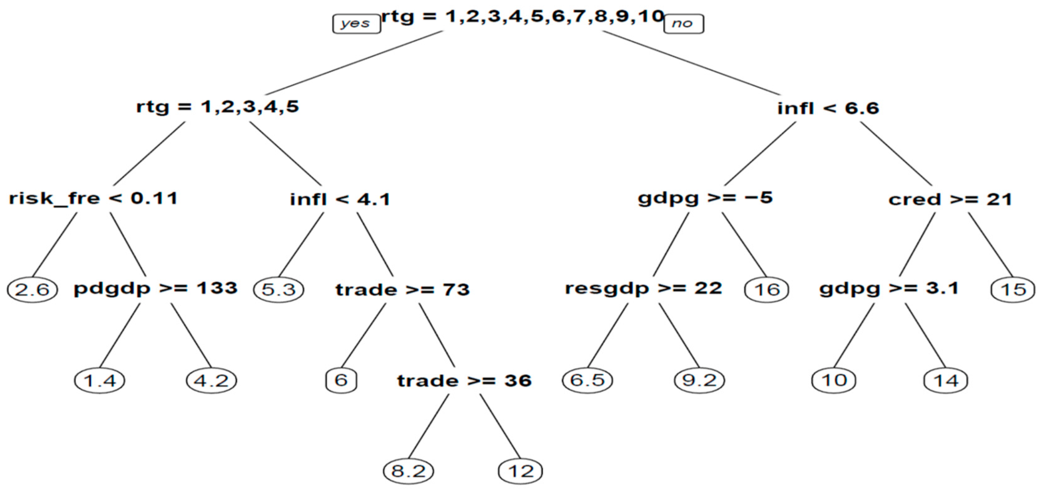
Figure 4 visualizes the classification tree that uses 12 nodes and a depth of three levels to achieve a training error of 2.44 (computed as relative error*Root node error) and a testing error of 2.824. The optimizing criterion is a reduction in the sum of the squares of the residuals (SSE).
As we can see in the graph, the credit rating is the chosen feature basis of the root node, and countries that are assigned a rating between AAA and A+ while at the same time, the global risk-free rate is lower than 0.11% should expect, on average, a yield of 2.6%. If the risk-free rate is equal to or exceeds 0.11%, then the yield also depends on the public debt-to-GDP ratio.
If the assigned credit rating is between A and BBB-, i.e., still in investment grade with strong or adequate payment capacity, the predictions are further split based on inflation and the country’s openness to trade. On the other hand, if a country is assigned a non-investment grade, the predictions are split based on GDP growth and reserves to GDP or credit to the private sector and GDP growth.
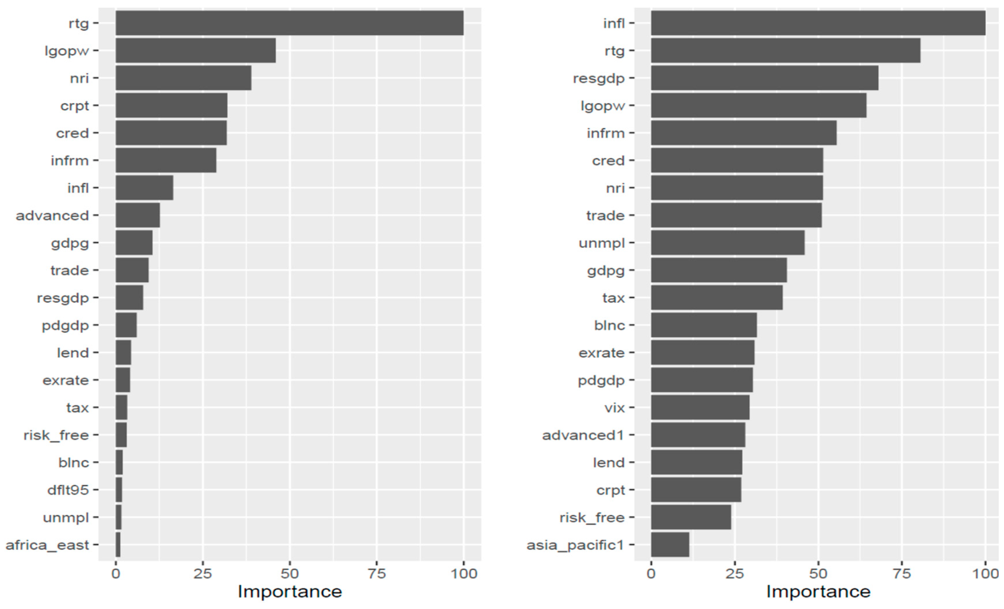
The relative importance of the explanatory variables of our tree regression model is shown in
Figure 5, along with a similar bagging model. As it is shown, the obvious most important feature (as expected) concerning the cart method is the assigned credit rating, followed by productivity per worker, ICT penetration, corruption, credit to the private sector, the magnitude of the informal economy, and inflation. The most noticeable difference between the two methods is that inflation and reserves relative to GDP are gaining importance with the bagging method.
ICT diffusion and the informal sector are still important drivers of sovereign yields in the bagging model. It can also be seen that the stage of development and the period of crisis (2007–2010) are not playing an important role in determining yields. We should note here that our bagging model fails to improve the test data error rate, which remains unchanged at 2.85.
4.3. Random Forests on Credit Ratings
According to Boehmke and Greenwell [
45], although bagging regression trees can be seen as an improvement over a single tree model, which tends to have high variance, they still have the issue of tree correlation. A modification and remedy to this problem is the random forest method, which seeks to de-correlate the m-bootstrap sample trees by injecting randomness into the tree-growing process by limiting the candidate for split variables to a random subset. Furthermore, random forest models provide a method to approximate the test error without the need to withhold training data for validation purposes by utilizing the left-out data from the m-bootstrap samples, which are known as out of the bag (OOB) samples. Before actually running the model, a handful of tuning parameters was set through an extensive grid search. Concerning the number of variables randomly sampled as candidates at each split, the optimal number was set to 4, the number of trees to grow to 500, and the complexity of the trees, which is adjusted through the size of the nodes, to 1 (the smaller, the deeper); the OOB error rate for these parameters amounted to 27.29%. The accuracy rate of our model on the unseen (test) data increased slightly relative to the bagging model and reached a more than satisfactory 57.89% with a rather remarkable accuracy within one notch of 84.21%.
Clearly, the model finds difficulties in the area around the boundary of investing-non-investing grade predicting investing grade rating (BBB/9) for eight non-investing grade observations (see
Table 1). An explanation could be that on this boundary, the assignment decision becomes even more subjective due to the profound implications.
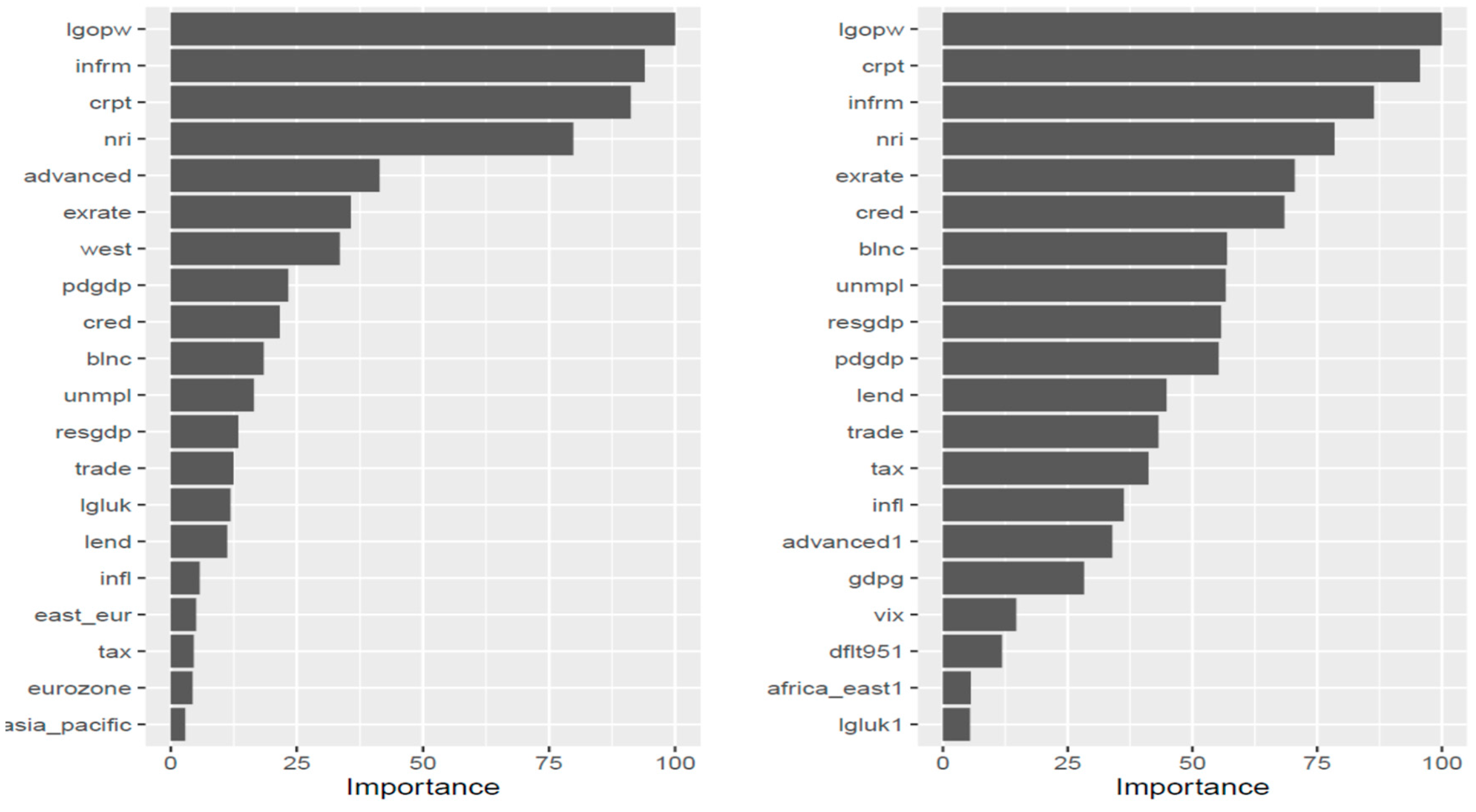
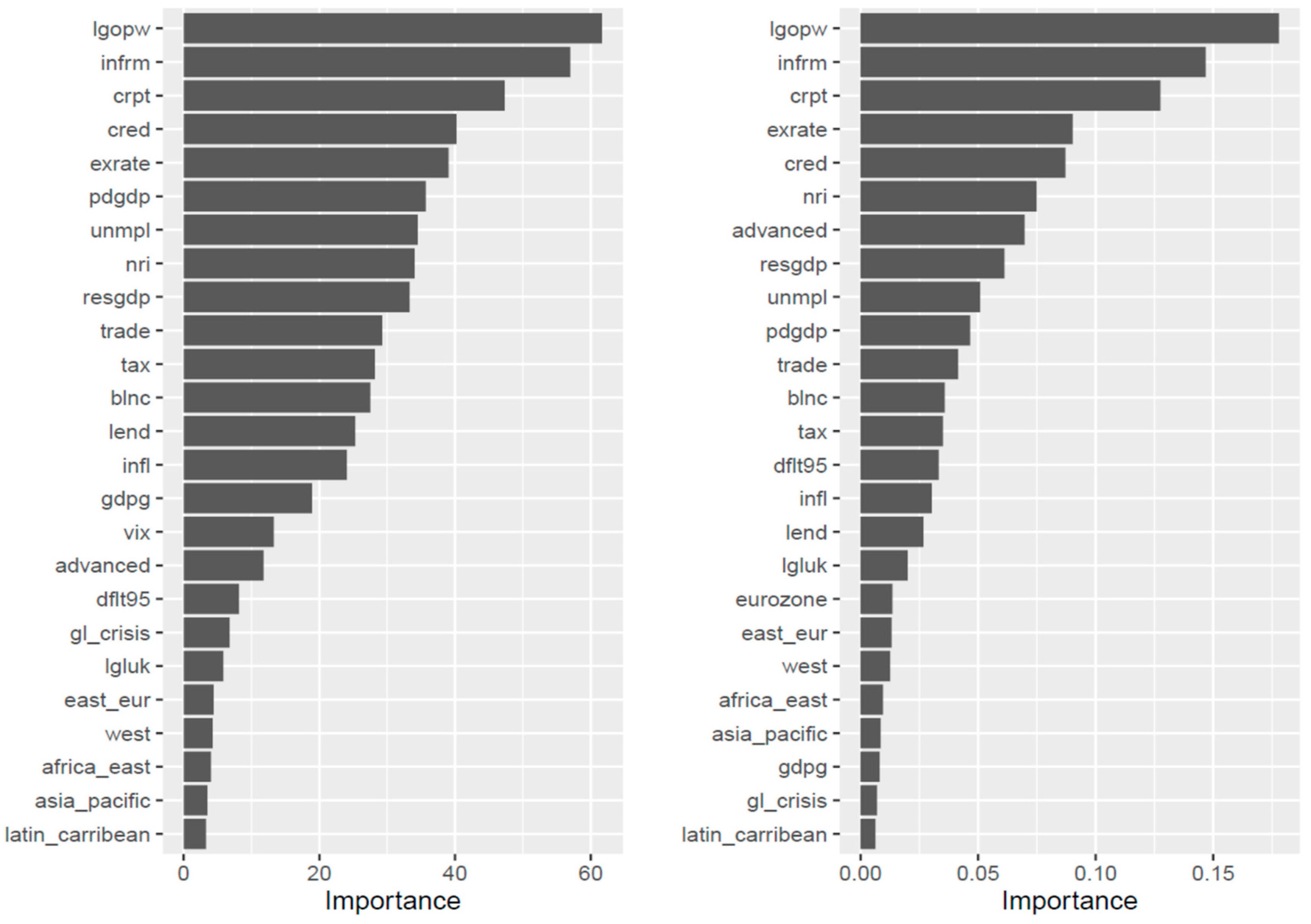
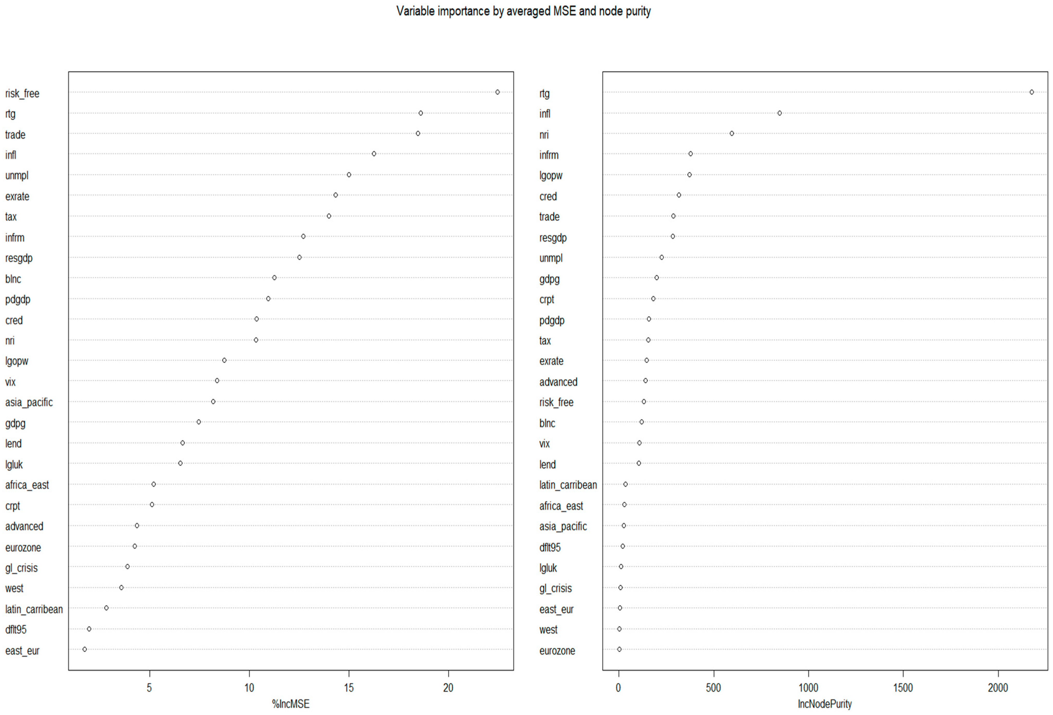
For verification reasons, we present two plots of the variables’ importance (
Figure 6): the one (left) based on the impurity measure, which is actually the Gini index for classification, and the permutation, which breaks any association between the variable of interest and the outcome by permuting the values of all observations concerning the specific variable, computes again the accuracy and then calculates the difference. The calculation is repeated for all the random forest model trees and averaged. It seems that the importance of the workers’ productivity is confirmed by the random forest model as well as by the size of the informal sector and corruption. ICT penetration appears to hold a moderate but still important place as a potential driver of credit ratings.
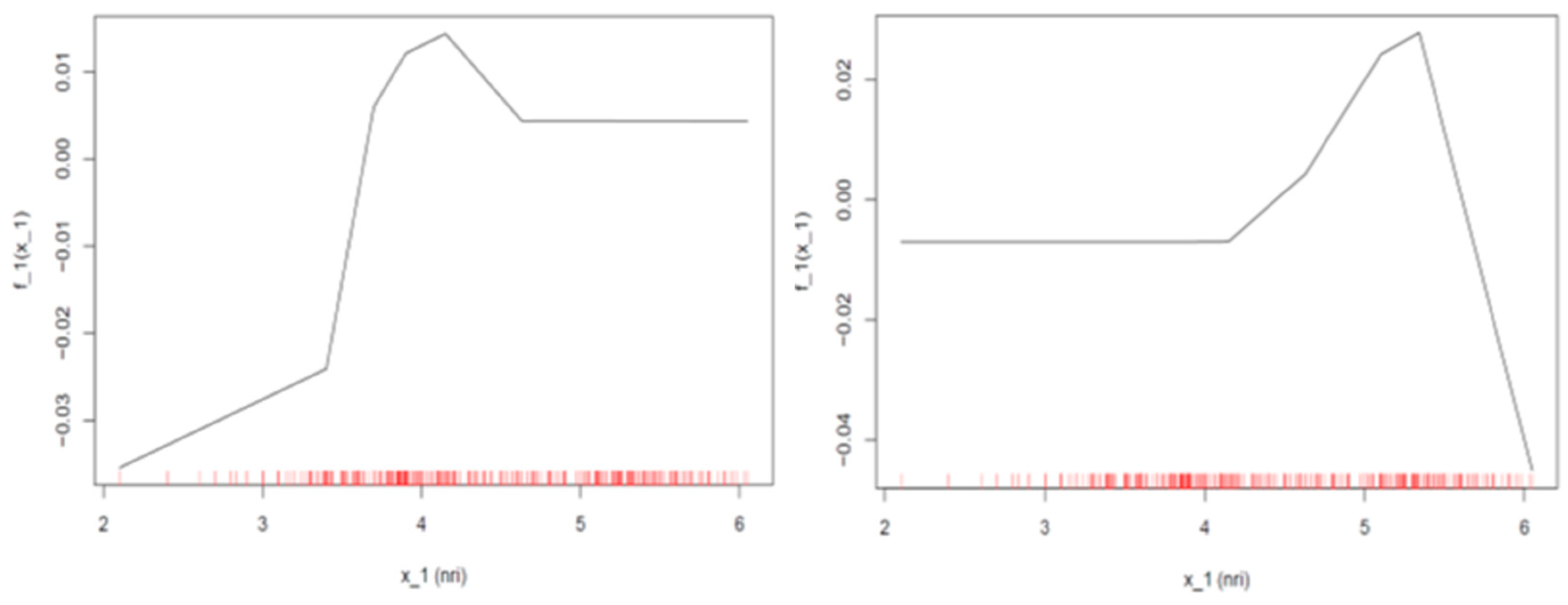
In order to shed some light on the behavior of ICT penetration and the size of the informal sector, we plot their accumulated local effects (ALE) plots, which describe how features influence the predicted outcome on average [
50]. The output here should be interpreted as the vector of the change of predicted probabilities, as the variable of interest varies, one for each response class (20 rating classes in our case).
Therefore, we choose to present the plots only for the assigned ratings equal to (AAA) and (BB+) (first non-investment grade) in order to check the impact of the two predictors at the crucial points when a sovereign spares no effort to be assigned the covetable triple (A) or to avoid being degraded to a non-investment grade (or the contrary).
Concerning the case of the assigned rating is equal to AAA (left plot in
Figure 7), we can see that when the ICT value is below 4.5, a mild negative constant effect equal to 0.005 decreases the probability of being assigned the specific rating, while an improvement of ICT penetration beyond this value raises the probability of being assigned a rating of AAA by about 0.02 with a diminishing trend after the ICT penetration index value surpasses 5.5. Similarly, when the assigned rating equals BB+ (right plot in
Figure 7) and the value of the ICT index is below 4, the effect is negative but diminishes as ICT penetration rises to a magnitude of about 0.01–0.03, and as soon as the index breaches the above limit, the effect becomes positive, reaching a maximum of 0.01 and then falling again.
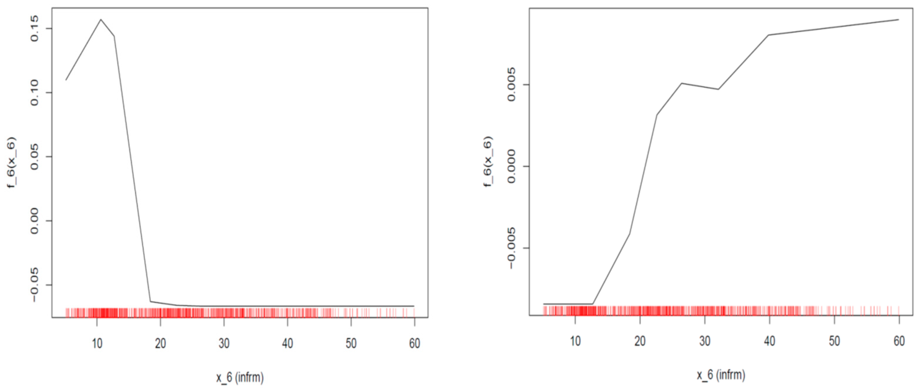
Similarly, concerning the impact of the size of the informal sector when the assigned rating equals AAA (left plot in
Figure 8), we can discern that while the size of the informal sector remains under 10%, it has a positive impact of 0.1 to 0.15 on the probability of being assigned a rating of AAA, but as soon as the size exceeds that limit, the positive impact sharply decreases, and finally, after exceeding the ratio of 15% to GDP, the impact becomes negative.
On the other hand, when the assigned rating equals BB+, the plot (
Figure 8) shows that for the area between values 10–22% of the shadow economy, the impact is slightly negative (−0.005–0.00), but when this limit is surpassed, the impact on the probability of being assigned a BB+ rating steadily increases (0.00–0.01).
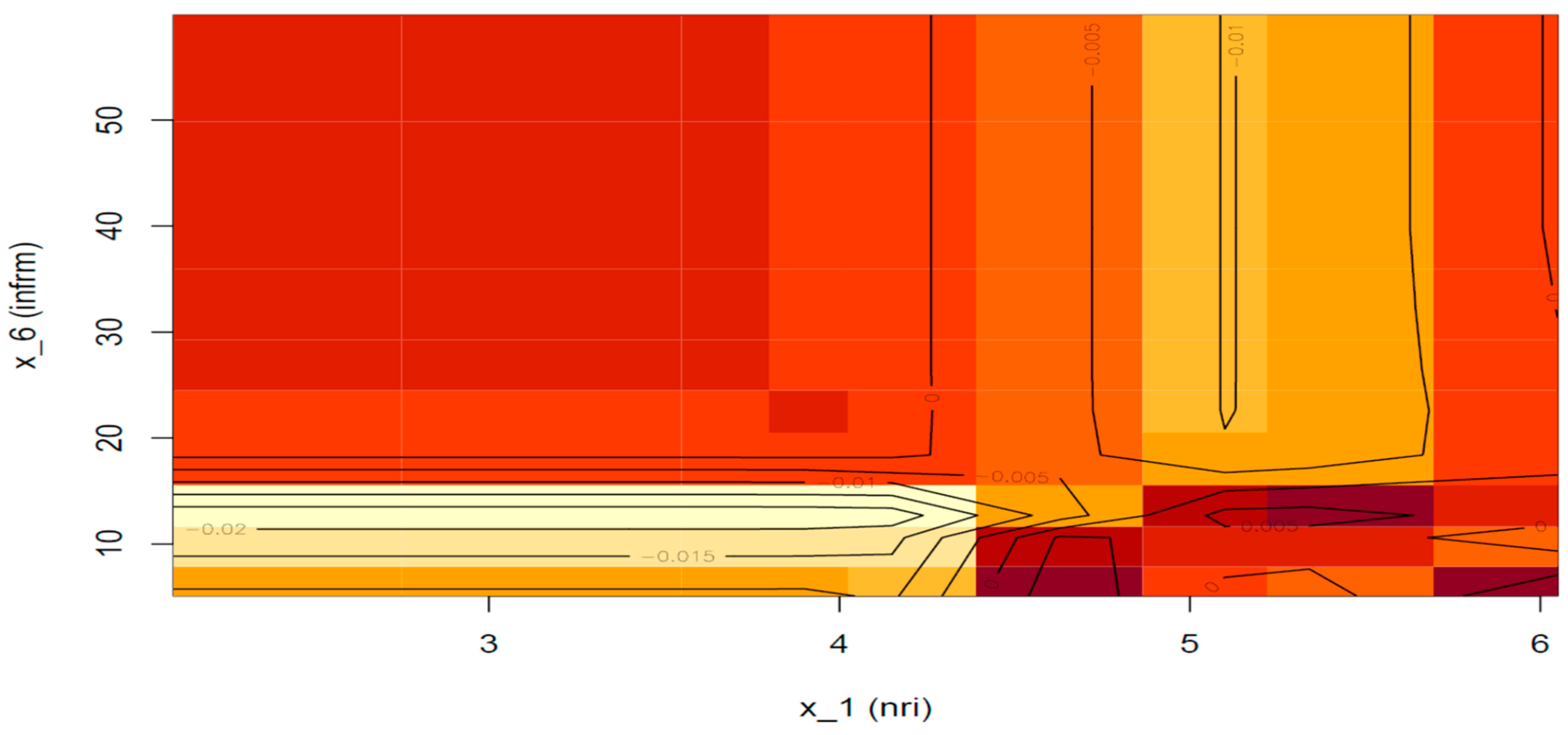
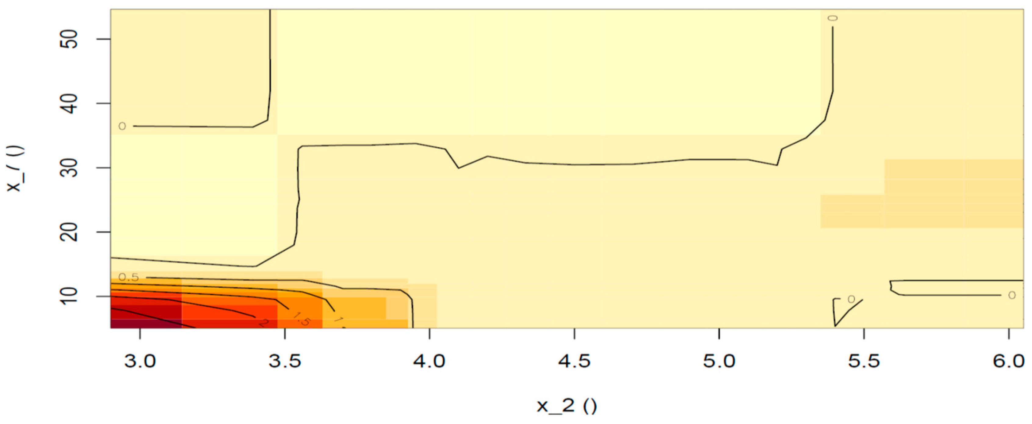
Next, we consider the second-order effect of ICT penetration and the shadow economy (if any) on the prediction (
Figure 9). The area of the plot that is formed when the ICT index is below 4.5 and the informal sector is under 10% will not be considered since the area is far from the data distribution; however, we can see that if the informal sector index ranges between 15–18%, a negative effect of magnitude 0.01–0.02 can be detected, while if the informal sector exceeds 20%, no additional effect is found. Moreover, we can see that if the ICT index is above 4.5 and at the same time the informal sector is confined below 15%, then the interaction of the two determinants adds another 0.005 to the probability of a sovereign being assigned a rating of AAA (lower right part of the plot). Nevertheless, if the informal sector exceeds 15% and the ICT index is larger than 4.5, the additional effect turns negative, with a magnitude ranging from 0.005 to 0.01.
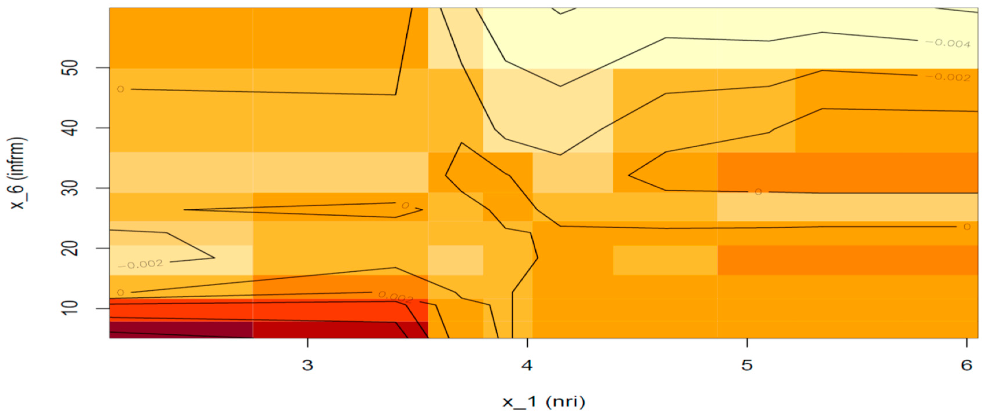
Figure 10 shows the additional net effect of the interaction of the two features when the assigned ratings are equal (BB+), but fails to detect any. Similar to the above, we will abstain from any conclusion driven not only from the red area of the plot but also from the top right area (yellow) because both areas are far from the data distribution.
4.4. Random Forests on Bond Yields
First, we tune a number of hyperparameters in order to adjust them until the validation error stops improving by a certain ratio. Concerning the number of variables randomly sampled as candidates at each split, the optimal number is set to 9 and the number of trees grown to 300; too many trees may lead to overfitting. Our random forest models succeed in reducing the validation error to 2.27 and the testing error to 2.57 (RMSE), while a pseudo-R-squared metric, {1-mse/Var(ytm)} indicates that the variance explained equals 79.03%. Here (
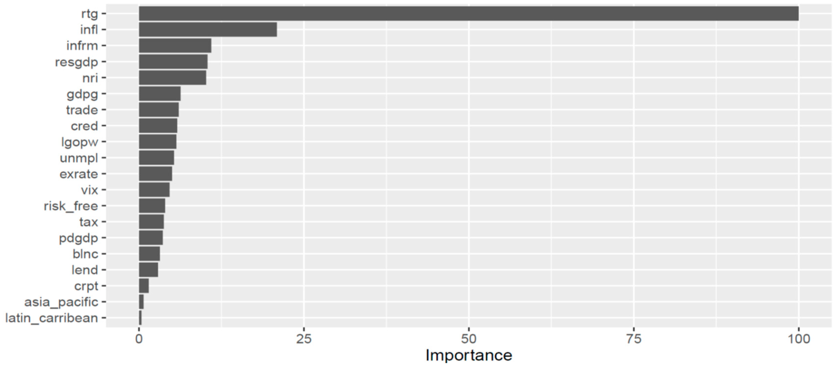
Figure 11) we provide two measures of variable importance after recording the prediction error for each tree: the average difference, normalized by the standard deviation of the differences, between the mean squared error of every validation set with each predictor being permuted and the average total decrease in node impurities from splitting on each variable.
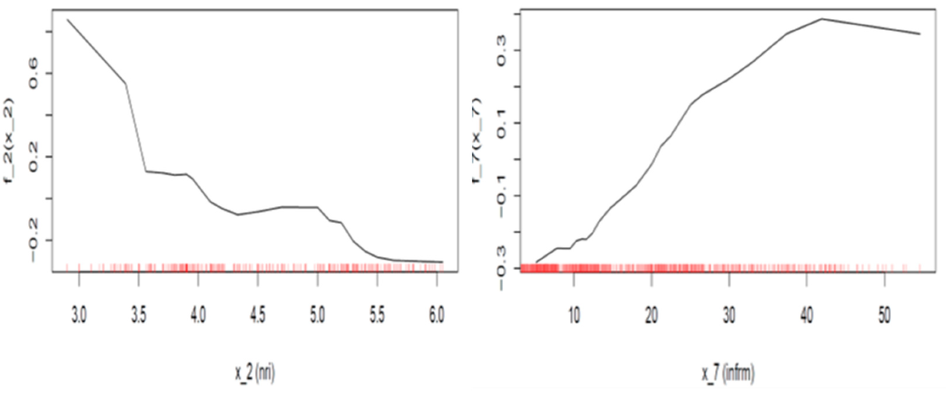
It can be observed that the random forest model takes into account a larger number of determinants in relation to the previous models and considers especially the risk-free rate, credit ratings, trade openness, and inflation. Concerning ICT penetration and the size of the informal economy, they seem to play a modest but considerable role. The accumulated local effects (ALE) plots (
Figure 12) based on the random forest model show that a low rate of ICT penetration (between 3 and 3.5) increases the sovereign yields by around 0.1–0.8 p.p., but with a sharp declining rate and after the variable takes a value of 4.0, no particular effect can be detected on the average prediction. When the variable exceeds the value of 5, then ICT penetration has a negative (decreasing) effect on yields by about 0.2 p.p. On the other hand, a small size of the informal sector has a negative effect on yields of around 0.2 p.p., but a larger informal sector that surpasses a ratio of 20% to GDP has a positive (increasing) impact on yields of about 0.2 p.p. to 0.4 p.p.
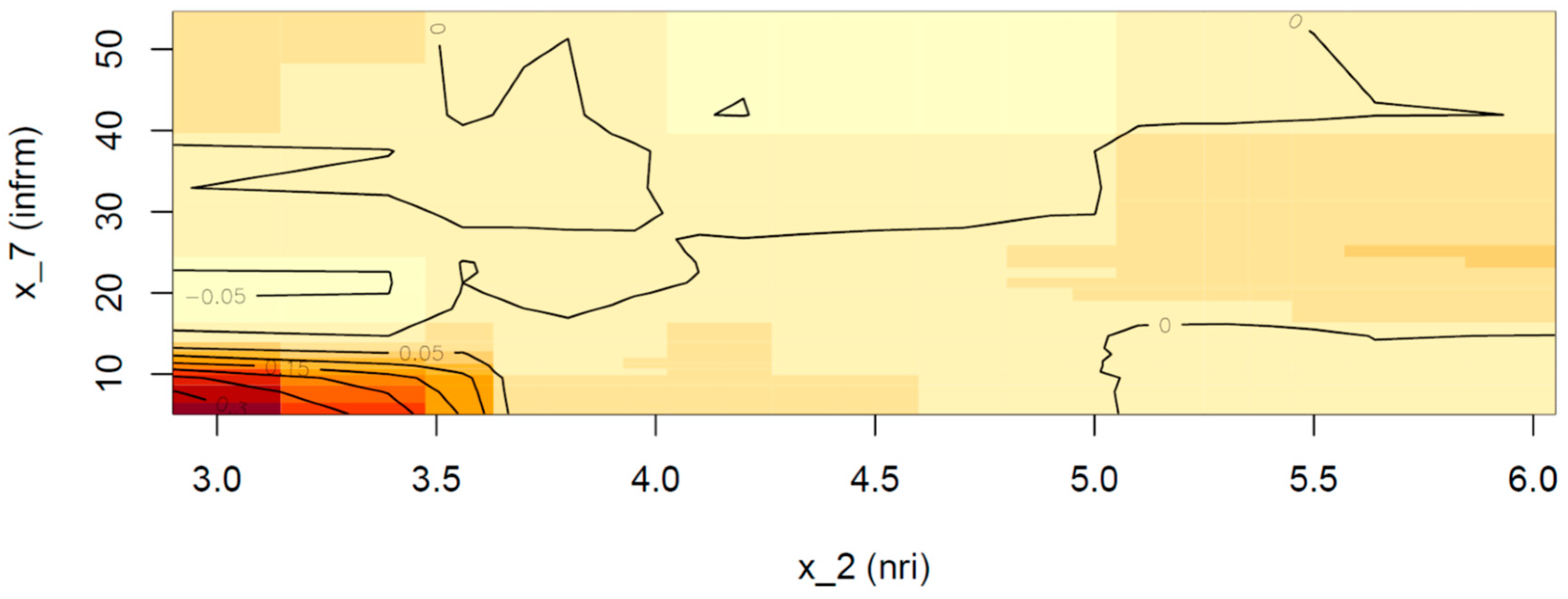
Similarly, the accumulation effect plot (
Figure 13) on the interaction of the ICT penetration and the size of the informal sector shows that an additional negative (decreasing) effect of a magnitude of 0.05 p.p. occurs when ICT penetration is very limited and the informal sector is medium-sized or when the informal sector skyrockets and the ICT penetration is mid-scaled (4.0–5.0).
4.5. Gradient Boosting (We Do Not Present the Gradient Boosting Model for Sovereign Ratings Because It Failed to Deliver a Superior Classification Rate in Relation to the Random Forest Model.)
Instead of creating an ensemble of de-correlated trees such as random forests, gradient boosting builds, in an iterative fashion, an ensemble of shallow and weak trees. A weak classifier (tree) is one whose error is only slightly better than random guessing [
51]. Usually, shallow trees are built with only 1–6 splits [
45].), with each tree being an improvement of the previous since in every iteration the new base-learner is trained on the error learned so far [
45]. The gradient boosting model is tuned by trial and error (a full grid search is computationally expensive in the case of a gradient boosting machine). The learning rate is set to 0.01, the number of iterations to 1040, the tree depth to 15, the minimum number of observations required in each terminal node to 9, the percent of training data to sample for each tree, and the percent of columns to sample for each tree to 80%.
The model further reduces the validation error relating to the previously presented models to 1.38 (RMSE), while the testing error drops as well to 2.41 (RMSE) with an R
2 = 0.73. The variable importance plot (
Figure 14) verifies that ICT penetration and the size of the informal sector are important drivers of the predictions of the gradient boosting model as well. By far, the model places a heavy weight on the assigned credit ratings. Measures of importance are computed based on the fractional contribution of each feature to the model based on the total gain of the corresponding feature’s splits. The ALE plots depicted in
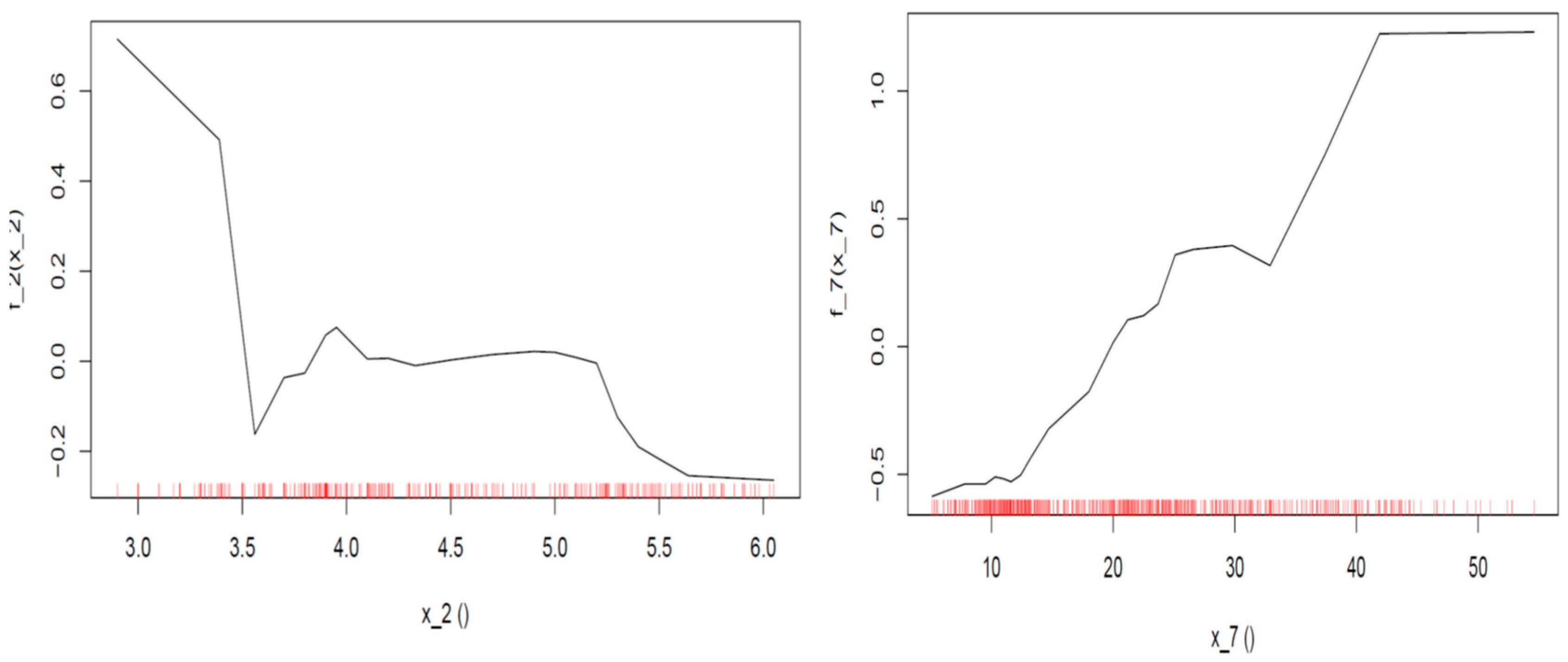
Figure 15 further refine our conclusions. It can be seen that the positive effect of ICT penetration (or better, its lack), when ranging between 3.2 and 3.5, declines rapidly and becomes negative (about 0.2 p.p.) as soon as the feature’s value exceeds 3.5. The plot detects turbulence in the range of 3.5 to 4 since the negative effect is not stable and quickly consolidates around zero until the ICT penetration value exceeds 5. Then the negative effect sharply reaches 0.2 p.p. and seems to stabilize. On the other hand, the negative (decreasing) effect of a very confined informal sector vanishes as soon as the ratio exceeds 20%, corroborating previous results. The effect becomes positive, and afterward, as the slow rate rises slowly, it increases rapidly and stabilizes around 1 p.p.
The accumulation effect plot (
Figure 16) on the interaction of ICT penetration and the size of the informal sector is in line with previous findings and shows that an additional negative (decreasing) effect of a magnitude of 0.25 p.p. occurs when ICT penetration is very low and a medium informal sector accounting for 20–35% is present.
Moreover, a negative effect of the same magnitude (0.25 p.p.) can be seen for levels of ICT penetration between 3.5 and 5.5 in conjunction with a skyrocketing informal sector with a ratio over 40%. The area in red is, again, not taken into account.
5. Robustness Test
Rating agencies have often been accused of a pro-cyclical policy (meaning that rating standards are not consistent over the expansion and recession periods), responding with a considerable lag to shifts in sovereign credibility and therefore not acting as early warning systems to market participants as expected. Moreover, they are allegedly overreacting with abrupt downgrades in times of recession, exacerbating debt crises, remaining very cautious, or underreacting concerning upgrades during recovery phases or even for longer periods. In any case, the strong persistence and high level of inertia that sovereign ratings usually exhibit come as no surprise. The reason for this phenomenon can be traced back to an agency’s reputation mechanism [
52], which seeks to restore their lost reputation due to warning failures by pushing them to excessive conservatism during and after crises. Stickiness may also exist, as it has been argued by agencies [
53] because countries’ economic behavior during crises reveals new (negative) information that was not available beforehand. The conventional econometric approach, when analyzing panel data (datasets where the behavior of entities (countries concerning this study) is observed across time (years in this study)), is to apply fixed or random effects or a complete pooling modeling approach. Nonetheless, given the persistency of sovereign credit ratings, a growing trend in the relative literature is to account for this persistency by applying dynamic panel models [
54], including in the set of independent variables the lags of the dependent. In the models presented in this study so far, we have not accounted for the time-series nature of our data nor for the persistence our dependent variables exhibit.
Considering the above, a machine learning approach, which is gaining recognition lately for efficient handling of such time-dynamic behavior based on recurrent artificial neural networks, is examined further down in this study in order to address the robustness of our findings when tackling these aspects. Moreover, in order to account for any possible irregularities arising from modeling the proxy of sovereign ratings by the standalone S&P ratings, we use as a dependent variable the synthetic measure of the simple average of the three most prominent agencies (S&P, Moody’s, and Fitch;. As a further check for validity, we exclude the synthetic measure of ratings from the set of independent variables of bond yield determinants that are fed to the first layer of the recurrent network to detect the behavior of the remaining features in the absence of a catch-all proxy as ratings.
An artificial neural network (ANN) is a nonlinear model that closely resembles the structure of a biological neural network. Artificial neural networks are made up of layers of nodes, each of which is connected to the others by nonlinear activation functions. Usually, the first layer of an artificial neural network is made up of explanatory variables. The explanatory variables in the middle layer undergo intermediate transformations. The nodes in the final layer are responsible for predicting the dependent variable. Each function is associated with a set of appropriate parameters called weights and biases. Training the neural net entails the optimization of these parameter values by minimizing a loss function that depends on the predicted dependent variable and its true values.
Recurrent neural networks (RNN) [
55,
56] are a special class of neural networks that are utilized in problems where input can be modeled as a temporal sequence. The main purpose of RNNs is to exploit the temporal relationship between input and output in order to improve their prediction accuracy. They have gained particular popularity in the domain of natural language, audio, or video processing and the demand for financial market predictions [
55,
57]. RRNs architecture evolved through the years so as to be able to overcome its initial limitations, such as being able to retain past events in memory for an extended time. Thus, new RNN architectures such as LSTM (long-short-term memory) and GRU (gated recurrent units) are proficient at modeling long-term sequence dependencies. LSTMs sophisticated cell units are able to recognize, “store and preserve” an important input in a long-term state. GRU units accomplish the same performance as the LSTM units but are, in general, faster to train.
In this study, a GRU recurrent neural network architecture has been put to the test with two appropriately prepared datasets. The first dataset consists of 28 features (including all the features plus one used in the previous methods as well as the synthetic measure of credit ratings for 65 countries over a period of 16 years). (Since in all our models we had excluded the risk-free rate as a determinant of the assigned credit ratings, in order to check for potential omitting bias, we included the specific feature in the set of independent variables when feeding the first layer of RNN. Nevertheless, the risk-free rate turns out to be the least important feature with negligible impact (see
Figure 17) and therefore the omission of the variable does not insert any bias into our previous models.) It has been utilized to create a recurrent neural network that predicts the S&P credit ratings based on longitudinal data. Similarly, the second dataset consists of 28 features (including all but one of the features used in the previous methods as well as the bond yield values for 58 countries over periods from 6 to 16 years). (We exclude S&P ratings for the reasons mentioned earlier in the section.) and it has been utilized to create a recurrent neural network that predicts bond yields by exploring past patterns. The two datasets have been appropriately preprocessed. Regarding the credit ratings dataset, each of the 65 countries’ records has been broken into rolling 8-year windows, looking back 7 years to predict the year ahead. Similarly, the dataset concerning bond yields has been broken into rolling 6-year windows. Moreover, the datasets have been further split into training and testing datasets by country to avoid data leakage. The GRU architecture consists of a dense input layer followed by a gated recurrent unit layer, a dropout layer, and a final dense layer. The aforementioned GRU neural network has been implemented utilizing the APIs of Keras, Tensorflow, and the R language. Thus, all hyperparameters have also been tuned with the assistance of Keras Tuner for R. For the credit ratings dataset, the hyperparameters of GRU units, the GRU activation function, the GRU recurrent dropout, the dropout layer rate, and the optimizer learning rate were optimized using Adam, maximizing the accuracy metric (categorical cross entropy) on the validation set utilizing a random search algorithm. For the GRU network used in the bond yield dataset, the same scheme has been used; however, the Adam optimizer has been set to minimize the mean squared error on the validation set.
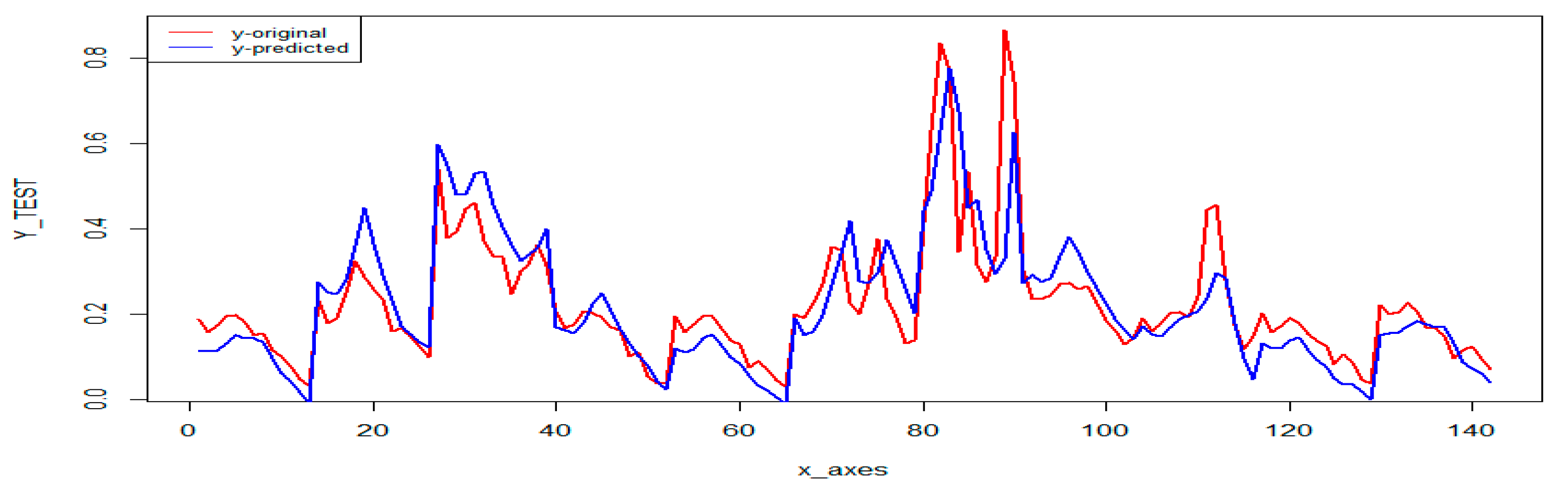
After hypertuning the RNN, the two models have been updated with the new hyperparameter values and then applied to the two datasets. For the bond yield dataset, the RNN performed exceptionally well, presenting an RMSE of 0.0601 on the test set.
Figure 18 presents the original values versus the predicted values by the RNN on the test set. For the credit ratings dataset, the RNN produces a model achieving a more than satisfactory 52.99% accuracy rate on average, which is similar to the best accuracies achieved by our previous models, or 81% if classifying as correct, predictions within one notch of real values. This specification of correct classification has been widely used in the empirical literature due to the difficulty that neural networks present in determining the correct rating in adjacent categories [
58].
Moreover, as Bennell et al. [
44] have suggested, the method is equivalent to artificially creating meta-classes of evenly distributed observations by limiting the number of classification categories, a method that has also been extensively used in the literature (e.g., [
11]).
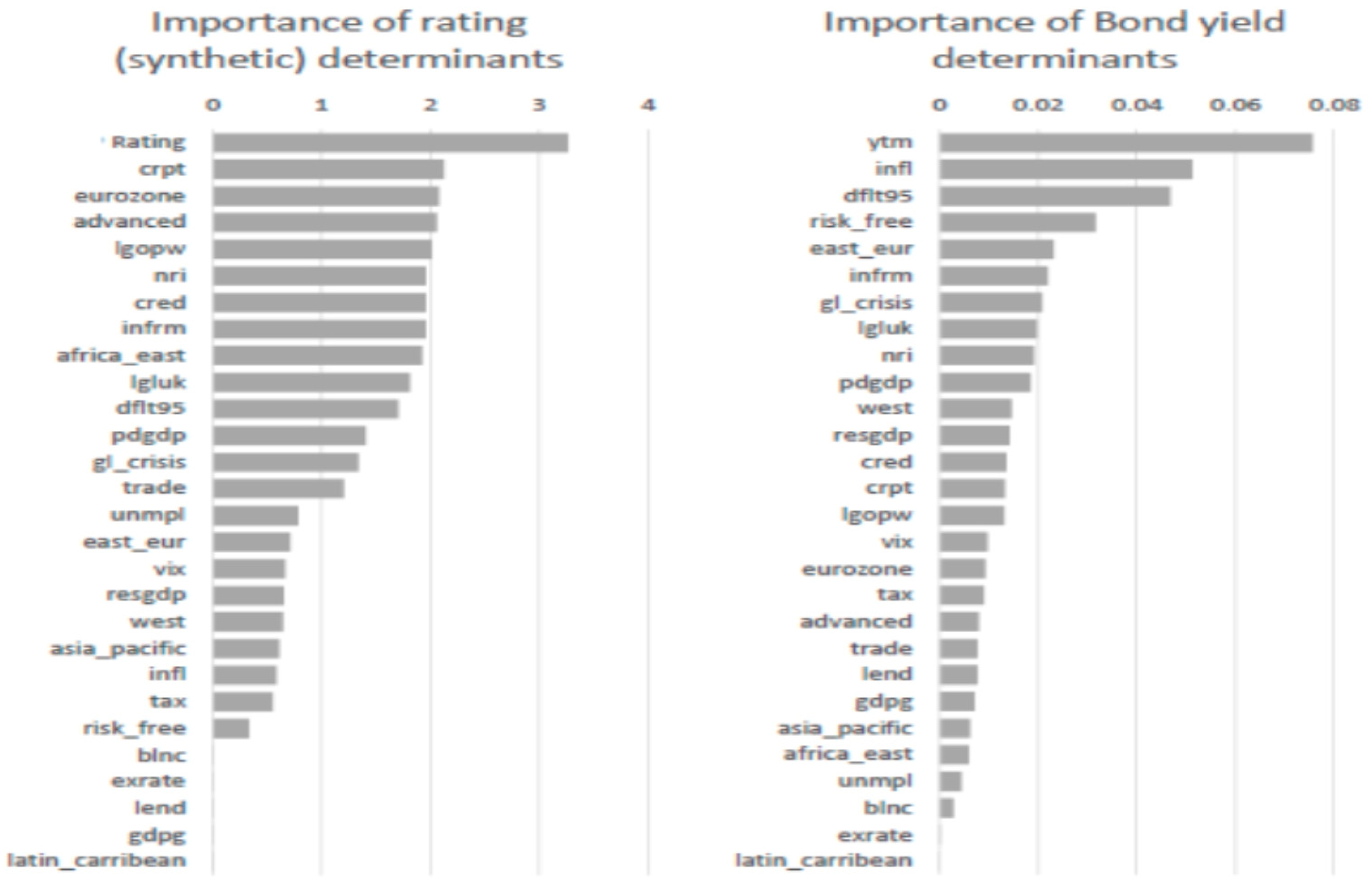
In order to measure the importance of the features for both of the RNN model development, a permutation feature importance technique [
59] has been applied to the test data sets. Next, each variable at a time is shuffled, and the model is utilized again to make new predictions. Afterwards, the root mean square difference between the original prediction and the prediction of the perturbed dataset is calculated. The process is repeated multiple times due to the stochastic nature of the methodologies used. The results of the permutation feature importance technique, presented in
Figure 17, suggest that the ICT penetration rate and the size of the informal sector indeed play a considerable role in predicting risk ratings and sovereign debt rates, despite including lags of the dependent variables in our models or using a different metric as a proxy for the assigned ratings.
6. Discussion
Table 2 presents a summary of the 20 most significant variables obtained by employing different models on credit ratings. We first discuss the variable importance of models that exclude lags in ratings. The three models have a common set of variables in their top rankings, such as worker productivity, the size of the informal sector, and the level of corruption. ICT penetration is also considered important and is ranked sixth by the random forest model after the exchange rate and credit to the private sector. The ratings are expected to be affected by macroeconomic news, which is also observed in the analysis [
60].
The importance of lagged values in our RNN model appears to indicate persistence in credit ratings, as their score is twice as high as that of any other variable. (See
Figure 17). Nevertheless, we cannot officially confirm inertia as conventionally done in the literature by testing if coefficients of lagged variables approach unity [
61]. The levels of perceived corruption and productivity per worker continue to play an important role, along with credit to the private sector, the size of the informal sector, and ICT penetration, which more or less comprise the top-scoring variables. The obvious difference in the RNN model compared to the other three is the high importance of being a member of the eurozone or considered an advanced country, suggesting that these properties are valued by credit agencies beyond the usual information conveyed by the economic fundamentals.
As we have already seen in
Section 3 through ALE plots, when ICT exceeds a value of 4.5, it begins to exert a moderate impact towards a better rating, while when ranging below 4.0, it exhibits an adverse effect.
The plots involving the size of the informal sector suggest that if the ratio ranges between 5 and 15%, the probability of a country attaining the characterization of a high-quality issuer increases significantly by 0.1. Nevertheless, as soon as the size exceeds the critical value of 15%, the effect becomes negative (degrading). The second-order effects detection plots suggest there is an additional small effect of about 0.005 in the probability of being assigned a top rating when the informal sector is detained below 15% and ICT penetration exceeds 4.5. Nevertheless, if, in this case, the shadow economy exceeds 15%, the interaction with a larger informal sector seems to have an adverse effect of around 0.01. Contrary to what was expected, we find no evidence that a larger ICT penetration (meaning above a certain rate) may deter the adverse effects of an expanded shadow economy on ratings.
Concerning yields, a comparison of the variable importance of the different models can be found in
Table 3. The first three models that lack dependent variables lag and identify rather different sets; however, the ratings seem to be appraised by markets as a premium source of information since they are rated as one of the most important determinants after controlling for the economic fundamentals. Moreover, inflation seems to also play the role of an economic indicator and scores systematically high. Furthermore, findings confirm that, apart from country-specific fundamentals, global factors such as the VIX and the U.S. risk-free rate have an effect on debt rates. The informal sector and ICT usage are quite important factors across models, with the size of the shadow economy ranking a bit higher.
The RNN model suggests that, as the most important variable, the lags of the dependent variables have an importance factor that almost doubles relative to any other importance, showing that they also exhibit a rather sticky behavior. The role of inflation and the U.S. risk-free rate seem to be confirmed by the RNN model as well, while some other variables such as the history of defaults, the period of turbulence and economic crisis (2007–2010), and the origin of the law (common law considered safer for investors) seem to gain some importance.
The impact of ICT penetration and the size of the shadow economy are validated by our robustness model but in a more modest direction. The quantification of their impact through ALE plots is quite straightforward since all our models exhibit similar patterns.
When the ICT index ranges between 3.0 and 3.5, the effect is positive and varies from 0.2 to 0.4 p.p., indicating that technological laggards pay a premium. When ICT penetration is moderate (3.5–5), no effect may be discerned, and when referring to ICT pioneers (>5), the negative effect amounts to around 0.2 p.p.
Considering the informal sector when its size does not exceed 20%, a negative (decreasing) effect of around 0.1 to 0.3 p.p. is presented, while when the sector expands, the effect rapidly becomes positive, and when considering skyrocketing (>40%) shadow economies, the effect stabilizes to a rather considerable amount of 1.0 p.p. Concerning the second-order effects, an additional negative (decreasing) effect of a magnitude of 0.25 p.p. occurs when ICT penetration is substantially low (<3.5) in interaction with a medium informal sector accounting for 20–35%. Moreover, a negative effect of the same magnitude (0.25 p.p.) can be seen for a moderate ICT penetration (3.5–5.5) in interaction with a skyrocketing informal sector of a size above 40%. These findings are somewhat in line with our expectations but in a much more intuitive way. It seems that when referring to absolute laggards concerning ICT where governments fail to deliver even the basic services, a medium-sized shadow sector provides some prospects of employment [
23] and income. On the other hand, moderate or even promising ICT penetration in interaction with a large informal sector seems to have a negative impact of about 0.25 p.p. on yields, probably signaling the appraisal of the investors to a government policy that strives to provide its people with all the benefits that a digital economy brings and motivate its citizens to return to (or enter) formality.
7. Conclusions and Policy Implications
The determinants of sovereign credit ratings and the rates paid on sovereign debt are still the subjects of much academic discussion. While economic fundamentals clearly play a significant role, additional factors have been proposed in the literature that could contribute to our understanding of the underlying mechanism. In this study, we introduce two factors that have received less attention but may have a significant impact on the economy and society: ICT penetration as a proxy for digital transformation and the informal sector, which remains part of every economy despite policies designed to eliminate it. In addition, to examine their effect on ratings and the cost of debt, as well as their possible combined effect, we use a series of machine learning techniques and employ state-of-the-art model-agnostic methods such as feature importance and accumulated local effects to better understand the relationships under scrutiny.
Our findings suggest that there is a clear, modest negative effect of ICT diffusion and usage on ratings and rates, with technological laggards paying a premium of 0.2 to 0.4 p.p. and pioneers paying a discount of about 0.2 p.p. Countries with modest ICT penetration do not enjoy any apparent direct effect; nevertheless, if they suffer from a high rate of the shadow economy, their commitment to digitization seems to be appraised by markets at a 0.25 p.p. discount.
In contrast, we discovered a positive relationship between the size of the informal economy and ratings as well as yields. Our research indicates that there is a threshold of approximately 15–20% that is deemed acceptable by both investors and agencies. Countries that manage to keep their shadow economies below this level increase their chances of obtaining a top rating by roughly 0.1. However, if this threshold is exceeded, the informal sector can have an adverse impact. Large shadow economies may be charged a premium of up to 1 percentage point by the markets. Notably, in the presence of poor ICT performance, a medium-sized shadow economy appears to be perceived by investors as a temporary economic safety valve.
Our results are consistent with some studies that suggest that ICT can be a significant determinant of ratings and the cost of debt [
13]. However, we do not find evidence that ICT is the most important factor, as proposed by Bissoondoyal-Bheenick et al. [
10] In addition, we confirmed that a shadow economy can have negative effects on sovereign risk when it exceeds a certain size, around 15–20%, which is in line with the findings of Markellos et al. [
11], who suggested a similar threshold of 18%. Additionally, by presenting evidence that the informal sector of ICT laggards should not be eliminated before advancements in ICT take place, we indirectly support the findings of Ndoya et al. [
62], who suggest that in some cases the underground economy presents a positive economic impact in African countries with low ICT penetration, and therefore a consolidation of ICT infrastructure in these countries could help curb the informal economy by including similar positive economic effects (absorption of unemployed workers, enhancement of entrepreneurial spirit, etc.).
The preceding discussion leads to a few policy implications. Firstly, countries can greatly benefit by keeping their shadow economies below 15–20%, which is the threshold for acceptable rates of informality set by both markets and agencies. Secondly, to take advantage of digitally transformed and interconnected economies, countries must invest heavily in ICT. Finally, if a country has a medium-sized shadow economy and low ICT penetration, it should prioritize improving its digital infrastructure before taking more aggressive measures to tackle the informal sector.


