1. Introduction
History seems to have separated much of chemistry [
1,
2] from the classical theory of fields [
3,
4,
5]. Chemical reactions are found throughout the ionic solutions of biology and chemistry, but they are usually described in a language apparently disjoint from that of classical field theory, even though the reactants and products of chemical reactions are almost always charged and carry significant electrical currents. The reactants, catalysts, and enzymes of chemistry and biology depend on charge interactions for many of their functions.
Field theory has much to offer chemistry, particularly in the study of charged systems, as admirably reviewed in [
6], where the focus is mostly on closed systems. Maxwell’s equations are as universal and precise as any theory and apply to chemical reactions in the plasmas of gases and ionic solutions and liquids in general. Indeed, Maxwell’s equations can be written without any adjustable parameters, implying the universal conservation of the total current [
7,
8]. A theory of the electromechanical response of the charge to the electric field is needed, in that case, to make a complete description of the charged system, i.e., an electromechanical theory of polarization phenomena [
9]. But some properties of the electromagnetic field (e.g., conservation of the total current) are true entirely independent of the electromechanical response. The special systems that are almost completely described by the conservation of the current (without specification of charges) include the electronic circuits of our computers and many properties of the action potential of nerve and muscle fibers. Both systems are almost entirely specified by Kirchhoff’s current law. The question then arises of how we fit chemical reactions into the framework of Kirchhoff’s law and the conservation of the total current, which is remarkably simpler to implement than a full accounting of all the charges in a chemical system.
Here, we show one way to describe chemical reactions in ionic solutions with an extension of classical field theory that does not violate either traditional chemistry or electrodynamic field theory. In this work, we take advantage of the energy variation method [
10,
11,
12], which treats ionic solutions as complex fluids, with interactions, internal stored energy, flow, and dissipation like other complex fluids [
13,
14,
15,
16,
17]. We analyze the open systems through which significant energy, mass, and flows enter and leave the system because such systems are used throughout our technologies. Almost all engineering devices are open. Almost all biological systems are open.
Our analysis begins by defining two functionals for the total energy and dissipation of the system and introducing the kinematic equations based on physical conservation laws. The specific forms of the flux and stress functions in the kinematic equations are obtained by taking the time derivative of the total energy functional and comparing it with the defined dissipation functional. More details of this method can be found in [
11], although most of the systems analyzed there are closed and do not exchange energy, mass, or flux with their environment. We use energy variation methods to link the electric field and reaction dynamics, as done by Wang et al. [
6,
18] for reactions that do not involve charges or electrodynamics and are, for the most part, closed without exchange with the environment.
The generalization to charged open systems allows us to study systems of some importance. Our approach deals with the open electronic devices that can be found in most technologies, including computers. We study the active transporters of biological membranes. These involve charge transport with the environment and do not function, and in that sense do not exist, otherwise. They are open electrical systems.
In a sense, we extend the electrical treatment of the membrane proteins called ‘ion channels’ to deal with transporters. The conservation of the current (in the form of Kirchhoff’s law) provides the crucial coupling between the properties of disjoint sodium and potassium channel proteins that act independently in the atomic and molecular sense because they are well screened. Channels are many Debye lengths apart, shielded from each other by the ions, water dipoles (and quadrupoles), which also contribute to the ionic atmosphere of proteins and lipid bilayers. The atomic-scale function of these proteins is crucial to their biological function. Their coupling is just as important to their function as their structure, but the coupling of these channel proteins is not chemical. The coupling is provided by the cable equation [
19], as biophysicists have called the telegrapher equation versions of Maxwell’s equations (and Kirchhoff’s law), used by Kelvin to design the Atlantic cable [
20] well before Maxwell wrote his equations. The voltage-clamp methods used to study such systems exchange currents and energy with the environment and are, in essence, open electrical systems.
Active transport is one of the most important processes in life. It maintains the concentration gradients and membrane potentials that allow biological cells to function. Indeed, without active transport, animal cells swell, burst, and die. Active transport powers the generation of ATP in both animals (in mitochondria, through oxidative phosphorylation) and plants (in chloroplasts, through photosynthesis). ATP is the currency of chemical energy in all plants and animals, storing in a small organic compound the energy from photosynthesis or oxidation. When hydrolyzed to ADP, the chemical energy is available for the myriad of dissipative processes essential to life. Nearly all of them use ATP as their energy source. Life is complex with many facets. The energy source of life is not.
The coupling of flows in transporters in the inner membrane of mitochondria allows one substance to move uphill (against its gradient of electrochemical potential) using the energy derived from the downhill movement of another substance. Coupling is inherently about the relationships between flows, yet most analyses and simulations of active transporters do not explicitly include a variable for flow. Most do not use the electrodynamic equations for flow, such as the conservation of the total current (Kirchhoff’s law) or a nonlinear version of Ohm’s law. Indeed, most analyses and simulations use methods derived assuming zero flow and do not include changes in potential or free energy associated with the flow. Atomic-scale simulations deal with the myriad of charges in macroscopic systems, like circuits, ionic channels, and transporters, with difficulty. The problems with this approach become apparent if one tries to analyze the electron flow through a resistor, semiconductor diode, or rectifier using traditional chemistry or molecular dynamics approaches.
We analyze an active transporter by studying the currents through it, as a specific example of our general field theory for ionic flows with chemical reactions. We combine Kirchhoff’s law and chemical reaction energetics with the diffusion, migration, and convection of ions and water to make an ’electro-osmotic’ model of a device. The name is chosen to emphasize the important role of electricity in this system, implying the need to deal with electrical flows using methods applied to electrical flows in other systems, like electrical and electronic circuits. This approach seems sensible for systems like oxidative phosphorylation and photosynthesis, where electron flows are involved. The analysis of electron flows has been well established in physics and engineering for more than a century. The analysis of ionic flows has been well established in membrane biophysics for over seventy years. We combine them here with chemical reactions, aiming to construct a useful electro-osmotic theory of cytochrome c oxidase as a device with biologically important inputs and outputs.
We do not have to deal with the myriad of charges involved in the transport of currents or the incalculable number of interactions of those charges that are apparent in the atomic-scale simulations of molecular dynamics. The analysis of the current flow is all we use in this conservative coupling approach, following the practice of circuit analysis. We do not have to assume equilibrium or zero flow. We do not have to deal explicitly with the charges involved in the transport. The analysis of the current flow is all we use. In particular, we do not assume equilibrium or near-equilibrium flows, as done in previous analyses. Note that near-equilibrium analysis (using the Green–Kubo formalism, for example) is inappropriate for devices that function with large flows. These devices are not near equilibrium. The electronic devices of our digital technology function far from equilibrium and they are not analyzed by assuming nearly zero flow. Indeed, they usually use power supplies to maintain spatially nonuniform potentials, often described by inhomogeneous Dirichlet boundary conditions. Traditionally, electronic devices are analyzed by studying small changes around a nonequilibrium operating point, which, we hasten to add, is maintained by large—not small—flows from power supplies. But even this linearization is not necessary nowadays because full-flow nonequilibrium problems can be solved conveniently with readily available software.
We are certainly not the first to exploit the simplification provided by the analysis of a current instead of a charge. Circuit designers have used this approach ’forever’ [
21,
22]. Charges are hardly mentioned when circuits are designed, as a glance at textbooks shows [
23,
24,
25,
26,
27,
28,
29], perhaps most eloquently in symbolic circuit design [
30]. Analyses of currents—not charges—have characterized the study of ion channels since they were discovered as conductances by Hodgkin and Huxley over seventy years ago [
31,
32,
33,
34,
35,
36]. Analyses of currents are not a prominent feature of the study of active transporters; however, even in the work of Hodgkin and collaborators that started the physiological analysis of active transport in cell membranes (in contrast to the study of active transport in biochemical preparations [
37]), at much the same time as Hodgkin led the work defining channels [
38,
39,
40].
Most models of active transport include conformational changes of the protein that require a model to compute the spatial distribution of mass in the protein, as it changes during active transport [
41,
42]. The conformational changes usually provide
alternating access to an occluded state that is not connected (or accessible) to either side of the protein. The occluded state blocks the conduction path (and incidentally, often traps ions in the ‘middle’ of the transporter) and thus prevents backflux. Alternating access mechanisms create flux across the transporter protein without allowing backflux, which would seriously degrade the efficiency of the transporter. Transporters were first thought to use quite different mechanisms from channels [
43,
44]. However, recent work [
45] shows otherwise.
Alternating access is apparently created by correlated motions of gates that account for activation and inactivation in classical voltage-activated sodium channels [
41,
46]. The physical basis of the gates is not discussed in the classical literature. Later in this paper, we speculate that the switches that provide alternating access might be like the switches of bipolar transistors.
In this work, we use an electro-osmotic approach to describe cytochrome c oxidase (or Complex IV) as a device with inputs and outputs, an open system. Our ‘electro-osmotic’ model is a ‘master equation’ approach, building on the work of Hummer and Kim [
47,
48,
49].
We choose cytochrome c oxidase because experimental work and simulations of the highest quality have shown that “cytochrome c oxidase is a remarkable energy transducer (i.e., coupled transporter of electrons and protons) that seems to work almost purely by Coulombic principles without the need for significant protein conformational changes” [
50].
Cytochrome c oxidase depends on an “occluded state” containing the reaction center(s) to prevent backflow, similar to other active transporters, but it uses some type of ’water-gate’ mechanism, as proposed in [
50,
51]. The alternating access in cytochrome c oxidase occurs without a conformation change (of the spatial distribution of mass) in marked contrast to the usual alternating access models of transporters. Perhaps the gate in the oxidase is like the switch in a semiconductor (diode) rectifier. The switches might be rectifiers produced by spatial distributions of permanent charges, or of opposite signs, as rectification (and switching) is produced in PN diodes and bipolar transistors. Diode rectifiers depend on changes in the shape (i.e., conformation) of the electric field, not changes in the distribution (i.e., conformation) of mass. This idea is outlined in
Section 5 following [
52,
53,
54].
The rest of this paper is organized as follows. In
Section 2, we derive the general three-dimensional field equations for an ionic system with reactions and use them to create a general framework of an electro-osmotic model. In
Section 3, we propose a specific, simplified model for cytochrome c oxidase. In
Section 4, we carry out computational studies of our cytochrome c oxidase model and explore the effects of various conditions on the transport of protons across the mitochondrial membrane. In
Section 5, we conclude our paper with a discussion of our cytochrome c oxidase model and future directions.
2. Derivation of Electro-Osmotic Model
We mainly focus on a mathematical model of elementary reactions
where
and
are two constants for forward and reverse directions, and
is the concentration of the
species. Here,
is the stoichiometric coefficient, and
is the valence of the
species, and together, they satisfy
In particular, we have in mind a case where an active transporter (‘pump’) uses the energy supplied by a chemical reaction to pump molecules. Later, we focus on the reaction for cytochrome c oxidase, i.e., Complex IV of the respiratory chain
According to the conservation laws, we have the following conservation of chemical elements (like sodium, potassium, and chloride). Note that this conservation is in addition to the conservation of mass because nuclear reactions that change one element into another are prohibited in our treatment, as in laboratories and most of life.
In order to derive a thermal dynamically consistent model, the energy variation method [
11] is used. Based on the laws of the conservation of elements and Maxwell’s equations, we have the following kinematic system
where
are the passive fluxes,
is the pump flux, and
is the reaction rate function. All these variables are unknown and will be derived using the energy variation method.
is the flux of electrons supplied from an external source. In mitochondrial membranes, this flux includes special structures and pathways linking one enzyme and one complex to another through the movement of lipid-soluble or water-soluble molecules like quinones, which act as electron donors, or acceptors linking one respiratory complex with another, for example.
is Maxwell’s electrical displacement field, and with electric field , dielectric constant , and relative dielectric constant . The equation implies that there exists a such that . We consider a system with structure and boundary conditions defined based on that structure.
The structures are given to us by structural biologists reporting the work of evolution. The structures are complex, as complex as the structures of integrated circuits and modules of circuits in our computers. But the structures are known, often in quantitative detail, thanks to the work of generations of anatomists and histologists. Thus, they provide fewer adjustable parameters than one might imagine if one were not familiar with the work of structural and anatomical biologists.
The structures are decorated with molecules (proteins and lipids for the most part) that use particular atomic arrangements to channel physical forces into physiological functions. The physiological properties of these proteins (channels and transporters) are known in great detail and have few adjustable parameters because of the work of generations of membrane biologists and electrophysiologists.
Channels can be studied one molecule at a time in their natural environment, and the atomic detail structures are known in many cases thanks to the heroic work of structural and molecular biologists. The work of generations of quantitative biophysicists means that there are fewer adjustable parameters in our models than might seem to those unfamiliar with this biological work.
We describe the flux for the
species
, which serves as the input of the system. In cytochrome c oxidase, the input is electrons carried on the heme groups of cytochrome oxidase.
We use the assumption that polarization can be described by a single positive constant called the dielectric constant
because in many cases, too little is known to do anything better. When more is known experimentally, the dielectric description of polarization needs to be replaced with an electromechanical description of polarization as a stress–strain relation of lipid-soluble or water-soluble electron donors, with a slightly modified version of Maxwell’s equations, as discussed in [
55,
56] from various perspectives.
Remark 1. By multiplying on both sides of the first three equations and on both sides of the fourth equation, we havewhich is consistent with the electrostatic Maxwell’s equations. The treatment of transient problems involving displacement currents is needed to deal with some important experimental work [57,58,59,60,61,62]. The total energetic functional is defined as the summation of the entropies of mixing [
63], internal energy, and electrostatic energy.
Then, the chemical potentials can be calculated from the variation in total energy
It is assumed in the present work that the dissipation of the system energy is due to passive diffusion, chemical reactions, and the pump. Accordingly, the total dissipation functional
is defined as follows
where
is the term for the pump.
Open systems in which some fluxes flow in or out, entering or leaving the system altogether, have distinctive energy dissipation laws that differ from those of closed systems. The natural mitochondrion is an unclamped system, in which the electrical potential assumes whatever value satisfies the field equations. The sum of all currents across the membrane of the natural mitochondrion is zero (including the capacitive displacement current), as it is in small biological cells. Many experiments are conducted on voltage-clamped systems. In these, the sum of the currents does not equal zero, just as the sum of the currents in the classical Hodgkin–Huxley experiments was not zero. Of course, the ratio of fluxes will be different in the clamped and unclamped cases, as we document at length later in this paper.
In the natural unclamped mitochondrion, we have the following generalized energy dissipation law
where
is the rate of boundary energy absorption or release that measures the energy of flows that enter or leave the system through the boundary. Recall that the chemical potential of a species is the energy that can be absorbed or released due to a change in the number of particles of the given species, and
is the total number of the
particles passing through the boundary per area per unit time. We define
as follows
In general, different types of boundary conditions can be written in the following general format
where
is the conductance of the
species on the boundary,
is the fixed reservoir’s concentration of the
species, and
f is some specific function. Then, the rate of boundary energy absorption or release is
In this open case, characteristic of electronic devices, ion channels, and transporters, energy can change because of both the flux across the boundary and the change in dissipation.
Remark 2. Boundary Conditions, Structure, Evolution, and Engineers
These boundary conditions serve as the link between general field equations and structures that serve as devices. Structures are chosen and devices are designed (by evolution or engineers) so these boundary conditions are satisfied. The boundary conditions are chosen so devices have almost the same properties no matter where they are placed in a network. The structures and boundary conditions of those structures are not automatic properties of nature. The structures are decorated with (i.e., include) specific substructures (like power transistors) that exploit arrangements of atoms (like doping charges) to create properties that are useful. The properties are summarized by boundary conditions located on the structures provided by evolution and engineers. These boundary conditions help make the idea of a component useful. They help ensure that a component in one part of a system does the same as what it does in another part of the system; therefore, they can be described by a ‘transfer function’, independent of the component’s location in the system. The transfer function can be analyzed by the currents that flow through it, with almost no attention to the charges that make up that flow, as a glance at circuit textbooks shows [23,24,25,26,27,28,29], perhaps most eloquently, in symbolic circuit design [30]. It is clear that channels and transporters in biological systems behave as components and often as devices. It seems likely that an analysis of the currents through these components will be as helpful as it is in an analysis of circuits, not requiring an analysis of charges and their individual behavior. Indeed, classical physiology and biophysics are frequently devoted to identifying such components, on a wide variety of length scales from atoms to organisms, and studying how they interact in the hierarchy of the structures of animals and plants [64,65,66,67,68,69,70,71]. Remark 3. - 1.
A closed system allows no flux across the boundaries. It has the following no-flux boundary conditions In a closed system, , and the energy dissipation law is In a closed system, the energy changes into dissipation. This is the only way energy can change in a closed system.
- 2.
An open system has flows across the boundaries. An open system might have constant inflows/outflows - 3.
For the Dirichlet boundary condition on , the flux is unknown and part of the solution. In this case, is the unknown flux that is needed to ensure that the Dirichlet condition is obeyed on . In biophysical language, is the ‘current’ supplied by the voltage-clamp amplifier that is needed to keep the voltage constant, as membrane conductance varies.
It is very important to understand this requirement. In reality, i.e., in experiments and their models, supplying the unknown flux requires specialized instrumentation, for example, a patch clamp amplifier in a voltage-clamp setup. Almost always, this flux is supplied at one location in space. In this way, a classical voltage clamp can be established. One can clamp the voltage in this way but one cannot clamp a field in this way. A voltage clamp is possible, but a constant field is so much more difficult that it is practically impossible.
If one wishes to “clamp” a field, one must control the potential at many locations. Each location requires a different flux and thus a different amplifier and different electrodes to supply that flux. Without such a complicated apparatus, it is almost impossible to maintain a constant field in space [72]. Indeed, it is nearly impossible to maintain any pre-specified field because it is practically impossible to apply different fluxes at different locations. If one assumes a constant field in a theory, without such an apparatus in an experiment, one is, in effect, introducing a flux into the calculation and model that is not present in the experimental setup. One is introducing an artifactual flux likely to produce artifactual conclusions that are not relevant to the original experiment. [54,73]. To indulge in slight hyperbole, one can clamp the voltage, but one cannot make a constant field.
By taking the time derivative of the total energy function (
10), we have
where
and Equation (
2) is used.
By comparing this with the dissipation function, we have
And the corresponding energy influx rate is
For the pump flux, if we assume the flux is only along the
z-direction, then,
The last equation means that
According to the definition of the equilibrium constant
[
74],
Substituting Equation (
24) into Equation (
23) yields
with
Then, combining Equations (20b) and (
25) yields
which implies that
where
[
18].
Remark 4. Here, is dimensionless. and have units of [74]. Then, the whole system is as follows
with
and the boundary conditions
Remark 5. If we assume that one of the reactants is an electron, for instance, , and is supplied by a thin electrode along the z-direction, the density of electron . Then, the model is changed to Remark 6. When the reaction and ions are in an electrolyte, the fluid effect needs to be taken into consideration. In this case, the energy function is changed toand the dissipation function is changed towhereand is the velocity. We can use the energy variation method to obtain the diffusion–reaction–convection model as follows Note that here, we are not considering transient problems in which the charge is stored in polarization fields. These will be studied separately so we can deal with the important experiments reported in [
57,
58,
59,
60,
61,
62]. Transient problems are obviously important if reactions are studied on the atomic scales of distance and time (angstroms and femtoseconds) because the polarization currents are large. Dealing with these currents requires the use of a universal form of Maxwell’s equations combined with an appropriate model of the stress–strain relation of a charge in a viscoelastic structure, commonly called polarization. Speaking loosely, the transient problems can be dealt with in circuits using a generalization of Kirchhoff’s law [
7,
75] to describe the actual transient currents that flow through an ideal resistor [
55].
It is important to realize that currents (and fluxes) cannot be computed using methods that assume currents and fluxes are zero. Electrostatics cannot compute currents because currents and fluxes involve time and electrostatics does not [
76]. Electrostatics does not include Ampere’s law, which is the universal coupler of a current to electric and magnetic fields. In the context of cytochrome c oxidase, these issues come to the fore. Models without electron or proton currents as variables do not describe the ‘transfer function’ of the transporter being studied. Models cannot calculate Ohm’s law (for systems with large and small currents and electrical potentials) if the models assume currents are zero.
In fact, using a formulation of electrodynamics that explicitly involves currents is straightforward, as engineers have known for a very long time, going back to the work of Heaviside [
77,
78], and is worked out in practical detail in [
75]. Kirchhoff’s current law allows for the analysis of systems of great importance, without dealing with charges explicitly. This is why the analysis of electronic circuits does not need to use distributions of charges but rather uses Kirchhoff’s current law or its generalization, the conservation of the total current. Kirchhoff’s current law is an exact corollary of Maxwell’s equations themselves if the current includes the displacement current [
7,
55,
75].
It might seem that another corollary of Maxwell’s equations, the continuity equation, can be used instead of Kirchhoff’s law for the total current. And it is certainly true that the continuity equation of electrodynamics contains the same information as the conservation of the (total) current, all conjoined with Maxwell’s equations. But that information is not useful when enormous numbers of charges are involved, as in cytochrome c oxidase or other macroscopic-scale systems like the electronic circuits of our computers, ionic channels, or transporters in general. Indeed, enzymes, in general, are often macroscopic systems when one considers the environment that is absolutely required for them to function biologically.
The information implicit in the flux of charges is only usable when written as the total current that is conserved perfectly whenever Maxwell’s equations are valid. This formulation using the conservation of the total current does not require the explicit treatment of charges. The continuity equation does require the explicit treatment of charges and their significant interactions, whether involving the interactions between two charges, three charges, or the interactions of an entire cluster expansion. The significant interactions of charges are difficult to understand or even enumerate and more difficult to compute [
79,
80]. Kirchhoff’s current law is easy to understand and trivial to compute.
3. An Electro-Osmotic Model of Cytochrome c Oxidase
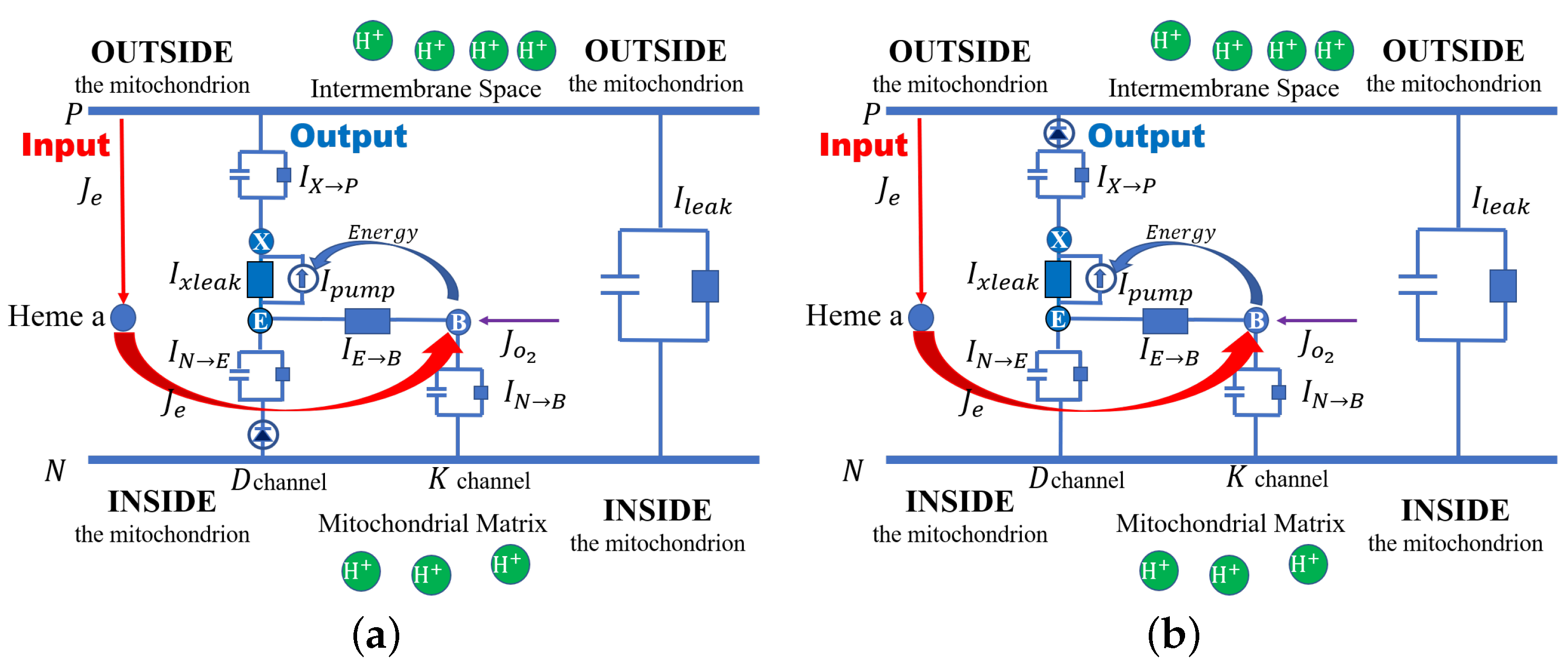
Here, we propose a specific model of cytochrome c oxidase (or Complex IV) as an example so our approach to electrochemical open systems can be seen in action. The schematic structure of cytochrome c is shown in
Figure 1, where both channels from the mitochondria matrix (inside), D and K, are taken into consideration. Here,
E denotes the end of the
D channel. The end of the K channel is assumed to be the binuclear center (BNC), denoted by
B, where the chemical reaction (
36) occurs. The protons accumulated in E are transported to the BNC and the proton loading site (PLS), denoted by X. A pump is located between E and PLS. The pump provides the energy that comes from concentration gradients, namely the gradients of the chemical potential at the BNC. Then finally, the proton is pushed out from the PLS to the inter-membrane space outside the mitochondrion.
It is clear that this model is incomplete at best, and in some sense, wrong at worst. We depend on our experimental colleagues to help us correct and improve the model, for example, by including mechanisms we have oversimplified. Significant details about the chemical reactions are described in the literature, with more intermediates being reported frequently. We do not include these intermediates because we do not know which ones are important for the resolution of the understanding we seek here.
Let
. Integrating the diffusion-reaction equation
with the Complex IV compartment yields
where
,
, and
are the volumes of the mitochondrial compartment, inter-membrane space, and reaction compartment, respectively.
The chemical reaction in the cytochrome c oxidase (Complex IV) is
For simplicity, we follow the Hodgkin–Huxley tradition and fix the proton concentrations in the mitochondrial matrix (inside) and the inter-membrane space outside the mitochondria so they do not vary with time or flow. More general treatments in which concentrations are changed with time by flow are possible, as performed in even more complex structures. Such analyses have been conducted in a bi-domain model of the lens of the eye and a tri-domain model of the optic nerve and glia [
81,
82,
83,
84].
Here, for simplicity, we assume that the concentration of oxygen at the B site is constant. If the oxygen varies with time, an additional equation can be used to describe the dynamics of oxygen. The properties of this term can be determined either directly through experimentation or with the use of a higher-resolution model, as in [
85]. We do not expect the extra term to introduce significant mathematical, numerical, or computational difficulties.
Many variables are needed to keep track of all the potentials and concentrations in the various regions of our model. The variables are required whenever practical systems are described, whether the systems are devices of engineering or creations of evolution. They cannot be avoided in a useful analysis of a functioning system because the parameters describe the conditions needed to make the device or system perform its function.
The concentrations and potentials at
; the BNC; and the proton loading site (PLS) are different inside and outside the mitochondria, as is the electron concentration. They are described by the variables
,
,
,
,
,
,
,
, and
, respectively.
with the currents
We follow the review of Wikström [
50] and implement switching functions without invoking conformation changes in the distribution of mass. We treat cytochrome c oxidase as a Coulomb system and use rectifiers to implement the switching functions that provide alternating access to an occluded state.
Here, we discuss two cases. In one case, a rectifier between N and E blocks the proton flows. In the other case, a rectifier between X and P blocks the backward proton flows. Then, the currents and are modeled in the following two cases.
Case 1: the rectifier is between
N and
E, as shown in
Figure 1a
Case 2: the rectifier is between
X and the outside, as shown in
Figure 1b
where is the threshold for the turn-off of the rectifier, and stands for the perfect rectifier. We reiterate that PN junctions are used to rectify the movement of pseudo-ions’ holes and electrons throughout our digital circuitry. Analogous distributions of permanent charge provided by acid and base side chains of proteins produce a rectification of the charge movement in ionic systems.
We use Kirchhoff’s law and the conductance formulation of Hodgkin and Huxley. Complex properties are hidden through a nonlinear, time-dependent version of Ohm’s law and modeled using conductance, as demonstrated by Hodgkin and Huxley [
31,
32,
33,
34,
35,
36]. Alternating access (with its implied occluded state) is described by a switching function for the D channel using Equation (
39a). This is a classical rectifier function, and when
, it allows for the current only to flow from D to E; no backward flow is allowed.
Many properties of the model depend on the pump current between and the PLS. We assume that in an ordinary case, the pump strength depends on the reaction rate and the chemical reaction difference between the two sites. However, in a less ordinary case, when the difference is too large, the pump may not be able to overcome the barrier. A turn-off threshold is assigned to the pump for this reason. We assume that when the difference in chemical potential is greater than the threshold, the pump current decreases exponentially to zero as it turns off. More realistic and complex properties of the pump will undoubtedly be needed to explain some functions of cytochrome c oxidase. They can easily be incorporated into our model, as these properties are measured and modeled.
What we propose here is in the tradition of Hodgkin’s treatment of ionic channels, but we include the chemical reactions that are the essence of oxidative phosphorylation and the life and function of mitochondria. We are more than aware that a detailed analysis of alternating access, the occluded states, and the switching function is needed to understand cytochrome c oxidase, which requires an analysis of the currents flowing along with the atomic detail of the water-gate switch [
50,
51], in our view. The switches act on currents and, of course, satisfy the conservation of the current. An analysis of charges cannot easily guarantee the conservation of the current, and classical chemical analyses preclude large currents because assuming equilibrium or near-equilibrium conditions is clearly inappropriate for a system like Reaction Center IV, which is designed for the efficient handling of large flows of electrons and protons. Here, we describe alternating access with the classical equation of a rectifier to highlight the possibility that occluded states and alternating access are the biochemical names for what engineers call rectification.
It is important to realize that rectification is an automatic unavoidable consequence of the distribution of doping in semiconductors, for example, in the classical PN diode. This rectification occurs with no change in the spatial distribution of mass (i.e., with no change in what is usually called conformation), and so it is compatible with the view cited above that cytochrome c oxidase functions without changes in the spatial distribution of mass, i.e., without what is classically called a conformation change. In the rectification mechanism, the switching (rectification) occurs because of a radical change in the distribution of the electrical potential, which, in turn, allows current flow in one direction but not another. The distribution of potential depends on the distribution of mobile electrons, which have almost no mass. The conformation of the potential profile, and thus the electric field, creates a barrier for current flow in one direction but not another because of the effects of doping (permanent charge) and mobile charge combined in the Maxwell–Gauss law or the Poisson equation. This system is rather complex, although completely understood and used in billions of different places in our computers. The system involves the diffusive and electrical movements of electrons (and holes) driven by the gradients of the chemical potential (e.g., concentration) and electrical potential. As the electrical potential changes sign, diffusive and electrical flows change. As concentrations change, diffusive and electrical flows change in other ways. All interact through the changing fields of both the electrical and chemical potentials. Over ten pages (not just a few words or sentences) are needed to explain how each kind of movement (diffusive, electrical, holes, and electrons) contributes to rectification because each movement has distinct driving forces that can be varied independently in experimental and technological situations, and of course, each movement is also driven by the other driving forces to which it is coupled (see textbooks on semiconductor circuit design, e.g., [
86,
87]). It is also important to consult research articles [
88,
89] to understand the oversimplifications of the textbook discussions and validate them. More elaborate patterns of doping, starting with PNPN designs (thyristors, Silicon-Controlled Rectifiers (SCRs)) are used in power transistors. Analogous spatial distributions of permanent charge (and acid and base side chains) might be used to implement switches in cytochrome c oxidase.
We note that rectification arising from the distribution of the permanent charge in a protein was proposed by Mauro a very long time ago [
90,
91] as a natural generalization of Shockley’s work on hole and electron conduction in semiconductors. Such rectifiers of ionic currents have even more complex properties than semiconductor rectifiers because concentrations of current carriers in biological solutions can be changed independently of the electrical potential, which is not often the case in analogous semiconductor systems.
This theoretical work can be implemented in practical devices. Ionic rectifiers were built a long time ago using a biological protein as a template [
53] and are now used routinely in the ionic channels of nanotechnology [
92], even in a hybrid chip that can enable a scalable integrated ionic circuit platform for micro-total analytical systems [
93].
The switch of Reaction Complex IV is likely to involve both the distribution of the permanent charge (mostly acid and base side chains) and the chemical interactions, as described in the water-gate model [
50,
51], perhaps also involving the spatial distribution of the dielectric properties [
94]. It seems premature to attack this problem here, as important as it is for the function of cytochrome c oxidase, and all alternating access transporters for that matter. Here, we simply describe the rectification without further analysis of how it arises from the distribution of the permanent charge and other properties in the transporter structure.
Of course, other possibilities exist. Alternating access might arise, for example, from bubbles in the conduction pathway, which we are studying in another work [
95]. Two bubbles might act as coupled activation and inactivation gates, correlated to provide alternating access to an occluded state, for example.
4. Results
In this section, we carry out several computational studies to explore the effects of various conditions on proton transport efficiency. The initial values and default parameters are listed in
Table 1 and
Table 2.
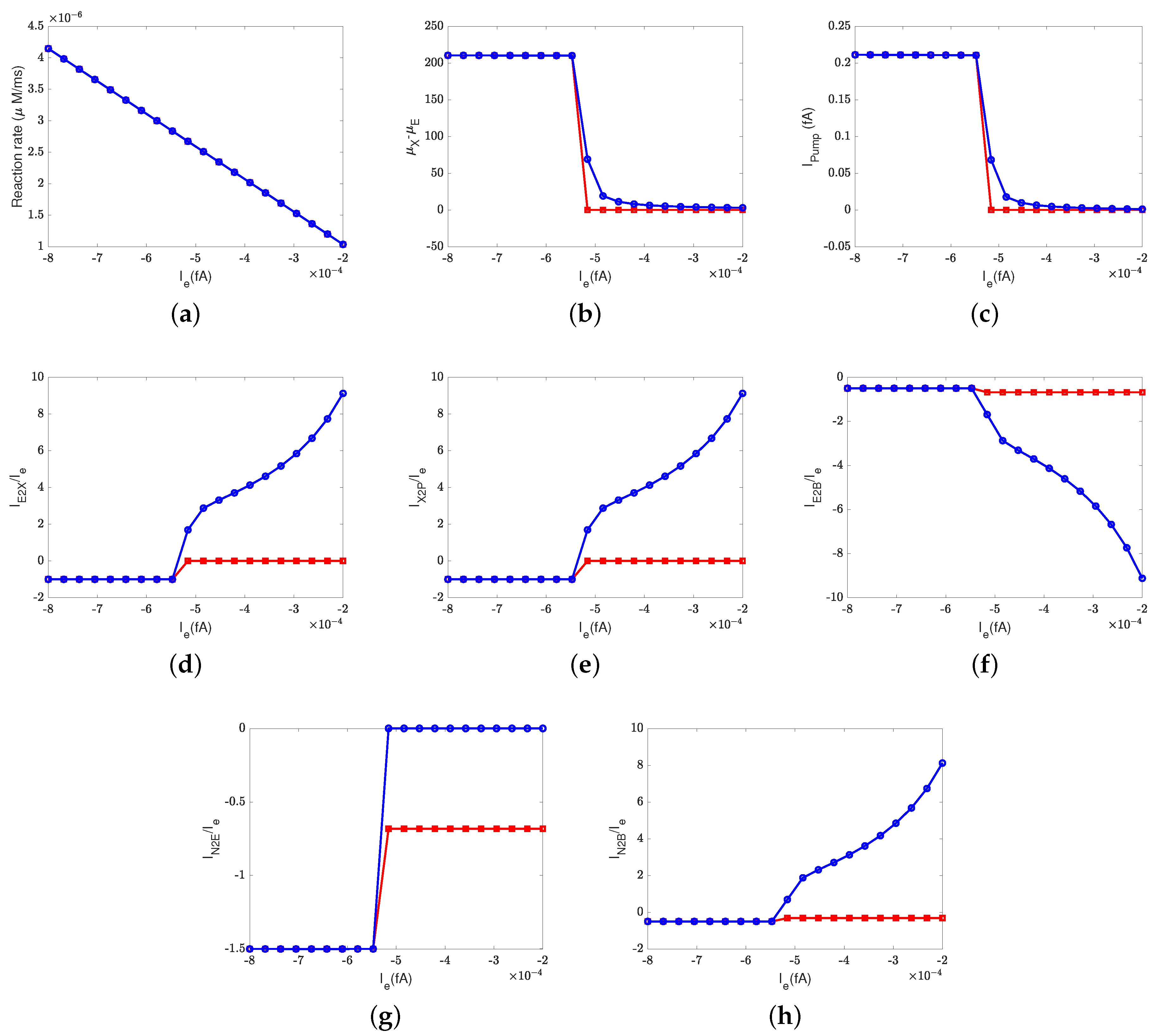
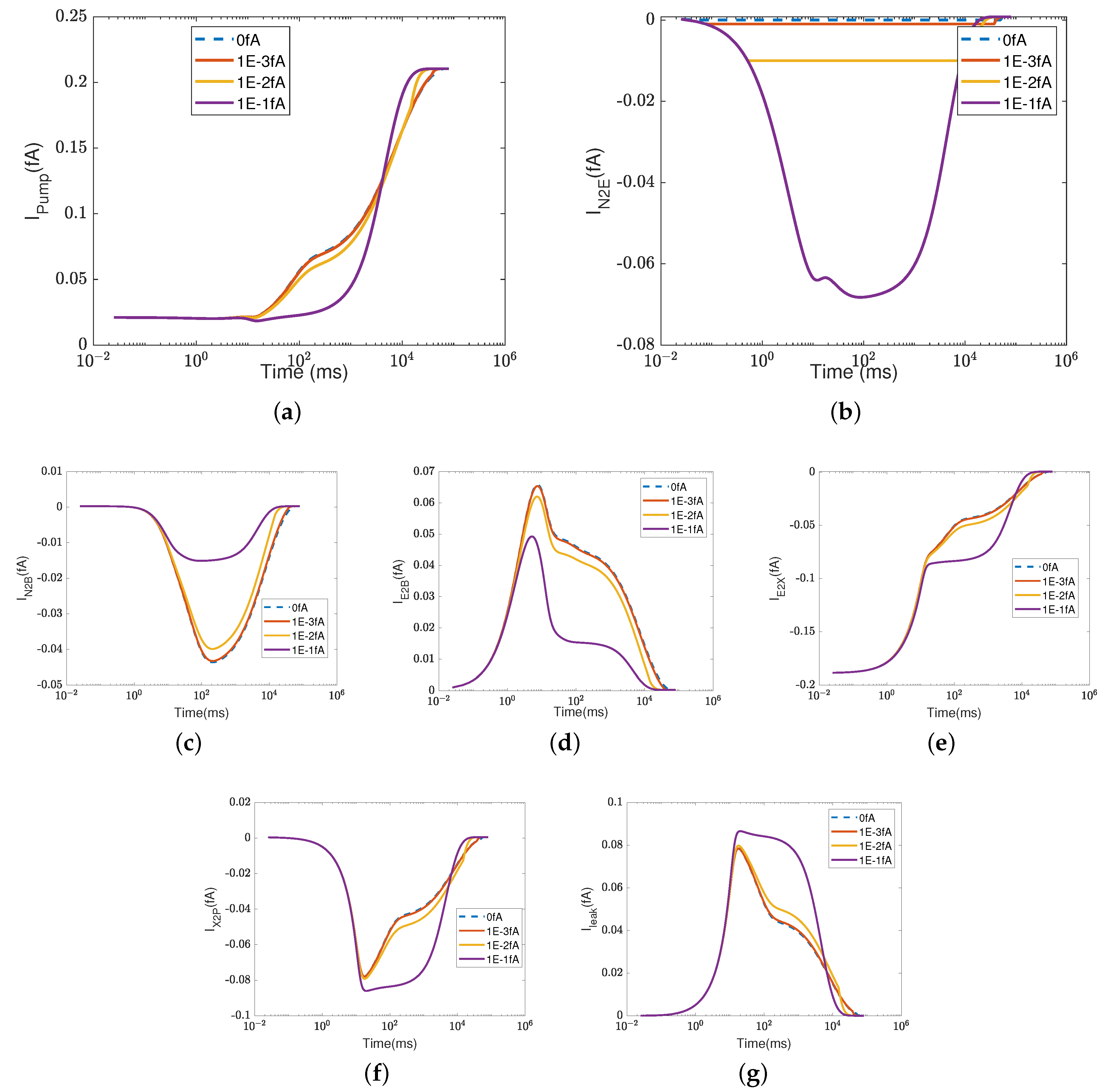
4.1. Effect of Electron Current: Input to Output Relations
Figure 2 depicts the effect of the electron current,
, on the efficiency of Complex IV. The case 1 (inside to the E rectifier) results are represented by blue circles and the case 2 (X to the outside rectifier) results are represented by red squares.
The ratios between the currents and the supplied electron current are measures of the transfer function or ’gain’ of cytochrome c oxidase. According to a previous study [
50], the ratios are
,
, and
at the normal state. These ratios mean that nominally, each input electron will bring two protons from the N side. One of the protons is used for the chemical reaction and the other one is pumped to the P side, becoming an output.
Figure 2d–h confirm that when the electron supply is sufficient (
), these ratios can be maintained. However, if the input electron current decreases (in magnitude), the reaction rate decreases linearly (see
Figure 2a) since
at equilibrium according to Equation (37d). The pump strength depends on the reaction rate (Equation (38g)), so the pump current,
, decreases hand in hand with the reaction rate.
Beyond a certain threshold, the total current between
and the PLS,
, becomes negative, provided that the rectifier is located between the inside and the E site (blue lines with circles). The protons leak back from the PLS to
. This ‘leak back’ can be seen in
Figure 2d, where the positive ratio means that
is negative (because
is negative, according to our sign conventions). In this case, protons flow back from the outside to the PLS. The accumulated protons in
increase the chemical potential,
, above
and
, which leads to more currents flowing from
to reaction site B (see
Figure 2f) and backflow from the reaction site to the N side (see
Figure 2h). The rectifier blocks direct backflow from
to the N side. The current,
, becomes zero (see
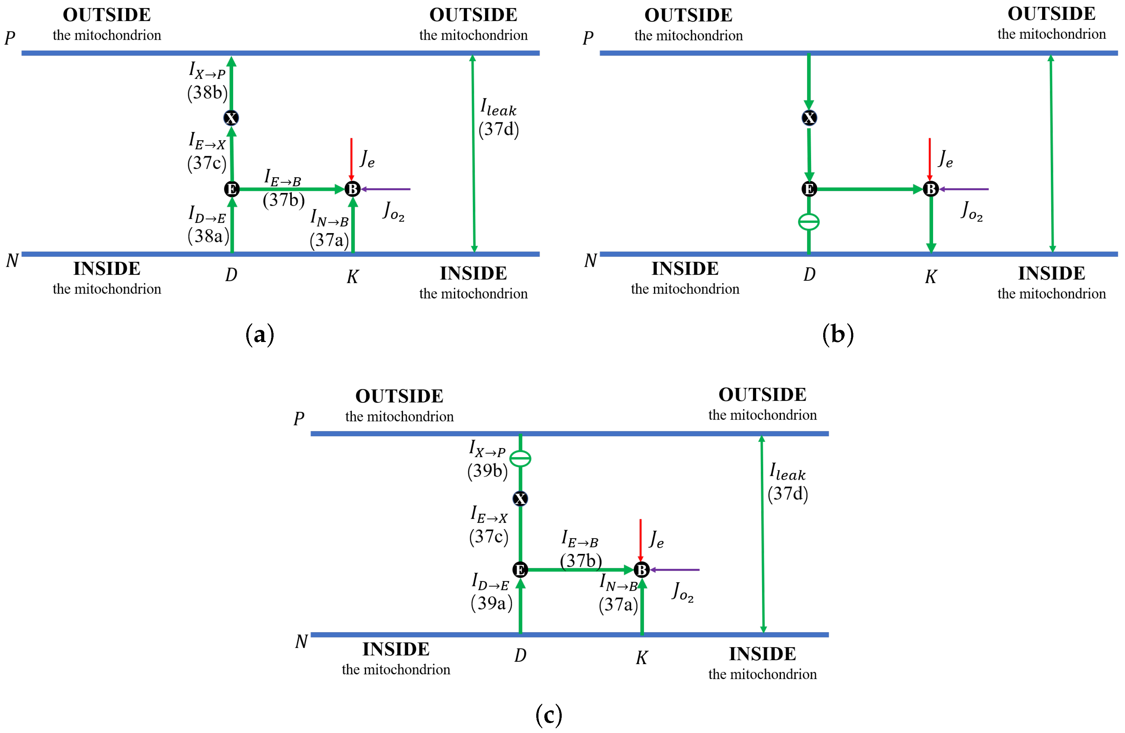
Figure 2g). The proton flow pattern in this case is shown in
Figure 3b.
The location of the rectifier is important, as the behavior differs when the rectifier is moved. When the rectifier is positioned between the PLS and the outside (red lines with squares), the backward flow from the outside to the PLS is blocked and becomes zero. Then, the current,
, also becomes zero at equilibrium according to Equation (37c), which means that
, as shown in
Figure 2b. Protons are still transported from the inside to
and then to the BNC, with
through the D channel directly to the BNC and
through the K channel.
Figure 3c shows the proton flow pattern in this case.
We suspect that the rectifier between the PLS and the outside is closer to a real biological setup because it blocks backward flow. For this reason, we mainly present the results with the rectifier between the PLS and the outside. Our approach can, of course, handle almost any location or properties of the rectifier/switch once they are specified through experiments or higher-resolution models.
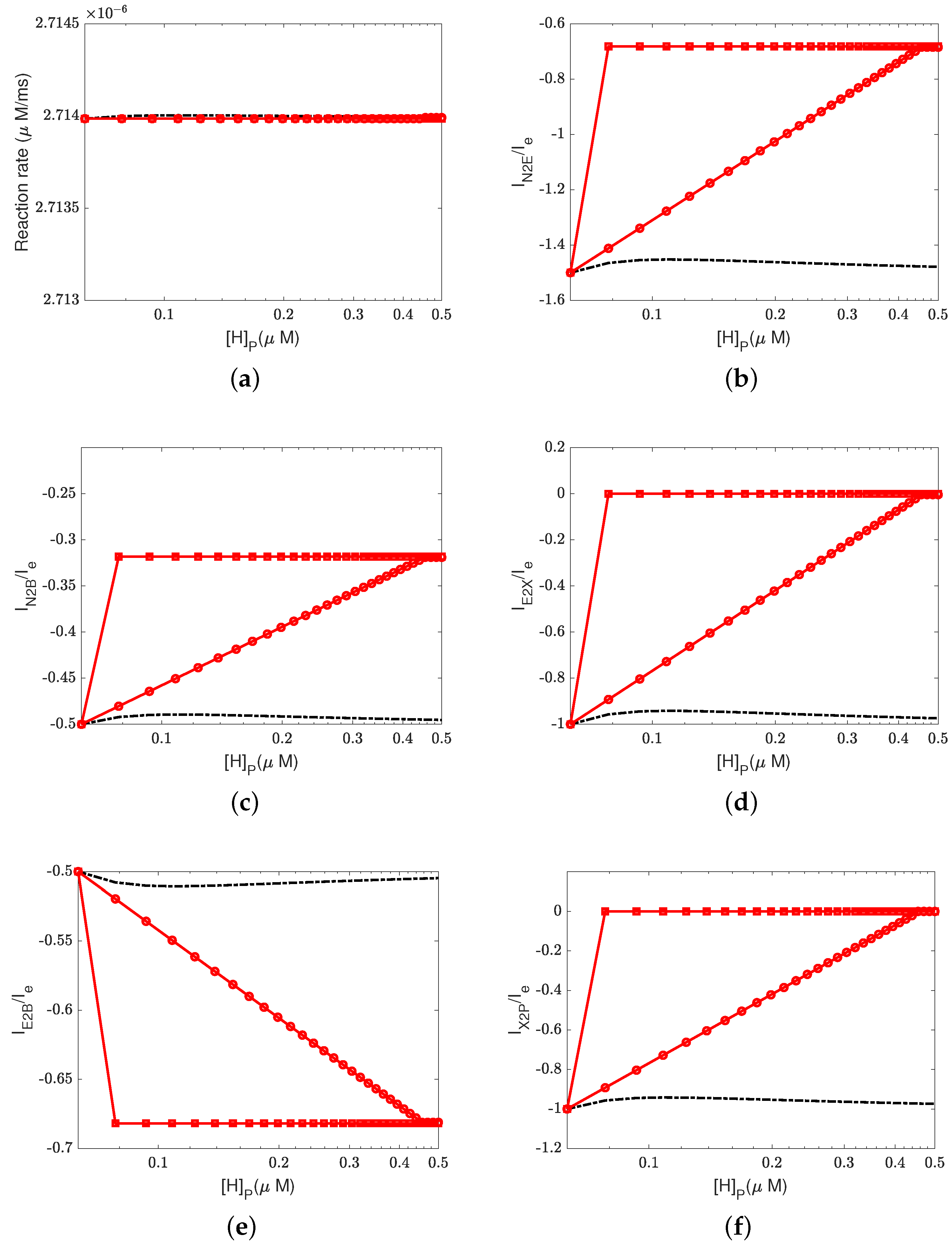
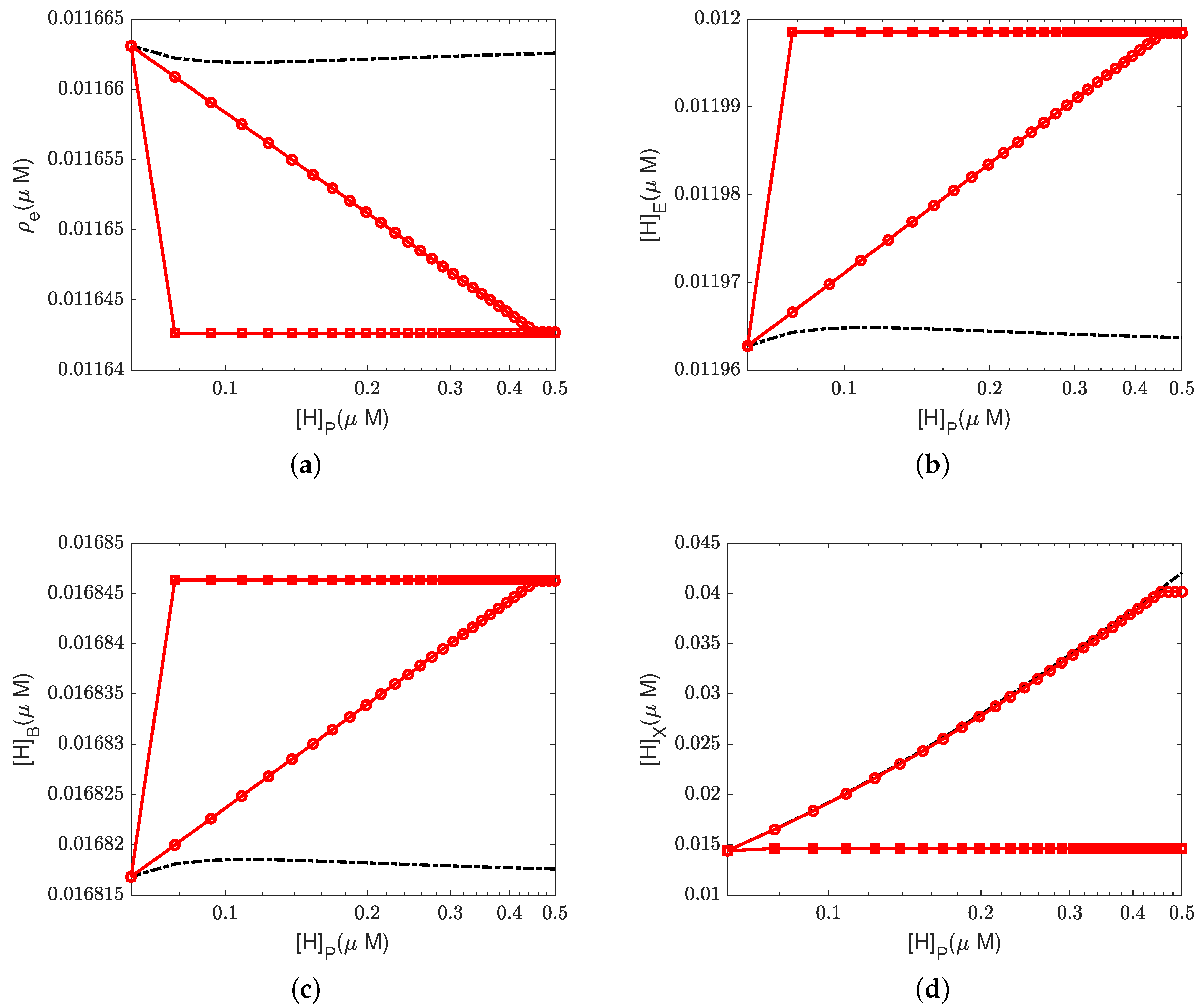
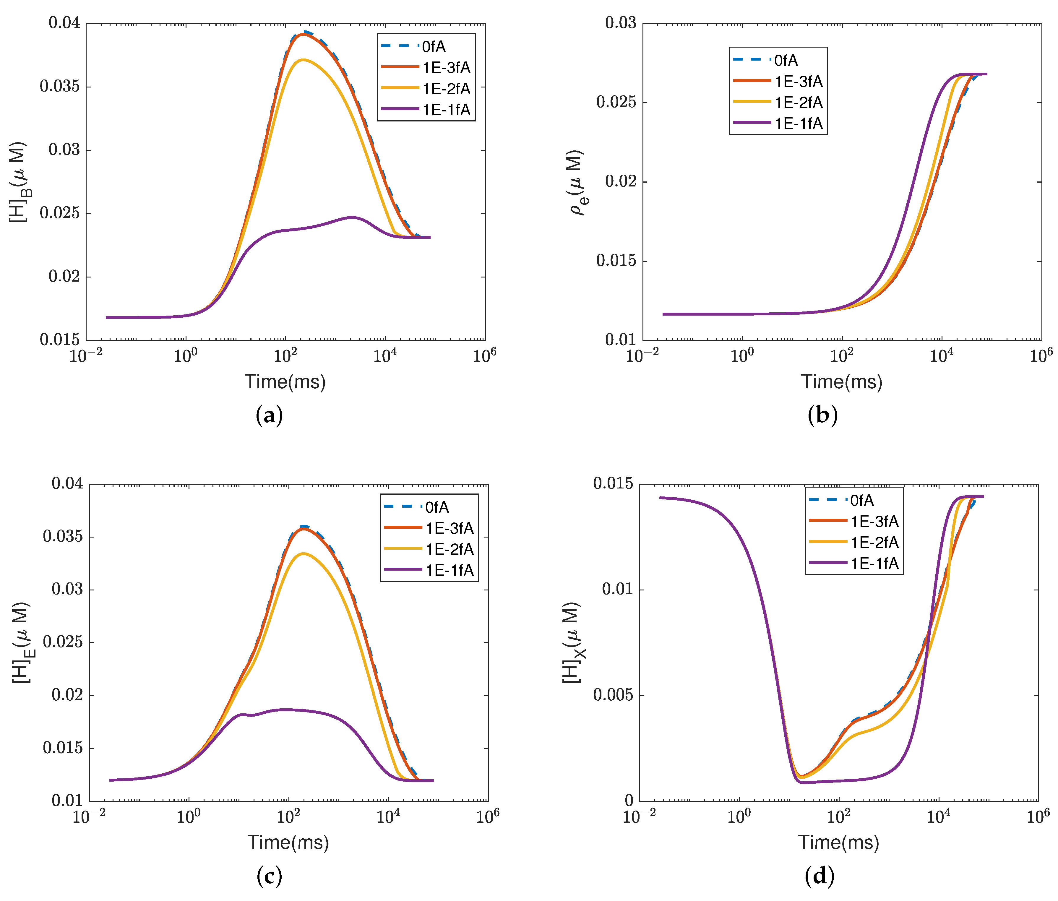
4.2. Effect of Proton Concentration
In this section, we study the effect of the proton concentrations in the inter-membrane space (outside) by increasing the default value from 0.06
M to 0.15
M.
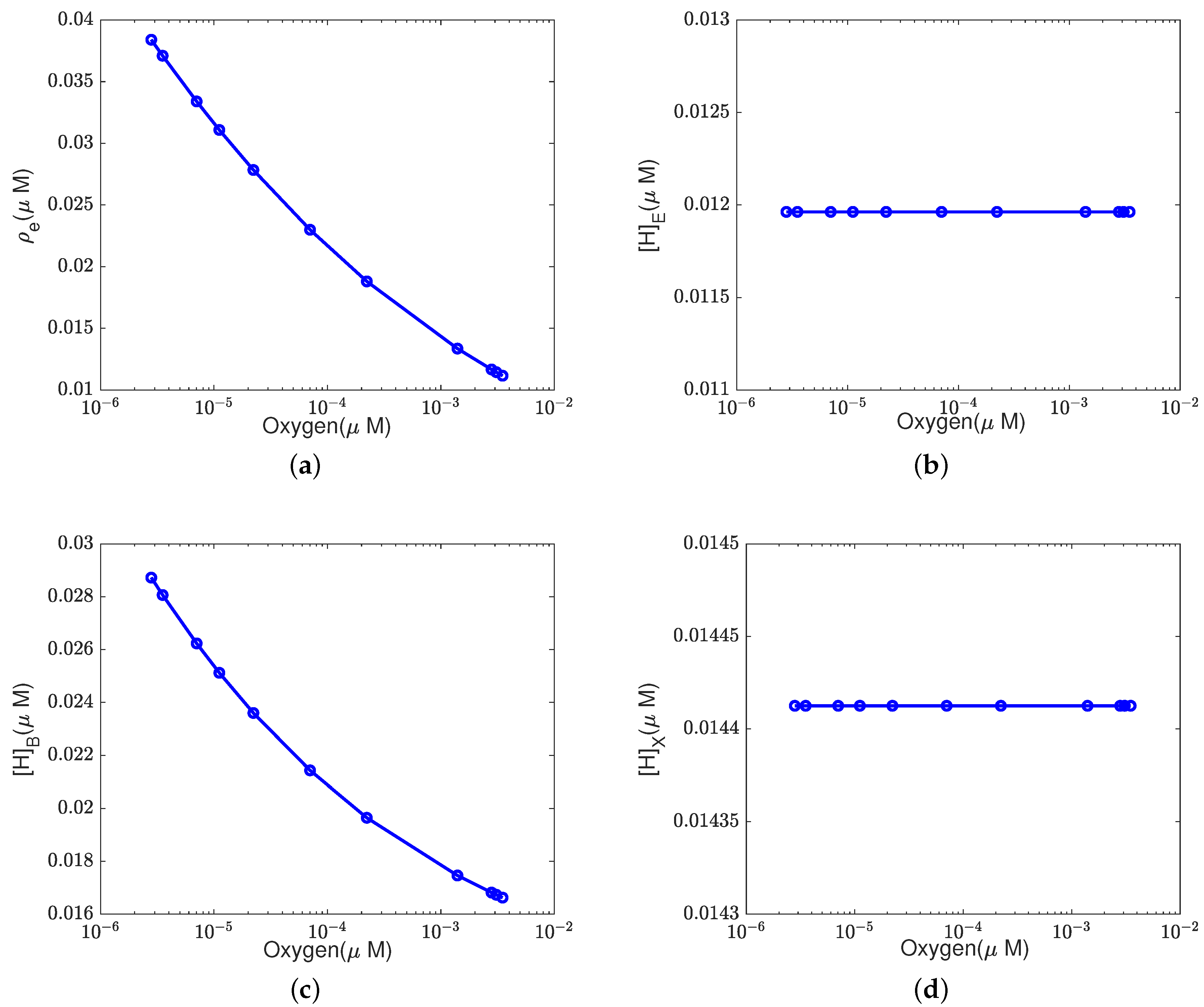
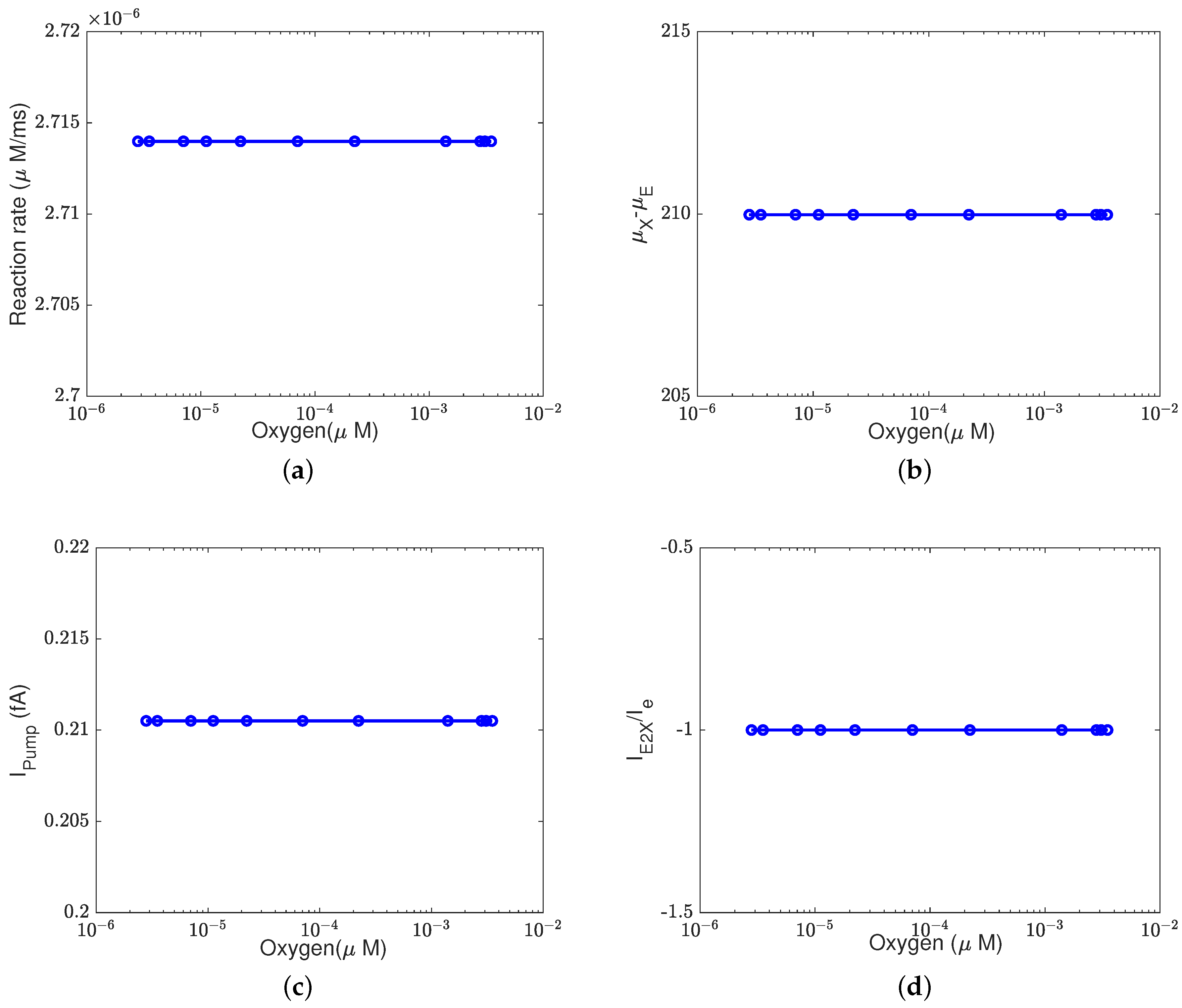
Figure 4 and
Figure 5 show the equilibrium states of the concentrations and the pump efficiency at different proton concentrations with different leak conductances
.
First,
Figure 4a illustrates that the reaction rate with different
remains constant since
at equilibrium. When the leak conductance is zero, the Complex IV efficiency does not change, i.e.,
, as shown in the flow pattern in
Figure 3a. When the shunt conductance
is higher than zero, the pump resistance increases with the outside proton concentration. This produces a decrease in the Complex IV efficiency down to zero, beyond the threshold. Then, the proton pattern is the same as in
Figure 3c, where all the protons pumped from the inside through the D and K channels are consumed by the reaction at the BNC.
The concentrations of electrons and protons at the E and B sites are small perturbations in all cases. The concentration in the PLS is almost constant with different when the leak conductance is high. However, it increases tremendously when the leak conductance is low. A high leak conductance simulates the voltage-clamp conditions, which do not describe the normal functional state of the mitochondrion. A low leak conductance presumably corresponds to the natural state in which the sum of all currents across the mitochondrion is ‘clamped’ to zero according to Kirchhoff’s current law because there is nowhere else for the current to flow.
4.3. Kirchhoff Clamp
Most of this paper describes cytochrome c oxidase embedded in a mitochondrion, approximating a preparation without other members of the respiratory chain but with otherwise normal properties. The mitochondrion is a small cell in which the interior potential is unlikely to vary substantially on a macroscopic scale; at the micron scale, the cell is much smaller than the length constant of cable theory. In such a system, Kirchhoff’s current law ensures that the sum of all currents across the mitochondrial membrane is zero. The currents are necessarily coupled by electrodynamics, regardless of whether they are coupled by chemistry. If one current increases, the sum of the others must decrease. A graph plotting one current against another will yield a definite ratio, a coupling ratio if you will, when other variables are held constant.
The various currents are coupled through the electric potential. The electrical potential contributes to the forces that drive these currents. Chemical reactions may also contribute. But even without chemical reactions, coupling can occur through the electric field. While this may seem strange in the context of classical transport biophysics, it is well established and understood in channel biophysics, which presumably follows the same laws of physics. The coupling of sodium and potassium conductances that allow the action potential to propagate is an example of coupling through the electric field without the chemical interaction of the underlying protein molecules, as we have discussed previously in this paper.
Coupling occurs because the electric field adopts the values that conserve the current, which is easy to prove using Maxwell’s equations [
96,
97]. In fact, the conservation of the current is a form of Kirchhoff’s law, so currents are clamped to one another (i.e., coupled) in a “Kirchhoff clamp” if we want to coin a phrase for what is really just the unclamped, natural situation.
If the electrical potential is controlled and is not free to adopt the values that conserve the current, a different situation occurs altogether. This situation is called a voltage clamp in electrophysiology and was invented by Cole and used by Hodgkin and Huxley to understand the mechanism of the action potential. The voltage clamp loosens the Kirchhoff clamp because it has an amplifier (that is outside the biological system) to supply the current and energy. Indeed, the Kirchhoff clamp of the natural mitochondrion is entirely removed by the currents supplied by the voltage-clamp amplifier.
In the voltage clamp, one current is not coupled to another current through the voltage. They cannot be because the voltage does not vary with the current. The result is that the coupling and flux ratios reflect the chemical coupling and not the voltage coupling in the voltage-clamp setup. The result is that nearly every experimental result is different in a voltage clamp and the natural unclamped situation.
The voltage clamp was invented to gain experimental control of currents so they can be studied, as made abundantly clear by Cole, followed by Hodgkin and Huxley, but the voltage clamp is not natural. It removes a natural form of flux coupling. Flux coupling through the electric field is absent. Flux coupling through the electric field is natural, just as natural in the mitochondrion as in the nerve, and just as natural in the generation of ATP as in the generation of the nerve signal.
It is difficult to voltage-clamp mitochondria, and preparations reconstituted into bilayers (that can be voltage-clamped) have other difficulties that experimentalists often wish to avoid. Other methods are used to simulate a voltage clamp, quite well, as it turns out.
In work on mitochondria, a voltage clamp is usually produced indirectly by artificially increasing the leak conductance. An effective carrier of potassium currents like valinomycin is often added to solutions. When valinomycin is present in large enough concentrations, it partitions into the mitochondrial membrane and the leak conductance dominates. The potential across the mitochondrial membrane is set through the equilibrium potential of the leak conductance. If valinomycin is used to increase the leak conductance, the potential is, in fact, close to the potassium equilibrium potential independent of the current because valinomycin is remarkably selective for potassium ions. Valinomycin clamps the potential to the potassium equilibrium potential.
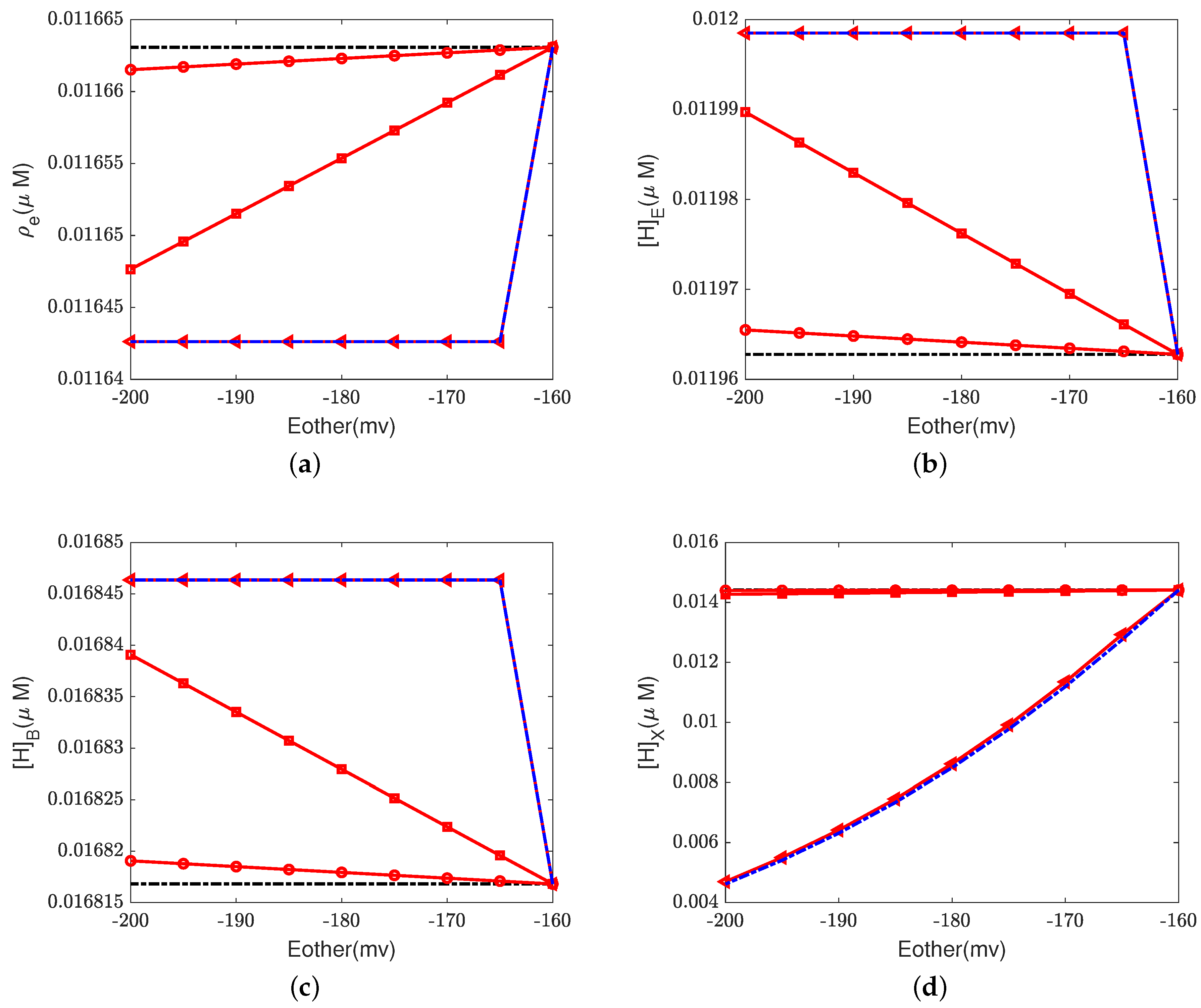
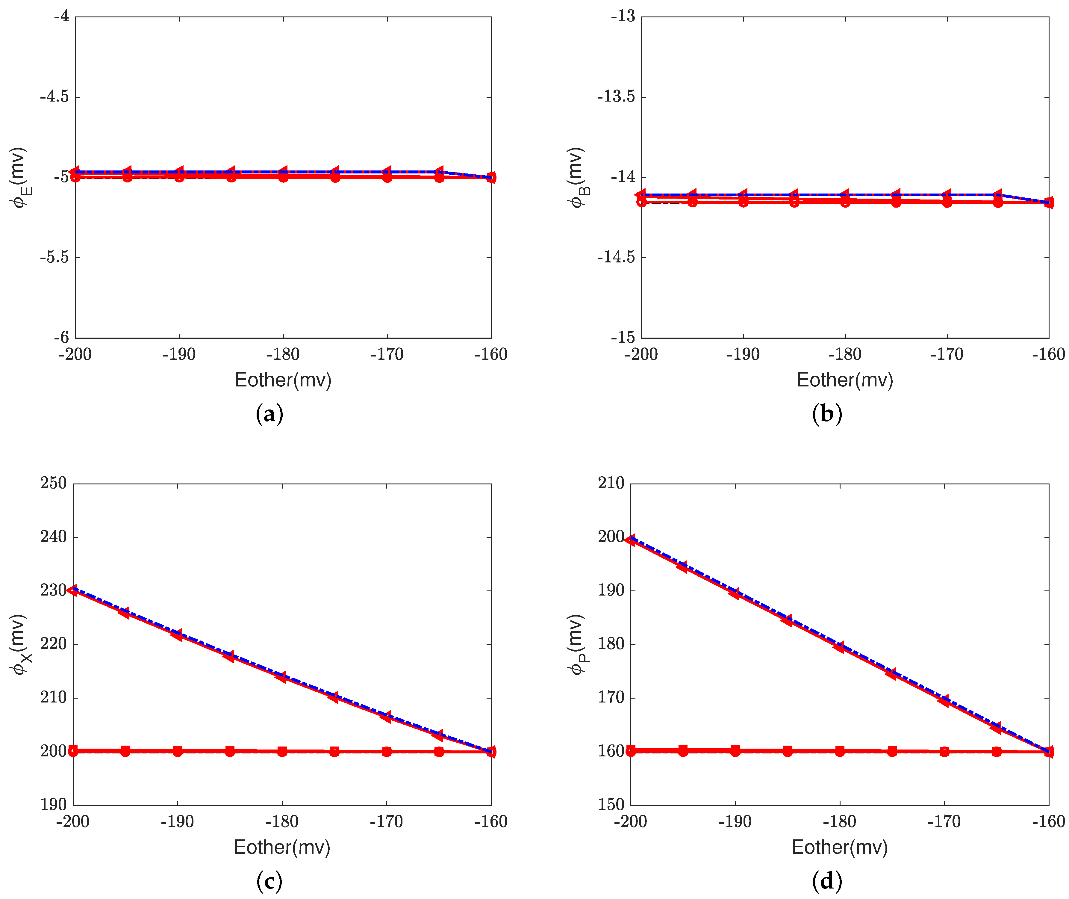
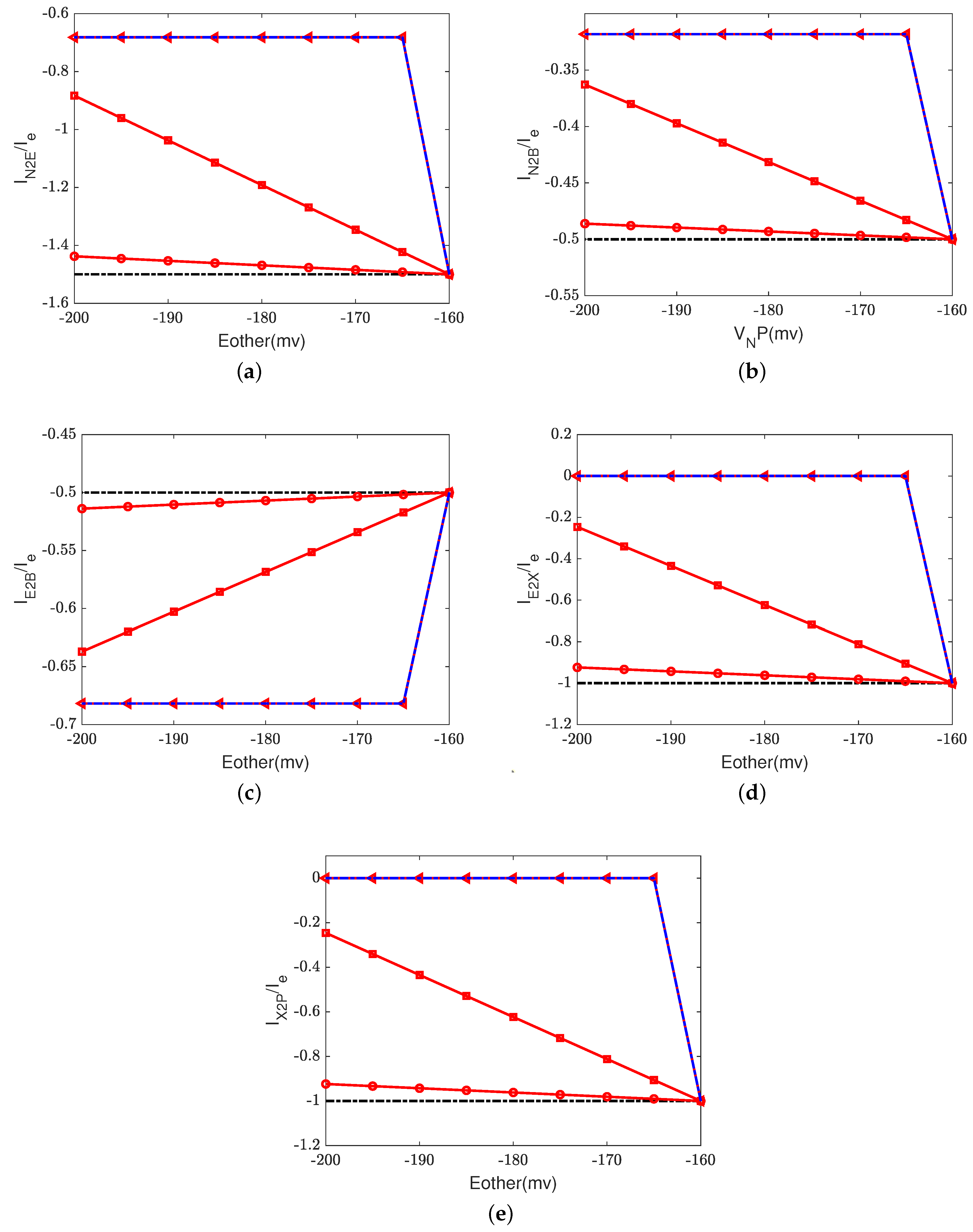
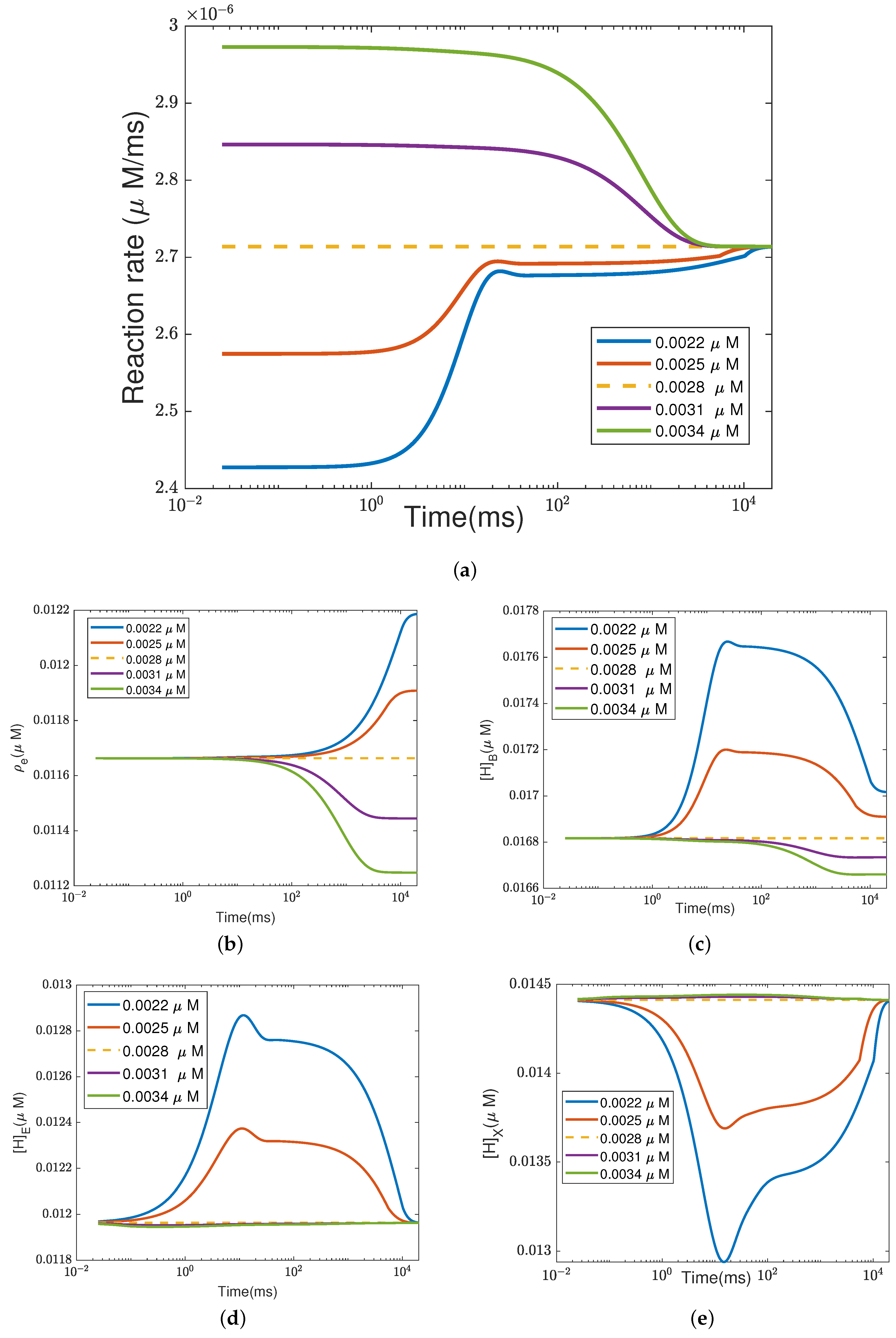
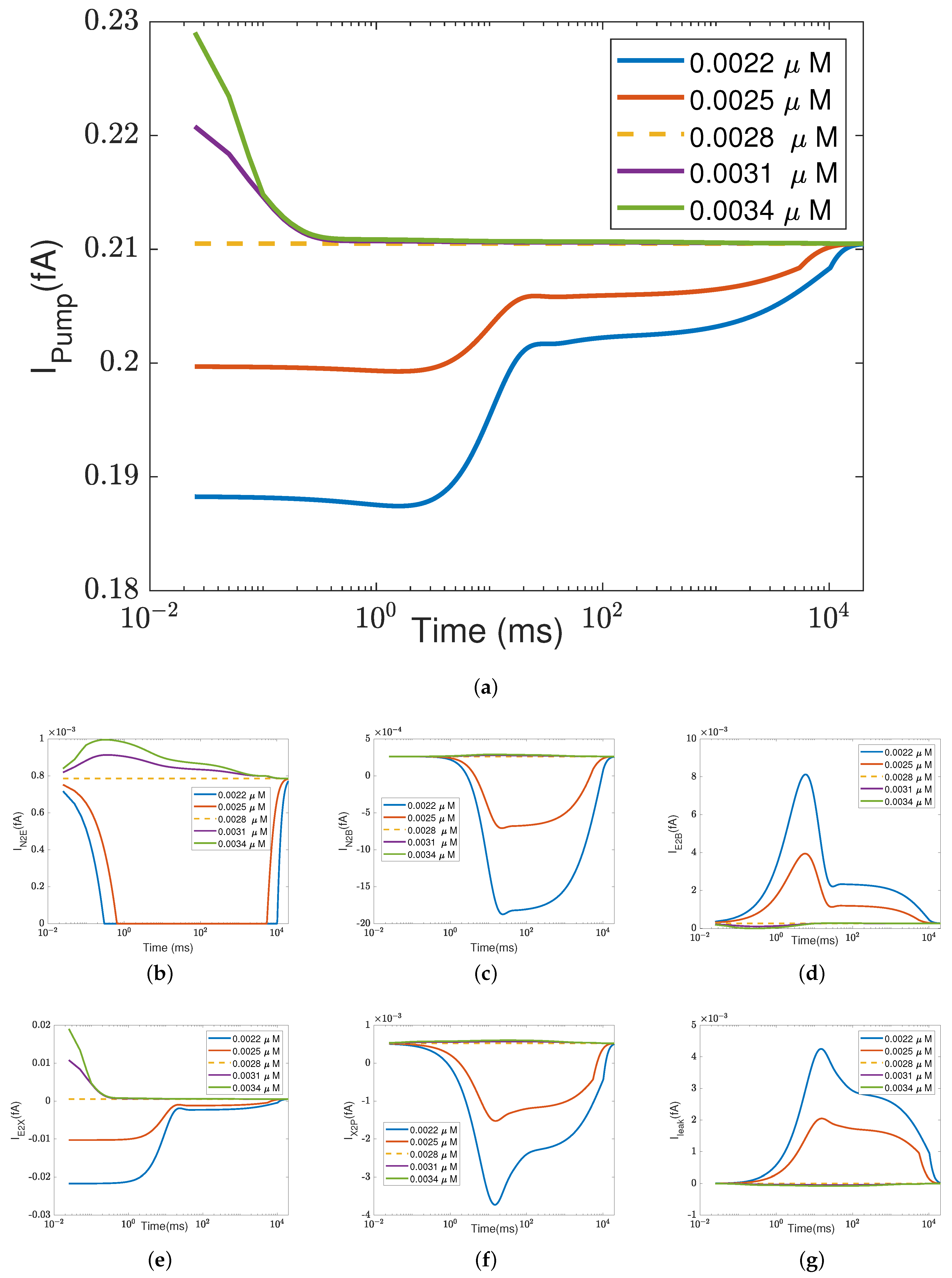
Figure 6,
Figure 7 and
Figure 8 illustrate the effect of the Nernst potential
on concentrations, electric potentials, and currents under different leak conductances.
is an approximation of the potassium equilibrium potential. The red lines with circles, squares, and triangles denote the leak conductances
and
, respectively. The black dashed lines are the results of setting zero leakage, i.e.,
, and the blue dashed lines denote the voltage-clamp results, where the electric potential at the inside,
, is set to zero and the electric potential at the outside
according to System (37).
First, we consider the natural case, where the shunt conductance
. Cytochrome c oxidase is not affected. The efficiency of Complex IV is not changed by the Nernst potential because
is always zero in this case. When
, as the Nernst potential becomes more negative, the resistance for proton pumping increases, which leads to a decrease in the proton pump efficiency. Of course, when the leak conductance is high enough, the system is nearly voltage-clamped to the equilibrium potential for the leak. The Kirchhoff clamp (red lines with triangles) is unlocked and removed through the high leak conductance. The results are the same as those of the voltage clamp (blue dashed lines).
Figure 6d,
Figure 7c,d and
Figure 8 show the differences in various quantities between voltage-clamped and unclamped natural situations.
In addition to what’s mentioned above, different parameters play different roles in proton pumping. The effects of oxygen and switch on the pump efficiency are presented in Appendices
Appendix A.1 and
Appendix A.2.
5. Discussion and Conclusions
Our study integrates Kirchhoff’s law for total currents into a comprehensive framework encompassing chemical reactions, ions, and water flows. We utilize the energy variation method rooted in complex fluid theory to deal with open systems, like the devices in our electronic technology, ion channels, and transporters. Our approach employs the electro-osmotic framework to analyze the coarse-grained dynamics of cytochrome c oxidase in the tradition of ‘master equations’, but we focus on the analysis of currents and not charges. This approach builds upon established and rigorously analyzed methods of the theory of complex fluids, extended to electrochemical open systems. These methods offer a distinctive perspective by assessing the master equations using Kirchhoff’s law for currents. Our findings demonstrate that under standard conditions, each input electron brings two protons from the mitochondrial matrix. One proton is utilized for the reaction, driving the rectification between the protein loading site (PLS) and its environment closer to biological settings.
Our work bypasses detailed specifications of individual charges, instead focusing on the flows of currents as specified by Kirchhoff’s law. Employing Maxwell’s version of Ampere’s law, we extend the circuit analysis to encompass oxidative phosphorylation and photosynthesis systems, highlighting the evolutionary incorporation of electron and ion current flows, and present a complex fluid theory-driven approach.
Our work is preliminary because it over-approximates several important biophysical mechanisms, including the water-gate switch and the oxygen reduction mechanism.
We are well aware of the need for higher resolution in later work using specific atomic-scale models that can compute the electric field, flows, and rate constants of the underlying structures, as well as atomic-scale models of the chemical reactions. Time scales of displacement (capacitive) currents have been effectively resolved in experiments despite their complexity and should be included in later versions of our model. These currents are important in understanding the switches and mechanisms through which cytochrome c oxidase couples electron flow, oxidative chemical reactions, and proton flow to make oxidative phosphorylation possible in mitochondria.
Our ‘electro-osmotic’ model is a ‘master equation’ approach that builds on the work of Hummer and Kim [
47,
48,
49] but shows how to exploit the conservation of the current in the form of Kirchhoff’s current law, without dealing with individual charges or using thermodynamic ideas best applied to systems without flows.
The current-based approach is used throughout electrical and electronic engineering to design semiconductor devices, as textbooks document (
), perhaps most eloquently, in the modern automated circuit design literature built on Kirchhoff’s law [
30]. Currents are sufficient for such automated design. Charges are not needed except in the occasional switched-capacitor networks (p. 64 of [
30]).
We extend the classical use of Kirchhoff’s law, which forms the foundation of circuit design, to include chemical reactions. We must include chemical reactions to drive currents of electrons, protons, and other ions because that is how cytochrome c oxidase functions. The essential function of cytochrome c oxidase is to convert a flow of electrons to a flow of protons from inside the mitochondrion to outside it. The electrons that are input to the cytochrome c oxidase are presented to the enzyme attached to the heme group of cytochrome c itself.
The existing literature analyzes these systems without explicitly dealing with currents, making the task either impossible (by using a theory that assumes a zero value for the fluxes being studied) or very difficult (by involving a staggering number of charges). Using currents instead of charges avoids these difficulties and has the added advantage of automatically satisfying Maxwell’s equations if the total current is used in Kirchhoff’s law.
This approach is incomplete because it does not deal with all the charges in the circuit formed by cytochrome c oxidase, but these details are not needed in the design of electronic circuits. This simple fact can be verified by examining textbooks on circuit design (as already cited).
In a circuit analysis of this type, some questions about charges need not be asked; for example, the atomic mechanism of current flow (particularly electron flow) can be ignored. The function of the circuit is independent of the details of the components of the currents in wires, for example, with only a few exceptions [
75]. Thus, we de-emphasize the atomic details of the various pathways that provide electron flow to the main reaction centers. For us, these pathways are wires. The atomic and chemical details of the electron flow in these wires are known in breathtaking detail and we are sorry that we do not seem to need to use these magnificent results, but, at this resolution, we do not.
A key biological result is that some of the coupling important for understanding the electro-osmotic properties of a mitochondrion depend on the macroscopic conservation of the current, i.e., Kirchhoff’s law applied to the entire mitochondrion. The application of Kirchhoff’s law to mitochondrial transport, and active transport in general, is not common in the literature. But Kirchhoff’s law has been used in another branch of biophysics for over eighty years. Kirchhoff’s law is the keystone of the analysis of ion channels. Kirchhoff’s law is the keystone that secures Hodgkin’s formulation of membrane biophysics, including the action potential that arches over membrane biophysics. The Hodgkin formulation provides an understanding of function, beyond less relevant molecular details, by balancing the various components of current, sodium, and potassium, summing them to zero in the appropriate (finite) geometries, like those of mitochondria, the way the keystone of an arch sums mechanical forces.
The conservation of the current provides the coupling in other biophysical applications, e.g., the generation and propagation of the action potential, linking the atomic-scale properties of ion channels of one type to the properties (e.g., opening) of another type. In a classical action potential, the opening of sodium channels is coupled to the opening of other sodium channels and the closing of potassium channels through the electric field, not by anything else. There is no steric or chemical interaction between the channels. The coupling is essential to the function of the nerve cell, but this coupling is described by a version of Maxwell’s equations (called the cable or telegrapher’s equation), not by equations of chemical kinetics. The ion channels of the action potential act independently in the chemical sense because they are so far apart, without an opportunity for short-range or chemical interactions. The ion channels are not independent, in the physiological or physical sense, however. Rather, they are coupled through the electric field. The electrical field is that which satisfies Maxwell’s equations, or their equivalent, Kirchhoff’s current law.
The historical dissociation between chemical theory and devices has obscured the significance of boundary conditions and flows. In contrast, our approach uses the principles underlying electronic circuit analysis, acknowledging the need for consistent, spatially nonuniform boundary conditions and flows in chemical systems like ion transporters and mitochondria. The application of our findings extends beyond theoretical realms, with potential applications in shaping chemical systems into functional devices, mirroring the essential properties of engineering devices.
Devices are important. Our electronic technologies are built using devices that function more or less the same way regardless of where they are located (within reasonable limits, it goes without saying, as nothing in engineering or technology is true in general, and everything exists and functions only within reasonable limits). It would obviously be useful if chemical systems could be easily and routinely shaped into devices.
Devices depend on spatially complex boundary conditions that include flows and so are open systems that usually require power supplies to function. A device has inputs and outputs with different locations and boundary equations. If the inputs and outputs are at the same location and have the same properties, there is no device! Most devices have power supplies as well as inputs and outputs. These supply flows of energy allow the device to have well-defined input–output relations that are robust and quite independent of what is connected to the input or output of the device. A transfer function relates the input to the output through a constant coefficient causal ordinary differential equation over time.
Devices maintain these properties almost entirely by using electricity and energy from power supplies. They are fundamentally nonequilibrium open systems with spatially nonuniform Dirichlet boundary conditions for the electrical potential.
Our exploration of the core Maxwell’s equations underscores the uniqueness of these field equations, offering a robust framework, even when the spatial and temporal location of charge is unknown. Polarization phenomena are understood as the response of electromechanical systems to changes in the electric field. Polarizable materials need to be analyzed as complex fluids, often with energy variation methods.
In summary, our work advances a multidisciplinary approach rooted in complex fluid theory and engineering principles, redefining the boundaries between chemical theory and engineering devices. Our methodological exploration marks a step toward a more comprehensive understanding of complex systems, bridging the gap between theoretical frameworks and technological applications in the domain of chemical systems.


