Global Dynamics of a Within-Host Model for Usutu Virus

Abstract

We propose a within-host mathematical model for the dynamics of Usutu virus infection, incorporating Crowley–Martin functional response. The basic reproduction number ${\mathfrak{R}}_0$ is found by applying the next-generation matrix approach. Depending on this threshold, parameter, global asymptotic stability of one of the two possible equilibria is also established via constructing appropriate Lyapunov functions and using LaSalle’s invariance principle. We present numerical simulations to illustrate the results and a sensitivity analysis of ${\mathfrak{R}}_0$ was also completed. Finally, we fit the model to actual data on Usutu virus titers. Our study provides new insights into the dynamics of Usutu virus infection.

1. Introduction

Viral replication and the corresponding immune response are described by within-host models. The AIDS crisis has a significant impact on the study of within-host dynamics. There are many different approaches to model, see, e.g., numerous works by Perelson [1,2,3].

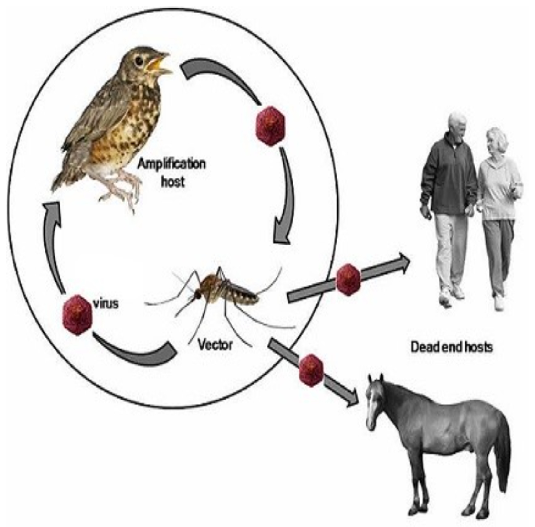
Usutu virus (abbreviated as USUV) is an emergent pathogen that is still poorly understood, despite its threat [4,5,6]. USUV, an arbovirus discovered in 1959 in the Republic of South Africa, spreads through mosquito bites, akin to West Nile fever and Zika. Its main focus is on avian neural tissues encompassing the brain and spinal cord. Beyond this, it can infiltrate blood cells, visceral organs like the spleen and liver, along with muscular tissues [7]. The name of the virus comes from the Usutu River [6]. Since its first identification, the virus has been observed in several African countries, such as Burkina Faso, Côte d’Ivoire, Morocco, Nigeria, Senegal, Uganda [8,9,10]. The virus was first detected outside Africa in 2001, killing a high number of blackbirds in Vienna [11]. Eight years later, the first European cases of human infections were reported, where it caused encephalitis in patients with weakened immune system in Italy [12]. In Africa, the most important hosts mainly are mosquitoes of the Culex genus, birds, as well as humans showing mild or severe symptoms. In Figure 1 we depict the transmission cycle of the disease, showing that the bird-mosquito-bird cycle ends in humans or horses, i.e., that the virus cannot be transmitted from one person to another. Due to its role as a potential pathogen for humans and its similarity to other emerging arboviruses, the study of this virus should be of increased interest.

Due to the mortality observed in some bird species after its introduction in Europe, the USUV has received increasing attention in many study areas [13,14,15,16,17,18], which has allowed more information to be obtained.

An excellent understanding of the dynamics of epidemic transmission can be gained by mathematical modeling. There have been numerous attempts to comprehend the Usutu virus’s dynamics of transmission and to estimate the crucial factors that affect transmission. Recently, Heitzman-Breen et al. [15] have proposed a model describing viral infection in the following form:

$$\begin{array}{cc}\hfill \frac{dT}{dt}& =-\beta TV,\hfill \\ \hfill \frac{dE}{dt}& =\beta TV-kE,\hfill \\ \hfill \frac{dI}{dt}& =kE-\delta I,\hfill \\ \hfill \frac{dV}{dt}& =pI-cV,\hfill \end{array}$$

where T denotes target cells, E stands for exposed cells, I denotes infected cells and V denotes free virus particles. The target cells get infected at rate $\beta$ and become productively infected at rate k. Productively infected cells produce virus at rate p and die at rate $\delta$. Finally, virus is cleared at rate c.

Given that many scholars have stated that the bilinear incidence function is insufficient to fully represent the infection process, our model in this study is based on a generalization of the aforementioned model utilizing a particular functional response function [19].

In the study of biomathematical models, various functional responses have been utilized, including the Holling-type I–IV, Beddington–DeAngelis and Leslie–Gower functional response. Among these, the Crowley–Martin functional response stands out for its capacity to elucidate the saturation phenomena intrinsic to viral replication, driven by the accessibility of target cells. In the realm of viral infections, a fundamental understanding exists that viral replication encounters an upper limit due to the finite availability of susceptible host cells. This nuanced dynamics, often overlooked by the traditional logistic function [20], necessitates the incorporation of nonlinear response functions in epidemiological models. The Crowley–Martin form, introduced by P. H. Crowley and E. K. Martin, emerged from their study of dragonfly populations [21]. This form is distinguished by its ability to accommodate scenarios where, counterintuitively, predation decreases despite high prey density due to increased predator density and interference among predators [22,23]. Mathematically, the Crowley–Martin functional form is expressed as $\frac{\beta TV}{(1+C_{1}T)(1+C_{2}V)}$, with $C_1,C_2$ representing nonnegative parameters denoting handling time and the degree of interference among predators, respectively, with regard to the feeding rate. This functional response finds relevance in modeling infections like the Usutu virus, where intracellular replication triggers a saturation effect on the infection rate. Moreover, its success in modeling various viral infections positions it as a logical choice for comprehending the intricate dynamics of Usutu virus infection and affords insights into strategies for disease control (see e.g., [24,25,26,27,28,29]).

The paper is structured as follows. The model is introduced in Section 2. In Section 3 we show positivity and boundedness of the solutions. The existence as well as local and global stability of equilibria are described in Section 5. Numerical simulations are given in Section 6 including interpretations in biology. The paper is closed by a short discussion.

2. Model Derivation

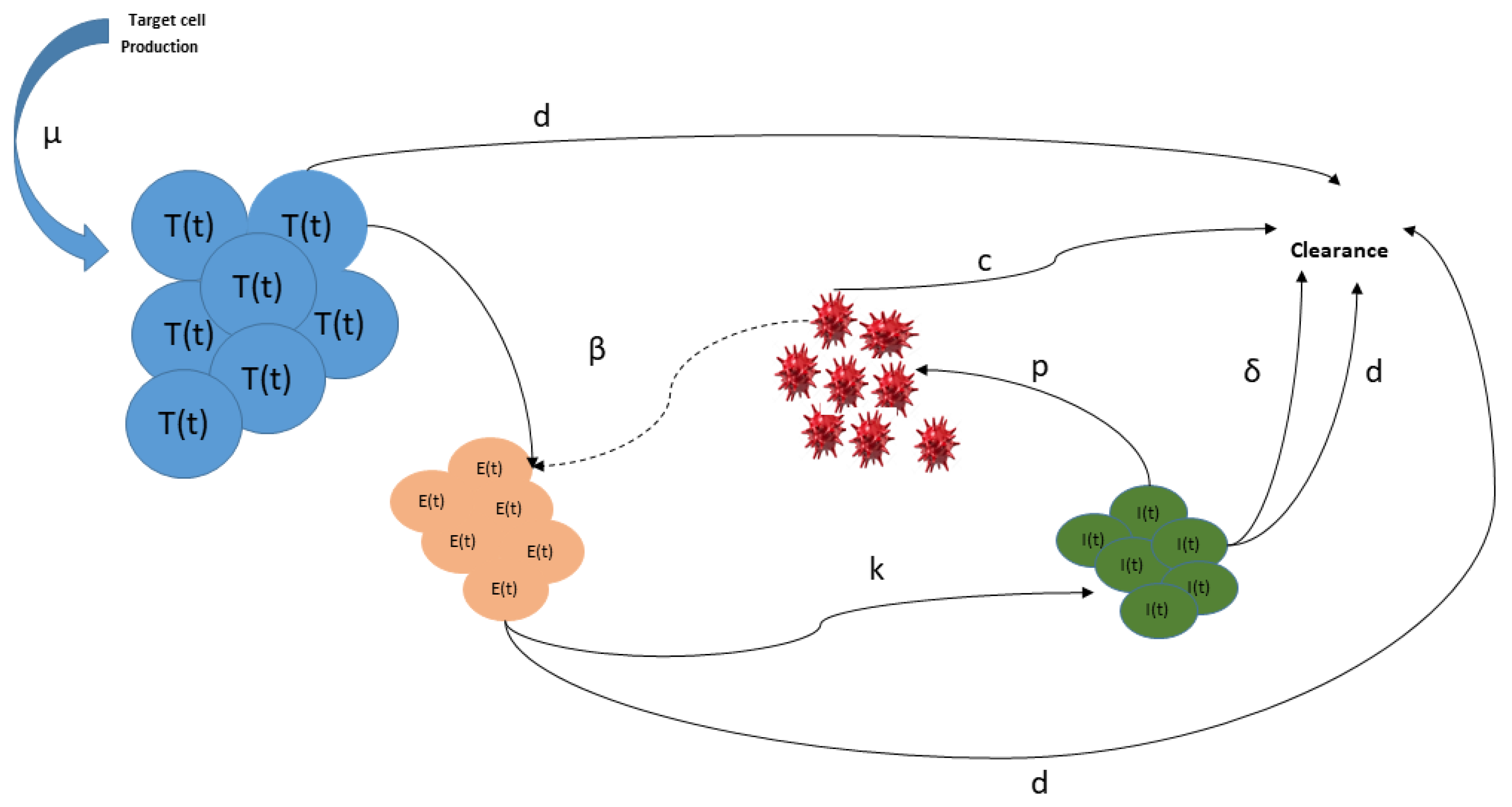
The present model represents the mechanism of transmission of the Usutu virus within the host. Based on the model suggested by Heitzman-Breen et al. [15], we divide the total cell population into healthy target cells $\left(T\right)$, exposed cells $\left(E\right)$ and infected cells $\left(I\right)$. For the number of virus particles we use the notation V. As described in the introduction, we introduce Crowley–Martin-type functional response for the infection process. Furthermore, we also include cell birth and death. The rate of the former is denoted by $\mu$, while that of the latter is denoted by d. The rest of the notations are listed in

Table 1. Parameters of model (1).

Parameter	Definition	Units
$\mu$	Birth rate	(leukocyte/mL) × ${\mathrm{days}}^{-1}$
d	Death rate	days${}^{-1}$
$\beta$	Infection rate	($\log 10$ PFU/mL)${}^{-1}$ × days${}^{-1}$
k	Transition rate from exposed to infectious	days${}^{-1}$
$\delta$	Disease-induced death rate	days${}^{-1}$
p	Production rate of virions	$\log 10$ PFU/(infected cell × day)
c	Virus clearance rate	days${}^{-1}$
$C_1$	Positive parameter describing the effects of capture rate	(leukocyte/mL)${}^{-1}$
$C_2$	Positive parameter describing the effects of capture rate	($\log 10$ PFU/mL)${}^{-1}$

and are the same as those in the introduction. The model is given as

$$\begin{array}{cc}\hfill & \frac{dT}{dt}=\mu -\frac{\beta TV}{(1+C_{1}T)(1+C_{2}V)}-dT,\hfill \\ \hfill & \frac{dE}{dt}=\frac{\beta TV}{(1+C_{1}T)(1+C_{2}V)}-kE-dE,\hfill \\ \hfill & \frac{dI}{dt}=kE-\delta I-dI,\hfill \\ \hfill & \frac{dV}{dt}=pI-cV.\hfill \end{array}$$

(1)

We note that system (1) is not specific to Usutu virus. The flow chart depicting the within-host dynamics of Usutu virus can be seen in Figure 2.

We note that here, the parameter $\beta$ has a unit different from the one in [15], which motivated our work. In fact, after a careful check of units and initial values given in [15], we came to the conclusion, that the unit $(\log 10$ PFU/mL)${}^{-1}$× days${}^{-1}$ should be used for the parameter $\beta$.

3. Positivity and Boundedness of the Solutions

Our analysis of (1) will start with studying some basic properties of the model. First we will show that any solution of (1) started from an initial condition in ${\mathbb{R}}_{+}^4$ will remain nonnegative. In fact, we have

$$\begin{array}{cc}\hfill {\left.\frac{dT}{dt}\right|}_{T=0}& =\mu >0,\hfill \\ \hfill {\left.\frac{dE}{dt}\right|}_{E=0}& =\frac{\beta TV}{(1+C_{1}T)(1+C_{2}V)}\ge 0\mathrm{for}\mathrm{all}T,E\ge 0,\hfill \\ \hfill {\left.\frac{dI}{dt}\right|}_{I=0}& =kE\ge 0\mathrm{for}\mathrm{all}E\ge 0,\hfill \\ \hfill {\left.\frac{dV}{dt}\right|}_{V=0}& =pI\ge 0.\hfill \end{array}$$

These equalities prove that ${\mathbb{R}}_{+}^4$ is positively invariant with regard to system (1).

Next, we will show that all solutions of system (1) are bounded. Considering the first equation of our system, we have

$$\frac{dT}{dt}+dT\le \mu .$$

(2)

Multiplying (2) by $e^{dt}$, we have

$$e^{dt}\frac{dT}{dt}+dT{e}^{dt}\le \mu e^{dt}.$$

After integrating both sides we get

$$T\left(t\right)\le T_0{e}^{-dt}+\frac{\mu }{d}(1-e^{-dt})\le T_0+\frac{\mu }{d},$$

which shows that T is bounded. From the second equation of (1), we have

$$\begin{array}{cc}\hfill \frac{dE}{dt}+(k+d)E& \le \frac{\beta TV}{(1+C_{1}T)(1+C_{2}V)}=\mu -dT-\frac{dT}{dt},\hfill \end{array}$$

(3)

Multiplying (3) by $e^{(k+d)t}$, we obtain

$${\left(E{e}^{(k+d)t}\right)}^{\prime }\le \mu e^{(k+d)t}-e^{kt}{\left(T{e}^{dt}\right)}^{\prime }.$$

Integrating both sides we get

$$E\left(t\right)\le E_0{e}^{-(k+d)t}+\frac{\mu }{k+d}(1-e^{-(k+d)t})-{\int }_0^t{e}^{ks}{\left(T\left(s\right)e^{ds}\right)}^{\prime }ds$$

and

$${\int }_0^t{e}^{ks}{\left(T\left(s\right)e^{ds}\right)}^{\prime }ds=T\left(t\right)e^{(k+d)t}-T_0-k{\int }_0^{t}T\left(s\right)e^{(k+d)s}ds.$$

From this, one gets

$$E\left(t\right)\le E_0+T_0+\frac{\mu }{(k+d)}+k{\int }_0^{t}T\left(s\right)e^{(k+d)(s-t)}ds.$$

As T is bounded, from this we obtain that

$$E\left(t\right)\le E_0+T_0+\frac{1}{(k+d)}\left(\mu +k\left(T_0+\frac{\mu }{d}\right)\right).$$

As a result, the boundedness of E follows.

By a similar calculation, using the above results we obtain

$$I\left(t\right)\le I_0+k(E_0+T_0+\frac{1}{k+d}\left(\mu +k\left(T_0+\frac{\mu }{d}\right)\right))$$

and

$$V\left(t\right)\le V_0+p{I}_0+pk(E_0+T_0+\frac{1}{k+d}\left(\mu +k\left(T_0+\frac{\mu }{d}\right)\right)).$$

4. Equilibria and Reproduction Number

4.1. Disease-Free Equilibrium

To find the equilibria of (1), one needs to solve the following algebraic system of equations:

$$\begin{array}{cc}\hfill 0& =\mu -\frac{\beta TV}{(1+C_{1}T)(1+C_{2}V)}-dT,\hfill \\ \hfill 0& =\frac{\beta TV}{(1+C_{1}T)(1+C_{2}V)}-kE-dE,\hfill \\ \hfill 0& =kE-\delta I-dI,\hfill \\ \hfill 0& =pI-cV.\hfill \end{array}$$

The unique disease-free equilibrium of (1) can be calculated as

$${\mathcal{E}}_0=\left(\frac{\mu }{d},0,0,0\right).$$

4.2. Basic Reproduction Number

To obtain the basic reproduction number $\left({\Re }_0\right)$, we will apply the next-generation matrix method (see e.g., [30]). For our model, the transmission matrix f and the transition matrix v take the form

$$f=\left[\begin{array}{c}\frac{\beta TV}{(1+C_{1}T)(1+C_{2}V)}\\ 0\\ 0\end{array}\right]\mathrm{and}v=\left[\begin{array}{c}-kE-dE\\ kE-\delta I-dI\\ pI-cV\end{array}\right].$$

We obtain ${\mathfrak{R}}_0$ as the spectral radius of the matrix $\left(F{V}^{-1}\right)$, where the matrices F and V are introduced as the Jacobians of f and v evaluated at the disease-free equilibrium.

These two matrices are found as

$$\begin{array}{cc}\hfill F& =\left(\begin{array}{ccc}0& 0& \beta \frac{\mu }{d+C_1\mu }\\ 0& 0& 0\\ 0& 0& 0\end{array}\right)\mathrm{and}\hfill \\ \hfill V& =\left(\begin{array}{ccc}-d-k& 0& 0\\ k& -d-\delta & 0\\ 0& p& -c\end{array}\right).\hfill \end{array}$$

for our model Hence, the next generation matrix has the form

$$F{V}^{-1}=\left(\begin{array}{ccc}-\frac{\beta k\mu p}{c(d+C_1\mu )(d+\delta )(d+k)}& -\frac{\beta \mu p}{c(d+C_1\mu )(d+\delta )}& -\frac{\beta \mu }{c(d+C_1\mu )}\\ 0& 0& 0\\ 0& 0& 0\end{array}\right),$$

from which the basic reproduction number ${\mathfrak{R}}_0$ can be calculated as

$${\mathfrak{R}}_0=\frac{p\beta k\mu }{c(d+\delta )(d+k)(d+C_1\mu )}.$$

4.3. Infection Equilibrium

Lemma 1. 

Model (1) has a unique positive equilibrium ${\mathcal{E}}_1=\left(T^{*},E^{*},I^{*},V^{*}\right)$, if ${\mathfrak{R}}_0>1$.

Proof. 

To find infection equilibria of (1), one has to solve the system of algebraic equations

$$\begin{array}{cc}\hfill \mu -d{T}^{*}-\frac{\beta T^{*}{V}^{*}}{(1+C_1{T}^{*})(1+C_2{V}^{*})}& =0,\hfill \\ \hfill \frac{\beta T^{*}{V}^{*}}{(1+C_1{T}^{*})(1+C_2{V}^{*})}-k{E}^{*}-d{E}^{*}& =0,\hfill \\ \hfill k{E}^{*}-\delta I^{*}-d{I}^{*}& =0,\hfill \\ \hfill p{I}^{*}-c{V}^{*}& =0.\hfill \end{array}$$

Solving this system, we obtain the second order equation

$$C_{1}bdkp{T}^{\ast 2}+\left[pk\left(\beta +b(d-C_1\mu )\right)-C_{1}c(d+k)(d+\delta )\right]T^{*}-\left(C_{2}k\mu p+c(d+k)(d+\delta )\right)=0$$

for $T^{*}$. This equation admits two solutions given by

$$\begin{array}{cc}\hfill T_{+}^{*}=& \frac{C_{1}c(d+\delta )(d+k)-pk(\beta +b(d-C_1\mu ))}{2C_1{C}_{2}dkp}\hfill \\ & +\frac{\sqrt{{(pk(\beta +C_2(d-C_1\mu ))-C_{1}c(d+\delta )(d+k))}^2+4C_1{C}_{2}dpk(C_{2}k\mu p+c(d+\delta )(d+k)}}{2C_1{C}_{2}dkp},\hfill \\ \hfill T_{-}^{*}=& \frac{C_{1}c(d+\delta )(d+k)-pk(\beta +C_2(d-C_1\mu ))}{2C_1{C}_{2}dkp}\hfill \\ & -\frac{\sqrt{{(pk(\beta +C_2(d-C_1\mu ))-C_{1}c(d+\delta )(d+k))}^2+4C_1{C}_{2}dpk(C_{2}k\mu p+c(d+\delta )(d+k)}}{2C_1{C}_{2}dkp}.\hfill \end{array}$$

Furthermore, $T_{+}^{*}\times T_{-}^{*}=\frac{-\left(C_{2}k\mu p+c(d+k)(d+\delta )\right)}{C_1{C}_{2}dkp}<0$, meaning that $T_{+}^{*}$ and $T_{-}^{*}$ have different signs. Considering that

$$\begin{array}{c}\sqrt{{(pk(\beta +C_2(d-C_1\mu ))-C_{1}c(d+\delta )(d+k))}^2+4C_1{C}_{2}dpk(C_{2}k\mu p+c(d+\delta )(d+k)}\hfill \\ \hfill >C_{1}c(d+\delta )(d+k)-pk(\beta +C_2(d-C_1\mu )),\end{array}$$

we obtain that $T_{-}^{*}<0$ and $T_{+}^{*}>0$.

The coordinates $E^{*},I^{*}$ and $V^{*}$ of the infection equilibrium can be obtained as

$$E^{*}=\frac{1}{k+d}\left(\mu -d{T}^{*}\right),I^{*}=\frac{k}{d+\delta }{E}^{*}\mathrm{and}{V}^{*}=\frac{p}{c}{I}^{*}.$$

It remains to show that all of these are positive for ${\mathfrak{R}}_0>1$. Clearly, we only need to show this for $E^{*}$. We show that the relation ${\mathfrak{R}}_0>1$ implies $\mu -d{T}^{*}>0$. Indeed,

$$\begin{array}{cc}\hfill \mu -d{T}^{*}=& \frac{-C_{1}c(d+\delta )(d+k)+pk(\beta +C_2(d+C_1\mu ))}{2C_1{C}_{2}kp}\hfill \\ & -\frac{\sqrt{{(pk(\beta +C_2(d-C_1\mu ))-C_{1}c(d+\delta )(d+k))}^2+4C_1{C}_{2}dpk(C_{2}k\mu p+c(d+\delta )(d+k)}}{2C_1{C}_{2}kp}.\hfill \end{array}$$

Taking the squares of both terms in the enumerator, we obtain

$$\begin{array}{cc}\hfill & {\left(-C_{1}c(d+\delta )(d+k)+pk(\beta +C_2(d+C_1\mu ))\right)}^2\hfill \\ \hfill & -{\left(pk(\beta +C_2(d-C_1\mu ))-C_{1}c(d+\delta )(d+k)\right)}^2\hfill \\ \hfill & +4C_1{C}_{2}dpk(C_{2}k\mu p+c(d+\delta )(d+k))\hfill \\ \hfill =& \frac{4C_1{C}_{2}pk}{c(d+\delta )(d+k)(d+C_1\mu )}\left({\mathfrak{R}}_0-1\right).\hfill \end{array}$$

From this, one can see that ${\mathfrak{R}}_0>1$ implies

$$\begin{array}{c}-C_{1}c(d+\delta )(d+k)+pk(\beta +C_2(d+C_1\mu ))\hfill \\ \hfill >\sqrt{{(pk(\beta +C_2(d-C_1\mu ))-C_{1}c(d+\delta )(d+k))}^2+4C_1{C}_{2}dpk(C_{2}k\mu p+c(d+\delta )(d+k)}.\end{array}$$

Therefore, $\mu -d{T}^{*}>0$. From this, we obtain that (1) has a unique positive equilibrium

$${\mathcal{E}}_1=\left(T^{*},E^{*},I^{*},V^{*}\right),if{\mathfrak{R}}_0>1.$$

□

5. Stability Analysis

5.1. Local Stability of the Disease-Free Equilibrium

One easily obtains the below result concerning the local asymptotic stability of the trivial equilibrium.

Theorem 1. 

If ${\mathfrak{R}}_0<1$, then ${\mathcal{E}}_0$ is locally asymptotically stable.

Proof. 

To prove the statement, we substitute ${\mathcal{E}}_0$ into the Jacobian of (1) to obtain

$$J_{{\mathcal{E}}_0}=\left(\begin{array}{cccc}-d& 0& 0& -\beta \frac{\mu }{d+C_1\mu }\\ 0& -(d+k)& 0& \beta \frac{\mu }{d+C_1\mu }\\ 0& k& -(d+\delta )& 0\\ 0& 0& p& -c\end{array}\right).$$

The characteristic equation of (1) evaluated at the disease-free equilibrium is

$$(d+\lambda )\left((c+\lambda )(d^2+d\delta +dk+\delta k+2d\lambda +\delta \lambda +k\lambda +{\lambda }^2)-\frac{p\beta k\mu }{d+C_1\mu }\right).$$

After development we get

$$\begin{array}{cc}\hfill & c{d}^3+c{d}^{2}k+c{d}^2\delta +cdk\delta -\frac{d\left(p\beta k\mu \right)}{d+C_1\mu }\hfill \\ \hfill & +\left(3cd+3d^2+ck+2dk+c\delta +2d\delta +k\delta \right){\lambda }^2+(c+3d+k+\delta ){\lambda }^3+{\lambda }^4\hfill \\ & +\lambda \left(3c{d}^2+d^3+2cdk+d^{2}k+2cd\delta +d^2\delta +ck\delta +dk\delta -\frac{p\beta k\mu }{d+C_1\mu }\right).\hfill \end{array}$$

To simplify, let us introduce the notations

$$\begin{array}{cc}\hfill l_1& =\left(3cd+3d^2+ck+2dk+c\delta +2d\delta +k\delta \right),\hfill \\ \hfill l_2& =c{d}^3+c{d}^{2}k+c{d}^2\delta +cdk\delta -\frac{d\left(p\beta k\mu \right)}{d+C_1\mu }=cd(d+\delta )(d+k)(1-{\mathfrak{R}}_0),\hfill \\ \hfill l_3& =(c+3d+k+\delta ),\hfill \\ \hfill l_4& =\left(3c{d}^2+d^3+2cdk+d^{2}k+2cd\delta +d^2\delta +ck\delta +dk\delta -\frac{p\beta k\mu }{d+C_1\mu }\right)\hfill \\ & =c(d+\delta )(d+k)\left(d\left(\frac{1}{c}+\frac{1}{d+\delta }+\frac{1}{d+k}\right)+(1-{\mathfrak{R}}_0)\right).\hfill \end{array}$$

Applying the Routh–Hurwitz stability criterion from [31] and following [32,33], the conditions for all roots to have negative real parts are

$$l_3{l}_1-l_4>0,\frac{(l_3{l}_1-l_4)l_4-l_3^2{l}_2}{l_3{l}_1-l_4}>0\mathrm{and}{l}_2>0$$

After calculation we obtain

$$\begin{array}{cc}\hfill l_3{l}_1-l_4=& \frac{\beta k\mu p}{C_1\mu +d}+c^2(3d+\delta +k)+c{(3d+\delta +k)}^2+8d^3+8d^2(\delta +k)\hfill \\ \hfill & +2d\left({\delta }^2+k^2+3\delta k\right)+\delta k(\delta +k),\hfill \\ \hfill l_2=& cd(d+\delta )(d+k)(1-{\mathfrak{R}}_0),\hfill \\ \hfill \frac{(l_3{l}_1-l_4)l_4-l_3^2{l}_2}{l_3{l}_1-l_4}=& c(d+\delta )(d+k)\left(d(\frac{1}{c}+\frac{1}{d+\delta }+\frac{1}{d+k})+(1-{\mathfrak{R}}_0)\right).\hfill \end{array}$$

If ${\mathfrak{R}}_0<1$, then $l_1,l_2,l_3,l_4,l_3{l}_1-l_4,l_3{l}_2,\mathrm{and}\frac{(l_3{l}_1-l_4)l_4-l_3^2{l}_2}{l_3{l}_1-l_4}$ are positive. Therefore, applying the Routh–Hurwitz criterion, ${\mathcal{E}}_0$ is locally asymptotically stable.  □

5.2. Global Stability

This subsection is devoted to the study of the global asymptotic stability of the two equilibria of model (1) depending on the basic reproduction number by constructing appropriate Lyapunov functions [34,35,36,37,38,39,40].

Let us denote by f the function

$$f\left(x\right)=x-lnx-1.$$

It is clear that $f\left(x\right)\ge 0$ for any $x>0$, furthermore, $f\left(1\right)=0$ holds.

To simplify the calculation, we introduce the notation $\eta =(d+k)(d+\delta )$.

5.2.1. Global Stability of the Disease-Free Equilibrium

Theorem 2. 

If ${\mathfrak{R}}_0<1$, then the disease-free equilibrium ${\mathcal{E}}_0$ is globally asymptotically stable.

Proof. 

Let us define the global Lyapunov function $L_0$ as

$$L_0(T,E,I,V)=\frac{d}{\eta (d+C_1\mu )}\left(T-\frac{\mu }{d}-\frac{\mu }{d}\log \left(\frac{Td}{\mu }\right)\right)+\frac{E}{\eta }+\frac{1}{k(d+\delta )}I+\frac{1}{pk}V$$

One easily obtains that $L_0(T,E,I,V)\ge 0$, while $L_0(T,E,I,V)=0$ holds if and only if $T=T_0$ and $E=I=V=0$. Let us now determine the derivative of $L_0$ along solutions of system (1). We obtain

$$\begin{array}{cc}\hfill \frac{d{L}_0}{dt}{|}_{\left(1\right)}=& \frac{d}{\eta (d+C_1\mu )}\dot{T}-\frac{1}{\eta (d+C_1\mu )}\frac{\mu }{T}\dot{T}+\frac{\dot{E}}{\eta }+\frac{1}{k(d+\delta )}\dot{I}+\frac{1}{pk}\dot{V}\hfill \\ \hfill =& \frac{d}{\eta (d+C_1\mu )}\left(\mu -\frac{\beta TV}{(1+C_{1}T)(1+C_{2}V)}-dT\right)-\frac{1}{\eta (d+C_1\mu )}\frac{\mu }{T}\left(\mu -\frac{\beta TV}{(1+C_{1}T)(1+C_{2}V)}-dT\right)\hfill \\ & +\frac{\frac{\beta TV}{(1+C_{1}T)(1+C_{2}V)}-(k+d)E}{\eta }+\frac{1}{k(d+\delta )}\left(kE-\delta I-dI\right)+\frac{1}{pk}\left(pI-cV\right)\hfill \\ \hfill =& \frac{d}{\eta (d+C_1\mu )}\left[2\mu -dT-\frac{{\mu }^2}{dT}\right]-\frac{1}{k}I-\frac{d}{\eta (d+a\mu )}\frac{\beta TV}{(1+C_{1}T)(1+C_{2}V)}+\frac{\mu }{\eta (d+C_1\mu )}\frac{\beta V}{(1+C_{1}T)(1+C_{2}V)}\hfill \\ & +\frac{\beta TV}{\eta (1+C_{1}T)(1+C_{2}V)}+\frac{1}{k}I-\frac{c}{pk}V\hfill \\ \hfill =& -\frac{1}{T\eta (d+C_1\mu )}{\left(dT-\mu \right)}^2+\frac{c}{pk}\frac{V}{(1+C_{2}V)}\hfill \\ & \left[\frac{pk}{c}\left(-\frac{d}{\eta (d+C_1\mu )}\frac{\beta T}{1+C_{1}T}+\frac{\mu }{\eta (d+C_1\mu )}\frac{\beta }{1+C_{1}T}+\frac{\beta T}{\eta (1+C_{1}T)}\right)-(1+C_{2}V)\right]\hfill \\ \hfill =& -\left[\frac{1}{T\eta (d+C_1\mu )}{\left(dT-\mu \right)}^2+\frac{bc}{pk(1+C_{2}V)}{V}^2\right]+\frac{c}{pk}\frac{V}{(1+C_{2}V)}\left({\mathfrak{R}}_0-1\right).\hfill \end{array}$$

From the above calculation we conclude that $\frac{d{L}_0}{dt}{|}_{\left(1\right)}\le 0$, if ${\mathfrak{R}}_0<1$. It is evident that $\frac{d{L}_0}{dt}{|}_{\left(1\right)}=0$ if and only if $T=T_0$ and $E=I=V=0$. Thus, the maximum compact invariant set in $\{(T,E,I,V)/\frac{d{L}_0}{dt}{|}_{\left(1\right)}=0\}$ consists of the only point ${\mathcal{E}}_0=\left(T_0,0,0,0\right)$. Therefore, it follows from LaSalle’s invariance principle that the non-infection steady state ${\mathcal{E}}_0$ is globally asymptotically stable if ${\mathfrak{R}}_0<1$.  □

5.2.2. Global Stability of the Infection Equilibrium Point

Theorem 3. 

If ${\mathfrak{R}}_0>1$, then the infection equilibrium ${\mathcal{E}}_1$ is globally asymptotically stable.

Proof. 

Let us define the Lyapunov function

$$\begin{array}{cc}\hfill L_1(T,E,I,V)=& \frac{1}{\eta }\left(T-T^{*}-{\int }_{T^{*}}^T\frac{(d+k)E^{*}(1+C_1\tau )(1+C_2{V}^{*})}{\beta \tau V^{*}}d\tau \right)\hfill \\ & +\frac{1}{\eta }\left(E-E^{*}-E^{*}ln\frac{E}{E^{*}}\right)+\frac{1}{k(d+\delta )}\left(I-I^{*}-I^{*}ln\frac{I}{I^{*}}\right)\hfill \\ & +\frac{1}{pk}\left(1+C_2{V}^{*}\right)\left(V-V^{*}-{\int }_{V^{*}}^V\frac{(d+k)E^{*}(1+C_1{T}^{*})(1+C_2\tau )}{\beta \tau T^{*}}d\tau \right)\hfill \end{array}$$

We have $L_1(T,E,I,V)\ge 0$, while $L_1(T,E,I,V)=0$ is equivalent to $T=T^{*}, E=E^{*}, I=I^{*}, V=V^{*}$. The derivative of the Lyapunov function $L_1(T,E,I,V)$ with respect to (1) can be calculated as

$$\begin{array}{cc}\hfill \frac{d{L}_1}{dt}{|}_{\left(1\right)}=& \frac{1}{\eta }\dot{T}-\frac{1}{\eta }\frac{(d+k)E^{*}(1+C_{1}T)(1+C_2{V}^{*})}{\beta T{V}^{*}}\dot{T}+\frac{1}{\eta }\dot{E}-\frac{E^{*}}{\eta }\frac{\dot{E}}{E}+\frac{1}{k(d+\delta )}\dot{I}-\frac{I^{*}}{k(d+k)}\frac{\dot{I}}{I}\hfill \\ & +\frac{1}{pk}\left(1+C_2{V}^{*}\right)\left(\dot{V}-\frac{(d+k)E^{*}(1+C_1{T}^{*})(1+C_{2}V)}{\beta T^{*}V}\dot{V}\right)\hfill \\ \hfill =& \frac{1}{\eta }\dot{T}+\frac{1}{\eta }\dot{E}+\frac{1}{k(d+\delta )}\dot{I}+\frac{1}{pk}\dot{V}-\frac{E^{*}(1+C_{1}T)(1+C_2{V}^{*})}{(d+\delta )\beta T{V}^{*}}\dot{T}-\frac{E^{*}}{\eta }\frac{\dot{E}}{E}-\frac{I^{*}}{k(d+k)}\frac{\dot{I}}{I}+\frac{1}{pk}{C}_2{V}^{*}\dot{V}\hfill \\ & -\frac{1}{pk}\left(1+C_2{V}^{*}\right)\frac{(d+k)E^{*}(1+C_1{T}^{*})(1+C_{2}V)}{\beta T^{*}V}\dot{V}\hfill \end{array}$$

Since $\left(T^{*},E^{*},I^{*},V^{*}\right)$ is a positive equilibrium point of (1), we have

$$\frac{\beta T^{*}{V}^{*}}{(1+C_1{T}^{*})(1+C_2{V}^{*})}-(d+k)E^{*}=0.$$

This means that

$$-\frac{1}{pk}\frac{V^{*}}{V}\dot{V}=\frac{1}{pk}{C}_2{V}^{*}\dot{V}-\frac{1}{pk}(1+C_2{V}^{*})\frac{(d+k)E^{*}(1+C_1{T}^{*})(1+C_{2}V)}{\beta V{T}^{*}}\dot{V}.$$

Using this, we obtain

$$\begin{array}{cc}\hfill \frac{d{L}_1}{dt}{|}_{\left(1\right)}=& \frac{1}{\eta }\dot{T}+\frac{1}{\eta }\dot{E}+\frac{1}{k(d+\delta )}\dot{I}+\frac{1}{pk}\dot{V}-\frac{E^{*}(1+C_{1}T)(1+C_2{V}^{*})}{(d+\delta )\beta T{V}^{*}}\dot{T}-\frac{E^{*}}{\eta }\frac{\dot{E}}{E}-\frac{I^{*}}{k(d+k)}\frac{\dot{I}}{I}-\frac{1}{pk}\frac{V^{*}}{V}\dot{V}\hfill \\ \hfill =& \frac{\mu }{\eta }-\frac{dT}{\eta }-\frac{c}{pk}V-\frac{E^{*}(1+C_{1}T)(1+C_2{V}^{*})}{(d+\delta )\beta T{V}^{*}}\left(\mu -\frac{\beta TV}{(1+C_{1}T)(1+C_{2}V)}-dT\right)\hfill \\ & -\frac{1}{\eta }\frac{E^{*}}{E}\left(\frac{\beta TV}{(1+C_{1}T)(1+C_{2}V)}-(d+k)E\right)-\frac{1}{k(d+\delta )}\frac{I^{*}}{I}\left(kE-(d+\delta )I\right)-\frac{1}{pk}\frac{V^{*}}{V}\left(pI-cV\right).\hfill \end{array}$$

From the positive equilibrium of (1), we have

$$\begin{array}{cc}\hfill \mu & =d{T}^{*}+(d+k)E^{*},\hfill \\ \hfill (d+k)E^{*}& =\frac{\beta T^{*}{V}^{*}}{(1+C_1{T}^{*})(1+C_2{V}^{*})},\hfill \\ \hfill V^{*}& =\frac{kp}{c}\frac{E^{*}}{(d+\delta )},\hfill \\ \hfill I^{*}& =\frac{k{E}^{*}}{(d+\delta )}.\hfill \end{array}$$

Substituting the expressions obtained for the coordinates of the infection equilibrium, we get

$$\begin{array}{c}\frac{E^{*}(1+C_{1}T)(1+C_2{V}^{*})}{(d+\delta )\beta T{V}^{*}}\left(\mu -\frac{\beta TV}{(1+C_{1}T)(1+C_{2}V)}-dT\right)\hfill \\ =\frac{T^{*}}{T}\frac{1+C_{1}T}{1+C_1{T}^{*}}\frac{d{T}^{*}}{\eta }+\frac{T^{*}}{T}\frac{1+C_{1}T}{1+C_1{T}^{*}}\frac{E^{*}}{(d+\delta )}-\frac{1+C_{1}T}{1+C_1{T}^{*}}\frac{d{T}^{*}}{\eta }-\frac{V}{V^{*}}\frac{1+C_2{V}^{*}}{1+C_{2}V}\frac{E^{*}}{(d+\delta )},\hfill \end{array}$$

$$\frac{1}{\eta }\frac{E^{*}}{E}\left(\frac{\beta TV}{(1+C_{1}T)(1+C_{2}V)}-(d+k)E\right)=\frac{E^{*}}{(d+\delta )}\left(\frac{T{E}^{*}V}{T^{*}E{V}^{*}}\frac{(1+C_1{T}^{*})(1+C_2{V}^{*})}{(1+C_{1}T)(1+C_{2}V)}-1\right),$$

$$\frac{1}{k(d+\delta )}\frac{I^{*}}{I}\left(kE-(d+\delta )I\right)=\frac{E^{*}}{(d+\delta )}\left(\frac{I^{*}E}{I{E}^{*}}-1\right),$$

$$\frac{1}{pk}\frac{V^{*}}{V}\left(pI-cV\right)=\frac{E^{*}}{(d+\delta )}\left(\frac{V^{*}I}{V{I}^{*}}-1\right).$$

Then,

$$\begin{array}{cc}\hfill \frac{d{L}_1}{dt}{|}_{\left(1\right)}=& \frac{d{T}^{*}}{\eta }+\frac{E^{*}}{(d+\delta )}-\frac{dT}{\eta }-\frac{E^{*}}{(d+\delta )}\frac{V}{V^{*}}-\frac{T^{*}}{T}\frac{1+C_{1}T}{1+C_1{T}^{*}}\frac{d{T}^{*}}{\eta }-\frac{T^{*}}{T}\frac{1+C_{1}T}{1+C_1{T}^{*}}\frac{E^{*}}{(d+\delta )}+\frac{1+C_{1}T}{1+C_1{T}^{*}}\frac{d{T}^{*}}{\eta }\hfill \\ & +\frac{V}{V^{*}}\frac{1+C_2{V}^{*}}{1+C_{2}V}\frac{E^{*}}{(d+\delta )}-\frac{E^{*}}{(d+\delta )}\left(\frac{T{E}^{*}V}{T^{*}E{V}^{*}}\frac{(1+C_1{T}^{*})(1+C_2{V}^{*})}{(1+C_{1}T)(1+C_{2}V)}-1\right)-\frac{E^{*}}{(d+\delta )}\left(\frac{I^{*}E}{I{E}^{*}}-1\right)\hfill \\ & -\frac{E^{*}}{(d+\delta )}\left(\frac{V^{*}I}{V{I}^{*}}-1\right)\hfill \\ \hfill =& \frac{d{T}^{*}}{\eta }\left(1-\frac{T}{T^{*}}-\frac{T^{*}}{T}\frac{1+C_{1}T}{1+C_1{T}^{*}}+\frac{1+C_{1}T}{1+C_1{T}^{*}}\right)+\frac{E^{*}}{(d+\delta )}\left(1-\frac{V}{V^{*}}+\frac{V}{V^{*}}\frac{1+C_2{V}^{*}}{1+C_{2}V}\right)\hfill \\ & +\frac{E^{*}}{(d+\delta )}\left(3-\frac{T^{*}}{T}\frac{1+C_{1}T}{1+C_1{T}^{*}}-\frac{T{E}^{*}V}{T^{*}E{V}^{*}}\frac{(1+C_1{T}^{*})(1+C_2{V}^{*})}{(1+C_{1}T)(1+C_{2}V)}-\frac{V^{*}I}{V{I}^{*}}-\frac{I^{*}E}{I{E}^{*}}\right)\hfill \\ \hfill =& -\frac{d}{\eta T(1+C_1{T}^{*})}{\left(T-T^{*}\right)}^2+\frac{E^{*}}{(d+\delta )}\left(-1-\frac{V}{V^{*}}+\frac{V}{V^{*}}\frac{1+C_2{V}^{*}}{1+C_{2}V}+\frac{1+C_{2}V}{1+C_2{V}^{*}}\right)\hfill \\ & +\frac{E^{*}}{(d+\delta )}\left(5-\frac{T^{*}}{T}\frac{1+C_{1}T}{1+C_1{T}^{*}}-\frac{T{E}^{*}V}{T^{*}E{V}^{*}}\frac{(1+C_1{T}^{*})(1+C_2{V}^{*})}{(1+C_{1}T)(1+C_{2}V)}-\frac{V^{*}I}{V{I}^{*}}-\frac{I^{*}E}{I{E}^{*}}-\frac{1+C_{2}V}{1+C_2{V}^{*}}\right)\hfill \\ \hfill =& -\frac{d}{\eta T(1+C_1{T}^{*})}{\left(T-T^{*}\right)}^2-\frac{b{E}^{*}}{(d+\delta )V^{*}(1+C_{2}V)(1+C_2{V}^{*})}{\left(V-V^{*}\right)}^2\hfill \\ & +\frac{E^{*}}{(d+\delta )}\left(5-\frac{T^{*}}{T}\frac{1+C_{1}T}{1+C_1{T}^{*}}-\frac{T{E}^{*}V}{T^{*}E{V}^{*}}\frac{(1+C_1{T}^{*})(1+C_2{V}^{*})}{(1+C_{1}T)(1+C_{2}V)}-\frac{V^{*}I}{V{I}^{*}}-\frac{I^{*}E}{I{E}^{*}}-\frac{1+C_{2}V}{1+C_2{V}^{*}}\right).\hfill \end{array}$$

Since

$$\log \frac{T^{*}(1+C_{1}T)}{T(1+C_1{T}^{*})}+\log \frac{T{E}^{*}V(1+C_1{T}^{*})(1+C_2{V}^{*})}{T^{*}(1+C_{1}T)(1+C_{2}V)}+\log \frac{V^{*}I}{V{I}^{*}}+\log \frac{I^{*}E}{I{E}^{*}}+\log \frac{1+C_{2}V}{1+C_2{V}^{*}}=0,$$

we have

$$\begin{array}{cc}\hfill 5-& \frac{T^{*}}{T}\frac{1+C_{1}T}{1+C_1{T}^{*}}-\frac{T{E}^{*}V}{T^{*}E{V}^{*}}\frac{(1+C_1{T}^{*})(1+C_2{V}^{*})}{(1+C_{1}T)(1+C_{2}V)}-\frac{V^{*}I}{V{I}^{*}}-\frac{I^{*}E}{I{E}^{*}}-\frac{1+C_{2}V}{1+C_2{V}^{*}}\hfill \\ \hfill =& \left(1-\frac{T^{*}}{T}\frac{1+C_{1}T}{1+C_1{T}^{*}}+\log \frac{T^{*}(1+C_{1}T)}{T(1+C_1{T}^{*})}\right)+(1-\frac{T{E}^{*}V}{T^{*}E{V}^{*}}\frac{(1+C_1{T}^{*})(1+C_2{V}^{*})}{(1+C_{1}T)(1+C_{2}V)}\hfill \\ & +\log \frac{T{E}^{*}V(1+C_1{T}^{*})(1+C_2{V}^{*})}{T^{*}(1+C_{1}T)(1+C_{2}V)})+\left(1-\frac{V^{*}I}{V{I}^{*}}+\log \frac{V^{*}I}{V{I}^{*}}\right)\hfill \\ & +\left(1-\frac{I^{*}E}{I{E}^{*}}+\log \frac{I^{*}E}{I{E}^{*}}\right)+\left(1-\frac{1+C_{2}V}{1+C_2{V}^{*}}+\log \frac{1+C_{2}V}{1+C_2{V}^{*}}\right)\le 0.\hfill \end{array}$$

From the above calculation we conclude that $\frac{d{L}_1}{dt}{|}_{\left(1\right)}\le 0$. It is evident that $\frac{d{L}_1}{dt}{|}_{\left(1\right)}=0$ if and only if $(T=T^{*},E=E^{*},I=I^{*},$ and $V=V^{*})$. Hence, the maximum compact invariant set in $\{(T,E,I,V)\mid \frac{d{L}_1}{dt}{|}_{\left(1\right)}=0\}$ is the singleton set ${\mathcal{E}}_1=\left(T^{*},E^{*},I^{*},V^{*}\right)$. Therefore, according to LaSalle’s invariance principle, the infection equilibrium point ${\mathcal{E}}_1$ is globally asymptotically stable.  □

6. Numerical Simulation

For the purpose of supporting the analytic results derived above we present some numerical results for system (1).

Table 2. Parameters of the model and their values in Figure 3.

Parameter	Value for Figure 3a	Value for Figure 3b
$\mu$	1.37	1
d	0.6	0.304
$\beta$	0.234	0.056
k	0.35	0.385
$\delta$	1	0.22
p	788	6344
c	15.65	15
$C_1$	0.284	0.013
$C_2$	0.039	0.007
$T\left(0\right)$	0.081	6344
$E\left(0\right)$	0.171	0.005
$I\left(0\right)$	0.156	0.004
$V\left(0\right)$	0.274	0.107

summarizes the parameters used.

6.1. Examples for Two Scenarios Corresponding to Theorems 2 and 3

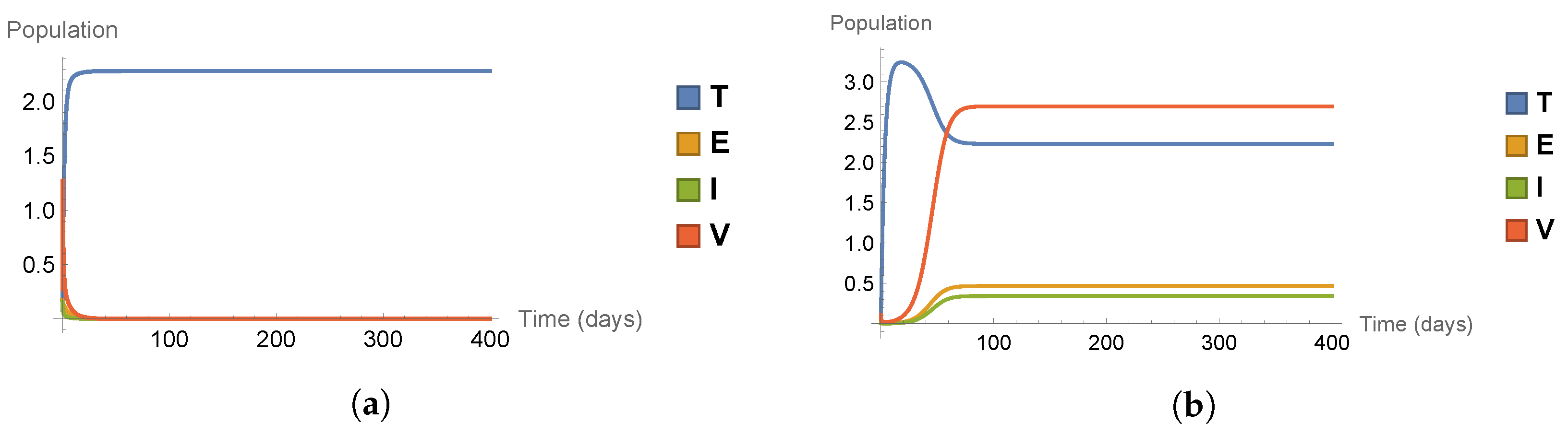
In this subsection, we present numerical simulations to support and illustrate the theoretical results. We will study two scenarios, corresponding to the two cases of disease extinction in case of ${\mathfrak{R}}_0<1$ and disease persistence in case of ${\mathfrak{R}}_0>1$. The solution curves of system (1) in both cases are shown in Figure 3.

In the first scenario (a), corresponding to ${\mathfrak{R}}_0<1$, we have a disease-free equilibrium point (disease fails to establish), the target cell population levels off at a positive equilibrium level, but the exposed, the infected, and the virus cells fail to establish and tend to 0. In the second scenario (b), corresponding to ${\mathfrak{R}}_0>1$, we have a stable infection equilibrium point, all four cell types settle in an equilibrium value.

6.2. Sensitivity Analysis of the Basic Reproduction Number

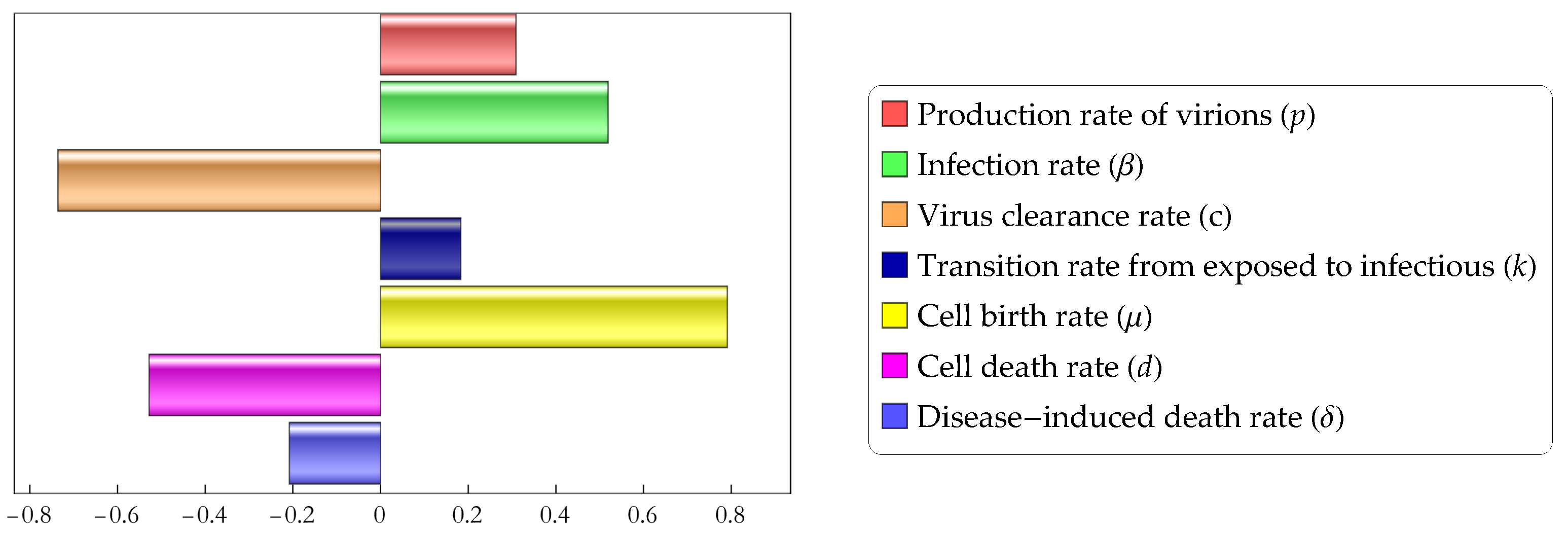
In this subsection, we perform a sensitivity analysis to study how different parameters affect the magnitude of the basic reproduction number ${\mathfrak{R}}_0$. In order to do so, we perform Partial Rank Correlation Coefficients (PRCC) analysis. This method enables us to assess the effect of each input parameter on the outcome parameter (${\mathfrak{R}}_0$ in our case). Parameters with a positive PRCC value are positively correlated with the outcome parameter, i.e., increasing any of the will increase the basic reproduction number, while those with a negative PRCC value are negatively correlated with ${\mathfrak{R}}_{\mathfrak{0}}$ meaning that an increase of their value will result in a decrease of the basic reproduction number. The results of the analysis, shown in Figure 4, suggest that cell birth rate has the largest positive effect on the basic reproduction number, followed by the infection rate $\beta$ and the production rate of virions p, while virus clearance rate c and cell death rate d are the parameters which most efficiently decrease the value of ${\mathfrak{R}}_0$.

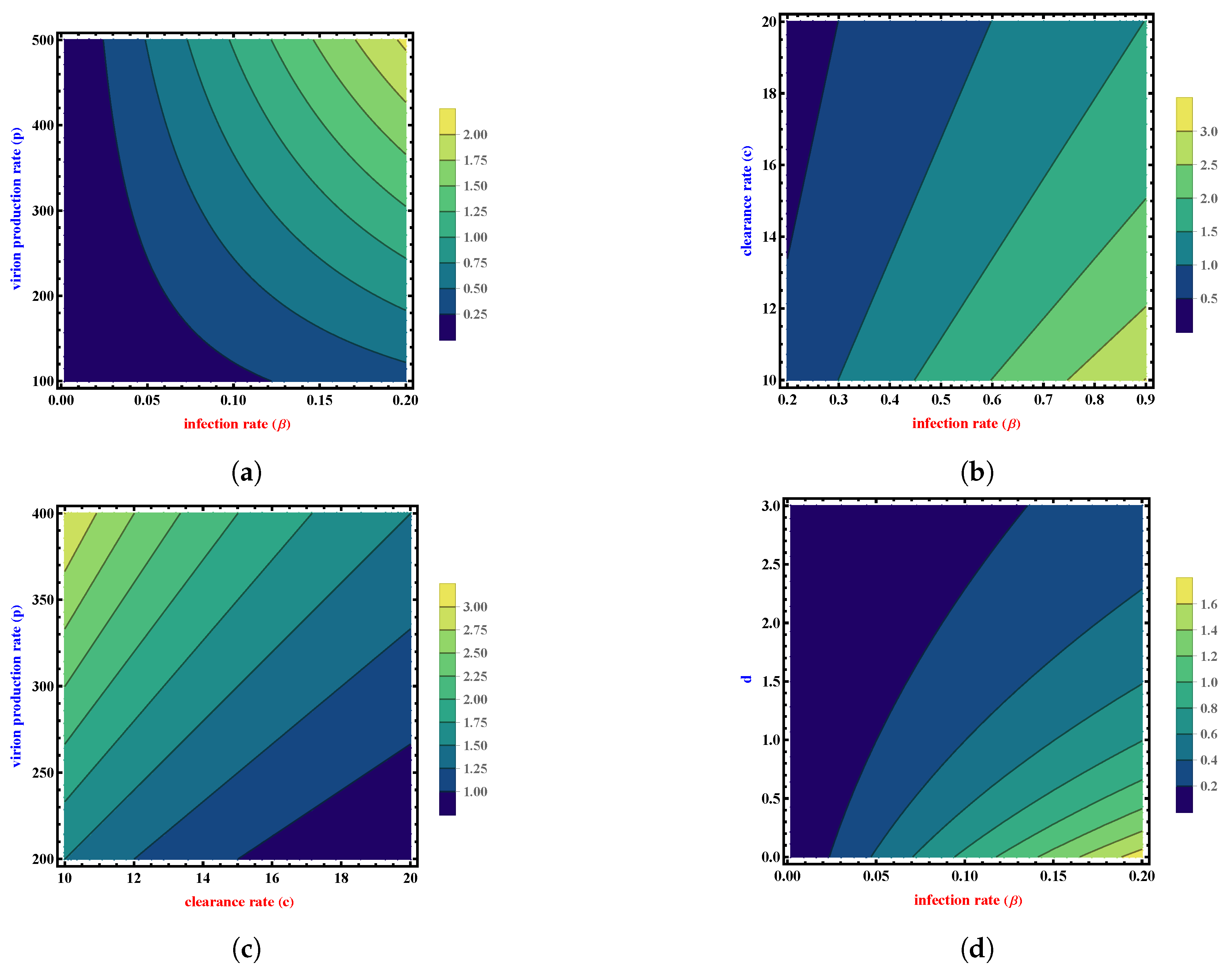
In Figure 5, we plot ${\mathfrak{R}}_0$ as a function of two important parameter of our model while keeping the rest of parameters constant.

Figure 5a suggests how ${\mathfrak{R}}_0$ increases as both p and $\beta$ rise. Figure 5b,c show the effect of increasing the clearance rate c: the basic reproduction number decreases with the rise of this parameter. ${\mathfrak{R}}_0$ becomes more sensitive to the clearance rate c. Ultimately, Figure 5d shows how ${\mathfrak{R}}_0$ becomes more sensitive to d as d decreases and $\beta$ increases.

6.3. Data Fitting

In order to validate our model, we fitted solutions of system (1) to actual data on Usutu virus titers based on experiments described by Heitzman-Breen et al. [15] and Kuchinsky et al. [41]. In these experiments, chicken were inoculated with different strains of Usutu virus and blood samples were collected from them for up to seven days post inoculation. For details of the experiments, see [15,41].

Methods applied during our fitting procedure include Latin hypercube sampling and least squares method. Latin hypercube sampling is a statistical sampling method which enables to generate a representative sample set of model parameters taking values from given parameter ranges [42]. Least squares method is a procedure often applied to approximate solutions by minimizing the sum of squares of the differences between the data points and the function values.

Solid blue lines in Figure 6 represent solution curves of model (1) using parameter values as described in

Table 3. Estimated parameter values of the model (1).

Parameter	(a)	(b)	(c)	(d)
$\mu$	1.26	0.64	0.002	0.36
d	0.43	0.44	0.07	0.43
$\beta$	$3\times {10}^{-3}$	${10}^{-3}$	$2\times {10}^{-3}$	$7\times {10}^{-3}$
k	1.36	1.35	1.41	0.81
$\delta$	24.13	10.27	3.3	2.5
p	422.1	372.1	16.16	8.83
c	17.18	16.8	10.22	16.03
$C_1$	3.48	4.89	6.93	7.14
$C_2$	4.24	1.22	9.71	9.82
$T\left(0\right)$	17.16	27.34	1869	18.94

, while red dots correspond to Usutu virus titer data points. Solution curves of our model pass through the viral load measurements providing a reasonably good fit for most data sets, suggesting that the model extended with cell birth and death can yield equally good (or sometimes even better) approximations of the virus data than the model without vital dynamics. At the same time, it has to be noted that in some cases, the model without cell birth and death gives a better result.

7. Discussion

Usutu virus, a pathogen affecting various bird species and occasionally causing spillover events in humans is among the emerging diseases deserving increased awareness. Despite the threat posed by the Usutu virus, not many mathematical models have been established to model this pathogen. In the present work, building upon the foundation established in [15], we set up and studied a within-host model for Usutu virus infection. To characterize interactions between healthy target cells, exposed cells, infected cells, and the viral particles, we built a mathematical model to capture the dynamics of Usutu virus within the host, incorporating the Crowley–Martin functional response and accounting for cell birth and death processes. By integrating the Crowley–Martin functional response, our model provides valuable insights into the complex interplay between Usutu virus and host cells, highlighting the pivotal role of host-virus interactions in shaping infection dynamics.

Examining the dynamic behavior of model (1), we completely described the global dynamics of the model and demonstrated that—depending on the parameters—the model has two possible equilibria, one disease-free and one infection equilibrium. Using the next generation matrix method, we calculated the basic reproduction number ${\mathfrak{R}}_0$. Constructing two appropriate Lyapunov functions, we found that the basic reproduction number ${\mathfrak{R}}_0$ serves as a threshold parameter and determines the model’s overall properties, with the disease-free equilibrium remaining stable if ${\mathfrak{R}}_0<1$ and the infection equilibrium being globally asymptotically stable if ${\mathfrak{R}}_0>1$. This means that if the basic reproduction number can be kept under the threshold value 1, the infection will be eradicated, while it will continue to persist otherwise. To assess the effectiveness of our model, numerical analysis was carried out. We performed sensitivity analysis on ${\mathfrak{R}}_0$ to study of the effect of varying different model parameters on the magnitude of the basic reproduction number, finding that the most influential parameters are cell birth rate and virus clearance rate, followed by infection rate, cell death rate and the virions’ production rate. We also fitted our model to actual data concerning Usutu virus titers. The fitting results suggest that our model including cell birth and death, as well as Crowley–Martin functional response is able to reproduce the dynamics of virus cells in most cases studied, moreover, the fitting is more precise than with a model without cell birth and death in several cases. However, it should be mentioned that in other cases, the model without cell birth and death provides a better fit. Our future work will follow the trajectory started in this paper, adding the spatial aspects to the model, creating a system of partial differential equations and better understanding the dynamics of viruses.

References

- Perelson, A.S.; Ribeiro, R.M. Modeling the within-host dynamics of HIV infection. BMC Biol. 2013, 11, 96. [Google Scholar] [CrossRef]
- Vaidya, N.K.; Bloomquist, A.; Perelson, A.S. Modeling within-host dynamics of SARS-CoV-2 infection: A case study in ferrets. Viruses 2021, 13, 1635. [Google Scholar] [CrossRef]
- Li, C.; Xu, J.; Liu, J.; Zhou, Y. The within-host viral kinetics of SARS-CoV-2. Math. Biosci. Eng. 2020, 17, 2853–2861. [Google Scholar] [CrossRef]
- Nikolay, B.; Diallo, M.; Boye, C.S.B.; Sall, A.A. Usutu virus in Africa. Vector-Borne Zoonotic Dis. 2011, 11, 1417–1423. [Google Scholar] [CrossRef]
- Gubler, D.J. The continuing spread of West Nile virus in the western hemisphere. Clin. Infect. Dis. 2007, 45, 1039–1046. [Google Scholar] [CrossRef]
- Clé, M.; Beck, C.; Salinas, S.; Lecollinet, S.; Gutierrez, S.; Van de Perre, P.; Simonin, Y. Usutu virus: A new threat? Epidemiol. Infect. 2019, 147, E232. [Google Scholar] [CrossRef]
- Chvala, S.; Kolodziejek, J.; Nowotny, N.; Weissenböck, H. Pathology and viral distribution in fatal Usutu virus infections of birds from the 2001 and 2002 outbreaks in Austria. J. Comp. Pathol. 2004, 131, 176–185. [Google Scholar] [CrossRef] [PubMed]
- Mossel, E.C.; Crabtree, M.B.; Mutebi, J.P.; Lutwama, J.J.; Borl, E.M.; Powers, A.M.; Miller, B.R. Arboviruses isolated from mosquitoes collected in Uganda, 2008–2012. J. Med. Entomol. 2017, 54, 1403–1409. [Google Scholar] [CrossRef] [PubMed]
- Dur, B.; Haskouri, H.; Lowenski, S.; Vachiéry, N.; Beck, C.; Lecollinet, S. Seroprevalence of West Nile and Usutu viruses in military working horses and dogs, Morocco, 2012: Dog as an alternative WNV sentinel species? Epidemiol. Infect. 2016, 144, 1857–1864. [Google Scholar]
- Hassine, T.B.; De Massis, F.; Calistri, P.; Savini, G.; BelHaj, M.B.; Ranen, A.; Di Gennaro, A.; Sghaier, S.; Hammami, S. First detection of co-circulation of West Nile and Usutu viruses in equids in the South-west of Tunisia. Transbound. Emerg. Dis. 2014, 61, 385–389. [Google Scholar] [CrossRef]
- Weissenböck, H.; Kolodziejek, J.; Url, A.; Lussy, H.; Rebel-Bauder, B.; Nowotny, N. Emergence of Usutu virus, an African mosquito-borne flavivirus of the Japanese encephalitis virus group, central Europe. Emerg. Infect. Dis. 2002, 8, 652. [Google Scholar] [CrossRef] [PubMed]
- Pecorari, M.; Longo, G.; Gennari, W.; Grottola, A.; Sabbatini, A.M.; Tagliazucchi, S.; Rumpianesi, F. First human case of Usutu virus neuroinvasive infection, Italy, August-September. Eurosurveillance 2009, 14, 19446. [Google Scholar] [CrossRef] [PubMed]
- Rubel, F.; Brugger, K. Dynamics of infectious diseases according to climate change: The Usutu virus epidemics in Vienna. In Game Meat Hygiene in Focus; Wageningen Academic Publishers: Wageningen, The Netherlands, 2011; pp. 173–198. [Google Scholar]
- Rubel, F.; Brugger, K.; Hantel, M.; Chvala-Mannsberger, S.; Bakonyi, T.; Weissenböck, H.; Nowotny, N. Explaining Usutu virus dynamics in Austria: Model development and calibration. Prev. Vet. Med. 2008, 85, 166–186. [Google Scholar] [CrossRef]
- Heitzman-Breen, N.; Golden, J.; Vazquez, A.; Kuchinsky, S.C.; Duggal, N.K.; Ciupe, S.M. Modeling the dynamics of Usutu virus infection of birds. J. Theor. Biol 2021, 531, 110896. [Google Scholar] [CrossRef]
- Weissenböck, H.; Kolodziejek, J.; Fragner, K.; Kuhn, R.; Pfeffer, M.; Nowotny, N. Usutu virus activity in Austria, 2001–2002. Microbes Infect. 2003, 5, 1132–1136. [Google Scholar] [CrossRef] [PubMed]
- Bakonyi, T.; Gould, E.A.; Kolodziejek, J.; Weissenböck, H.; Nowotny, N. Complete genome analysis and molecular characterization of Usutu virus that emerged in Austria in 2001: Comparison with the South African strain SAAR-1776 and other flaviviruses. Virology 2004, 328, 301–310. [Google Scholar]
- Bakonyi, T.; Lussy, H.; Weissenböck, H.; Hornyák, Á.; Nowotny, N. In vitro host-cell susceptibility to Usutu virus. Emerg. Infect. Dis. 2005, 11, 298. [Google Scholar] [CrossRef]
- Yang, Y. Global analysis of a virus dynamics model with general incidence function and cure rate. Abstr. Appl. Anal. 2014, 2014, 726349. [Google Scholar] [CrossRef]
- Wang, J.; Zhang, R.; Kuniya, T. Global dynamics for a class of age-infection HIV models with nonlinear infection rate. J. Math. Anal. Appl. 2015, 432, 289–313. [Google Scholar] [CrossRef]
- Crowley, P.H.; Martin, E.K. Functional responses and interference within and between year classes of a dragonfly population. J. N. Am. Benthol. Soc. 1989, 8, 211–221. [Google Scholar] [CrossRef]
- Meng, X.Y.; Huo, H.F.; Xiang, H.; Yin, Q.Y. Stability in a predator–prey model with Crowley–Martin function and stage structure for prey. Appl. Math. Comput. 2014, 232, 810–819. [Google Scholar] [CrossRef]
- Li, X.; Lin, X.; Liu, J. Existence and global attractivity of positive periodic solutions for a predator-prey model with Crowley-Martin functional response. Electron. J. Differ. Equ. 2018, 191, 1–17. Available online: https://digital.library.txstate.edu/handle/10877/15487 (accessed on 1 June 2023).
- Hattaf, K.; Yousfi, N.; Tridane, A. Global stability analysis of a generalized virus dynamics model with the immune response. Can. Appl. Math. Q. 2012, 20, 499–518. [Google Scholar]
- Zhou, X.; Cui, J. Global stability of the viral dynamics with Crowley-Martin functional response. Bull. Korean Math. Soc. 2011, 48, 555–574. [Google Scholar] [CrossRef]
- Xu, S. Global stability of the virus dynamics model with Crowley–Martin functional response. Electron. J. Qual. Theory Differ. Equ. 2012, 2012, 1–10. [Google Scholar] [CrossRef]
- Li, X.; Fu, S. Global stability of the virus dynamics model with intracellular delay and Crowley–Martin functional response. Math. Methods Appl. Sci. 2014, 37, 1405–1411. [Google Scholar] [CrossRef]
- Wang, S.; Song, X. Global properties for an age-structured within-host model with Crowley–Martin functional response. Int. J. Biomath. 2017, 10, 1750030. [Google Scholar] [CrossRef]
- De Madrid, A.T.; Porterfield, J.S. The flaviviruses (group B arboviruses): A cross-neutralization study. J. Gen. Virol. 1974, 23, 91–96. [Google Scholar] [CrossRef] [PubMed]
- Diekmann, O.; Heesterbeek, J.A.P.; Roberts, M.G. The construction of next-generation matrices for compartmental epidemic models. J. R. Soc. Interface 2010, 7, 873–885. [Google Scholar] [CrossRef] [PubMed]
- Clark, R.N. The Routh-Hurwitz stability criterion, revisited. IEEE Control. Syst. Mag. 1992, 12, 119–120. [Google Scholar]
- Bodson, M. Explaining the Routh–Hurwitz Criterion: A Tutorial Presentation [Focus on Education]. IEEE Control. Syst. Mag. 2020, 40, 45–51. [Google Scholar] [CrossRef]
- Wang, K.; Jin, Y.; Fan, A. The effect of immune responses in viral infections: A mathematical model view. Discret. Contin. Dyn.-Syst.-B 2014, 19, 3379. [Google Scholar] [CrossRef]
- Vargas-De-León, C. Constructions of Lyapunov functions for classic SIS, SIR and SIRS epidemic models with variable population size. Foro-Red-Mat. Rev. Electrónica Conten. Matemático 2009, 26, 1–12. [Google Scholar]
- Wang, X.; Tao, Y.; Song, X. Global stability of a virus dynamics model with Beddington–DeAngelis incidence rate and CTL immune response. Nonlinear Dyn. 2011, 66, 825–830. [Google Scholar] [CrossRef]
- Gao, D.P.; Huang, N.J.; Kang, S.M.; Zhang, C. Global stability analysis of an SVEIR epidemic model with general incidence rate. Bound. Value Probl. 2018, 2018, 42. [Google Scholar] [CrossRef]
- Hattaf, K.; Yousfi, N. Dynamics of SARS-CoV-2 infection model with two modes of transmission and immune response. Math. Biosci. Eng. 2020, 17, 5326–5340. [Google Scholar] [CrossRef]
- Elaiw, A.M.; Alade, T.O.; Alsulami, S.M. Global stability of within-host virus dynamics models with multitarget cells. Mathematics 2018, 6, 118. [Google Scholar] [CrossRef]
- Zhang, T.; Meng, X.; Zhang, T. Global dynamics of a virus dynamical model with cell-to-cell transmission and cure rate. Comput. Math. Methods Med. 2015. [Google Scholar] [CrossRef] [PubMed]
- Huang, G.; Ma, W.; Takeuchi, Y. Global properties for virus dynamics model with Beddington–DeAngelis functional response. Appl. Math. Lett. 2009, 22, 1690–1693. [Google Scholar] [CrossRef]
- Kuchinsky, S.C.; Frere, F.; Heitzman-Breen, N.; Golden, J.; Vázquez, A.; Honaker, C.F.; Siegel, P.B.; Ciupe, S.M.; LeRoith, T.; Duggal, N.K. Pathogenesis and shedding of Usutu virus in juvenile chickens. Emerg. Microbes Infect. 2021, 10, 725–738. [Google Scholar] [CrossRef] [PubMed]
- McKay, M.D.; Beckman, R.J.; Conover, W.J. A comparison of three methods for selecting values of input variables in the analysis of output from a computer code. Technometrics 1979, 21, 239–245. [Google Scholar]
Figure 1.
Virus transmission cycle: from reservoir host to vector, onward to avian hosts. ’Dead end’ hosts like horses or humans, where the virus transmission is limited are also highlighted.
Figure 2.
Flow chart of the infection dynamics of Usutu virus. (shown in blue) stands for healthy target cells, (shown in orange) denotes exposed cells, (shown in green) stands for infected cells. Virus particles () are shown in red. The meaning of the parameters is given in Table 1.
Figure 3.
Solution curves of system (1) illustrating the dynamics for different values of : (a) depicting disease extinction, and (b) showing disease persistence.
Figure 4.
Partial rank correlation coefficients of parameters of model (1).
Figure 5.
Contour plots of the basic reproduction number for various parameter values. (a) Contour plot of as a function of and p. (b) Contour plot of as a function of and c. (c) Contour plot of as a function of c and p. (d) Contour plot of as a function of and d.
Figure 6.
Virus curve (blue line) represents the model (1) prediction, while the red dots indicate the experimental data points, with a confidence interval, which was obtained by letting for all parameters a 5% relative error with respect to the best fitting values. Parameter values are given in Table 3. For details of the experiments, see [15,41]. Subfigures correspond to the following experiments in [15]: (a) B7 (b) B16 (c) B25 (d) B31.