Application of Orthogonal Functions to Equivalent Linearization Method for MDOF Duffing–Van der Pol Systems under Nonstationary Random Excitations

Abstract

Many mechanical systems manifest nonlinear behavior under nonstationary random excitations. Neglecting this nonlinearity in the modeling of a dynamic system would result in unacceptable results. However, it is challenging to find exact solutions to nonlinear problems. Therefore, equivalent linearization methods are often used to seek approximate solutions for this kind of problem. To overcome the limitations of the existing equivalent linearization methods, an orthogonal-function-based equivalent linearization method in the time domain is proposed for nonlinear systems subjected to nonstationary random excitations. The proposed method is first applied to a single-degree-of-freedom (SDOF) Duffing–Van der Pol oscillator subjected to stationary and nonstationary excitations to validate its accuracy. Then, its applicability to nonlinear MDOF systems is depicted by a 5DOF Duffing–Van der Pol system subjected to nonstationary excitation, with different levels of system nonlinearity strength considered in the analysis. Results show that the proposed method has the merit of predicting the nonlinear system response with high accuracy and computation efficiency. In addition, it is applicable to any general type of nonstationary random excitation.

1. Introduction

Many physical and mechanical systems manifest nonlinear behavior under nonstationary excitations, which must be taken into account in the analysis and design to avoid misleading and unacceptable results. While linear dynamic problems can typically be solved using standard analytical approaches in both time and frequency domains, tackling nonlinear systems subjected to nonstationary excitations is much more challenging. A number of effective methods, such as the perturbation method [1], the Fokker–Planck–Kolmogorov (FPK) equation method [2], the moment equation method [3], the equivalent linearization (EL) method [4] and the Monte Carlo (MC) simulation method [5], have been developed to conduct random vibration analyses of nonlinear systems. Although exact analytical solutions to some particular nonlinear dynamic problems have been found using the FPK method [2], it is generally not available in many practical problems. Consequently, using approximation methods to determine the response of nonlinear dynamic systems resulting from random nonstationary excitations becomes necessary. Among various available approximation methods, the equivalent linearization (EL) method and the Monte Carlo (MC) simulation method are more popular due to their applicability to multi-degree-of-freedom (MDOF) systems and nonstationary excitation problems. The MC simulation method involves a large number of sample tests and is thus very expensive in computational cost. Hence, it is often used as a benchmark for other methods. The EL methods do not have these restrictions and have broad applications. In general, this technique consists of two main steps. The first step requires finding analytical formulas for linearization coefficients, which are based on the linearization criterion dependent on unknown response statistical terms such as variance and higher-order moments. The actual set of nonlinear equations is then replaced by an equivalent linear set for the solution. In the EL methods, the coefficients of the equivalent system can be found based on a specified optimization criterion in some probabilistic sense, such as the mean square criterion [4], the spectral criteria [6], the probability density criteria [7] and the energy criteria [8].

Nonstationary excitations typically originate from uncertain transient loading conditions, such as wind, earthquake and blast excitation. Although the nonstationary problems attract much interest, the analysis of nonstationary responses of nonlinear systems has not been fully explored due to the complexity of the problem. An analytical approach for SDOF nonlinear systems with parameter uncertainty subjected to nonstationary excitation was proposed by Huang and Iwan [9], where a set of orthogonal polynomials associated with the probability density function was used as the solution basis for the response moments. In 1987, Orabi and Ahmadi [10] studied a single-degree-of-freedom (SDOF) nonlinear system under particular types of nonstationary excitations using the equivalent linearization method. In addition, a new approach has been proposed for simulating rotational components of earthquake excitation in terms of translational independent components and TELM has been applied for a 3D structure considering rotational components of earthquakes. A numerical example shows the abilities of the tail equivalent linearization method in predicting the probabilities of failure in comparison with simulation results [11]. Ma et al. [12] used the pseudo-excitation method to obtain the solution to the nonstationary random responses of MDOF nonlinear systems.

In practical applications, it is vital to precisely capture the behavior of nonlinear systems under excitations possessing inherent nonstationary characteristics. However, most of the existing methods can be computationally prohibitive in dealing with this kind of problem, especially when large-scale nonlinear systems are involved. They are either incapable of directly solving the system equation of motion or only focus on specific types of external excitation and cannot be applied to more general loading cases. The stochastic equivalent linearization (EL) method is one of the most popular approximate solutions for nonlinear systems [13], but the implementation of this approach by numerical techniques would be demanding. Recently, a number of researchers addressed this issue in the time domain. In particular, Su and Xu [14] developed and applied an explicit time domain approach to different random vibration problems associated with linear structures under nonstationary excitations. Moreover, an explicit time domain method by using the direct differentiation method has been proposed in [15]. An efficient approach by combining the time domain explicit formulation method and the EL method for the random vibration analysis of nonlinear MDOF structures subjected to nonstationary random excitations was developed by Su et al. [16], except the formulation of the approach requires the provision of the cross-correlation functions of the excitations in order to compute the correlation matrix of the displacement vector to obtain the second-order moment of response. This requirement would be challenging to satisfy in the case of general nonstationary random excitations, such as seismic load. Therefore, there is an urgent need to develop an alternative EL method in the time domain to accurately and efficiently predict the response of nonlinear systems subjected to any type of general nonstationary random excitation. This is achieved in the current study by introducing the orthogonal functions in the equivalent linearization.

The orthogonal functions have been extensively used in the numerical analysis and approximation theory of various engineering problems to improve the accuracy of the approximated responses and reduce the computational cost. For structural applications, the orthogonal functions may be classified into three families, including the piecewise constant orthogonal functions, the orthogonal polynomials and the Fourier functions [17]. These functions have been effective tools for the analysis of dynamic systems since the 1970s [18]. The application of these functions to controlling systems, as well as to system identification and sensitivity analysis, can be found in some recent studies [19,20,21,22,23,24]. If an orthogonal function is converted to an orthonormal one, it would not only further improve the approximation accuracy, but also simplify the mathematical operation. Among various orthogonal functions, the block pulse (BP) functions, which are a set of orthogonal functions with a unit pulse at each time step, are inherently orthonormal. They are capable of reducing the original problem to the solution of a set of complex algebraic equations, which is thus computationally more efficient.

The existing equivalent linearization methods are mostly limited to the nonlinear systems with low to moderate nonlinearity and are applicable to stationary or particular types of nonstationary excitation. The focus of the current study is to develop an orthogonal-function-based equivalent linearization method in the time domain for analyzing MDOF nonlinear systems with strong nonlinearity under nonstationary excitations, with the BP function applied to the equivalent linearization procedure. In the proposed method, the statistical moments of the nonstationary system responses can be directly determined in the time domain and there is no need to convert the response to the frequency domain, which is necessary in some available techniques. Thus, the proposed approach is more efficient when compared to the mixed time–frequency domain methods, in which a large number of time–history integrals are required at different frequency intervals when nonstationary random excitations are involved. Even in complex MDOF systems, this approach is capable of achieving rapid convergence. Further, the formulation of the proposed approach allows it to be applicable to more general and realistic types of nonstationary excitation, such as seismic load. An SDOF nonlinear Duffing–Van der Pol oscillator under both stationary and nonstationary excitations is considered first to evaluate the validity of the proposed method. Results show that the proposed method is more accurate than the existing approaches. Although the required time for satisfying the convergence requirement by the proposed method was almost the same as the other existing EL approaches, fewer iterations were needed by the proposed approach. The applicability of the proposed method to MDOF nonlinear systems under nonstationary excitation is demonstrated by a 5DOF Duffing–Van der Pol nonlinear system. The computational advantage of the proposed approach is even more predominant in analyzing MDOF nonlinear systems, of which the computational time required for solving nonstationary excitation problems was considerably less. The remainder of this paper is organized as follows: a review of the orthogonal functions is presented in Section 2. Section 3 illustrates the equivalent linearization process using the orthogonal functions. For comparison, case studies are carried out in Section 4. Highlighting of the contributions and summarizing of the main findings appear in Section 5.

2. Review of Orthogonal Functions

A set of functions ${\varphi }_i\left(t\right)(i=1,2,3,\dots )$ is said to be orthogonal over the interval $[a,b]$ if

$${\int }_a^b{\varphi }_m\left(t\right){\varphi }_n\left(t\right)dt=K_{mn}$$

(1)

where $K_{mn}$ is a nonzero positive constant, which satisfies

$$\left\{\begin{array}{c}{K}_{mn}=0\hspace{1em}\mathrm{i}\mathrm{f}\hspace{1em}\mathrm{m}\ne \mathrm{n}\\ K_{mn}\ne 0\hspace{1em}\mathrm{i}\mathrm{f}\hspace{1em}\mathrm{m}=\mathrm{n}\end{array}\right.$$

If $K_{mn}$ is the Kronecker delta function, the set of functions ${\varphi }_i\left(t\right)$ is said to be orthonormal. The following property, related to the successive integration of the vectorial basis, holds for a set of $r$ orthonormal functions:

$$\underset{n times}{\underbrace{{\int }_0^t\dots {\int }_0^t\left\{\varphi \left(\tau \right)\right\}{\left(d\tau \right)}^n}}\cong {\left[P\right]}^n\left\{\varphi \left(t\right)\right\}$$

(2)

where $\left[P\right]\in {\mathfrak{R}}^{r,r}$ is a square matrix with constant elements, which is called an operator or operational matrix and is dependent on the type of orthogonal function and $\left\{\varphi \left(t\right)\right\}={[{\varphi }_0\left(t\right),{\varphi }_1\left(t\right),\dots ,{\varphi }_{r-1}\left(t\right)]}^T$ is the vectorial basis of the orthonormal series. This operator plays a key role in the methodology. The operators give a proper mathematical frame for the orthogonal functions and are advantageous to the convergence analysis of their series expansions. In other words, the operators would produce an image matrix or vector of function $f\left(t\right)$ in the orthogonal function domain.

A set of BP functions over a unit time interval $\left[0,1\right)$ is defined as [25]:

$${\varphi }_i\left(t\right)=\left\{\begin{array}{cc}1& \frac{i}{m}\le t\le \frac{i+1}{m}\\ 0& otherwise\end{array}\right.$$

(3)

where $i=0,1,2,\dots ,m-1$ where $m$ is a positive integer value, and ${\varphi }_i$ is the i-th BP function.

The block pulse operator $\mathcal{B}$ is determined in the BP domain as

$$\mathcal{B}\left\{f\left(t\right)\right\}=F^T$$

(4)

where vector $F$ is evaluated from

$$F=\frac{1}{q}{\int }_0^{T}f\left(t\right)\varphi \left(t\right)dt=[f_1,f_2,\dots ,f_m]$$

(5)

where $q=1/m$. The BP operator has numerous operation rules, of which those that are applied in the next section are listed below [25].

(a)

For a real constant k, we have

$$\mathcal{B}\left\{k\right\}=k{E}^T$$

(6)

where $E^T$ is a constant vector with all entries being one.

(b)

For addition and subtraction of functions $f\left(t\right)$, $g\left(t\right)\in [0,T)$, we have:

$$\mathcal{B}\left\{f\left(t\right)\pm g\left(t\right)\right\}=F^T\pm G^T$$

(7)

This relation can be derived directly from the linearity of the BP operator.

(c)

For integration of a function $f\left(t\right)\in [0,T)$, we have

$$\mathcal{B}\left\{{\int }_0^{T}f\left(t\right)dt\right\}=F^{T}P$$

(8)

where $P$ is a conventional integration operational matrix defined as

$$P=\frac{q}{2}\left[\begin{array}{ccccc}1& 2& 2& \cdots & 2\\ 0& 1& 2& \cdots & 2\\ 0& 0& 1& \cdots & 2\\ ⋮& ⋮& ⋮& \ddots & ⋮\\ 0& 0& 0& ⋮& 1\end{array}\right]$$

(9)

(d)

For convolution integral of functions $f\left(t\right)$, $g\left(t\right)\in [0,T)$, we have:

$$\mathcal{B}\left\{{\int }_0^{T}f\left(\tau \right)g(t-\tau )d\tau \right\}\cong {\frac{q}{2}F}^T{J}_G\cong {\frac{q}{2}G}^T{J}_F$$

(10)

where $J_G$ and $J_F$ are the convolution operational matrices defined in Equations (11) and (12).

$$J_F=\frac{q}{2}\left[\begin{array}{ccc}{f}_1& f_1+f_2& \begin{array}{ccc}{f}_2+f_3& \cdots & f_{m-1}+f_m\end{array}\\ 0& f_1& \begin{array}{ccc}{f}_1+f_2& \cdots & f_{m-2}+f_{m-1}\end{array}\\ \begin{array}{c}0\\ ⋮\\ 0\end{array}& \begin{array}{c}0\\ ⋮\\ 0\end{array}& \begin{array}{ccc}\begin{array}{c}{f}_1\\ ⋮\\ 0\end{array}& \begin{array}{c}\cdots \\ \ddots \\ \cdots \end{array}& \begin{array}{c}{f}_{m-3}+f_{m-2}\\ ⋮\\ f_1\end{array}\end{array}\end{array}\right]$$

(11)

$$J_G=\frac{q}{2}\left[\begin{array}{ccc}{g}_1& g_1+g_2& \begin{array}{ccc}{g}_2+g_3& \cdots & g_{m-1}+g_m\end{array}\\ 0& g_1& \begin{array}{ccc}{g}_1+g_2& \cdots & g_{m-2}+g_{m-1}\end{array}\\ \begin{array}{c}0\\ ⋮\\ 0\end{array}& \begin{array}{c}0\\ ⋮\\ 0\end{array}& \begin{array}{ccc}\begin{array}{c}{g}_1\\ ⋮\\ 0\end{array}& \begin{array}{c}\cdots \\ \ddots \\ \cdots \end{array}& \begin{array}{c}{g}_{m-3}+g_{m-2}\\ ⋮\\ g_1\end{array}\end{array}\end{array}\right]$$

(12)

(e)

For multiple integrals, we have the following rule:

$$\mathcal{B}\left\{\underset{k}{\underbrace{{\int }_0^t\dots {\int }_0^{t}f\left(t\right)dt\cdots dt}}\right\}=F^T{P}^k$$

(13)

3. The Equivalent Linearization Technique Based on Orthogonal Functions

3.1. SDOF System

The equation of motion of an SDOF nonlinear system is given as

$$\ddot{x}\left(t\right)+2\beta \dot{x}\left(t\right)+{\omega }^{2}x\left(t\right)+g\left[x\left(t\right),\dot{x}\left(t\right)\right]=w\left(t\right)$$

(14)

with

$$\beta =\xi \omega$$

(15)

where $\xi$ and $\omega$ are, respectively, the damping coefficient and the system frequency, $x\left(t\right), \dot{x}\left(t\right)$ and $\ddot{x}\left(t\right)$ are, respectively, the displacement, the velocity and the acceleration vectors, $g\left[x\left(t\right),\dot{x}\left(t\right)\right]$ is a nonlinear function of displacement and velocity, $w\left(t\right)$ is the excitation, which is assumed to be a zero-mean nonstationary random process.

In accord with the equivalent linearization method, Equation (14) can be replaced by the following equation of motion as

$$\ddot{y}\left(t\right)+2{\beta }_{eq}\dot{y}\left(t\right)+{\omega }_{eq}^{2}y\left(t\right)=w\left(t\right)$$

(16)

where the coefficients of linearization, ${\beta }_{eq}$ and ${\omega }_{eq}$, can be found by the equivalent linearization approach. If the excitation to the original nonlinear system is a Gaussian function, the response of the equivalent linear system will also be Gaussian. Therefore, the equivalent linearization coefficients can be calculated by the simplified expressions proposed by Atalik and Utku [26].

The coefficients ${\beta }_{eq}$ and ${\omega }_{eq}$ are determined as follows:

$${2\beta }_{eq}=2\beta +E\left[\frac{\partial g(x,\dot{x})}{\partial \dot{x}}\right]$$

(17)

$${\omega }_{eq}^2={\omega }^2+E\left[\frac{\partial g(x,\dot{x})}{\partial x}\right]$$

(18)

where $E[.]$ stands for the mathematical expectation.

For nonstationary analysis, the equivalent damping and frequency are functions of time. For a system which is initially at rest ($x\left(0\right)=\dot{x}\left(0\right)=0$) and by assuming that these coefficients are constants as in stationary analysis, the solution to Equation (16) in the time domain can be expressed by the Duhamel integral as follows:

$$x\left(t\right)={\int }_{-\infty }^{\infty }h\left({\tau }_1\right)w\left(t-{\tau }_1\right)d{\tau }_1={\int }_{-\infty }^{\infty }h\left(t-{\tau }_1\right)w\left({\tau }_1\right)d{\tau }_1$$

(19)

where $h\left(t\right)$ is the impulse response of the linearized system and is defined as follows:

$$h\left(t\right)=\left\{\begin{array}{ccc}\frac{1}{{\omega }_d}{e}^{-{\beta }_{eq}t}\sin ({\omega }_{d}t)& ;\hspace{1em}& t\ge 0\\ 0\hspace{1em}& ;\hspace{1em}& t<0\end{array}\right.$$

(20)

where

$${\omega }_d^2={\omega }_{eq}^2-{\beta }_{eq}^2$$

(21)

Using Equation (19) to evaluate the mean square response or variance of the displacement and velocity responses gives [27]

$$E\left[x^2\right]=\underset{-\infty }{\overset{\infty }{\iint }}h\left(t-{\tau }_1\right)w\left({\tau }_1\right)w\left({\tau }_2\right)h(t-{\tau }_2)d{\tau }_{1}d{\tau }_2$$

(22)

$$E\left[{\dot{x}}^2\right]=\underset{-\infty }{\overset{\infty }{\iint }}\dot{h}\left(t-{\tau }_1\right)w\left({\tau }_1\right)w\left({\tau }_2\right)\dot{h}(t-{\tau }_2)d{\tau }_{1}d{\tau }_2$$

(23)

The linearization coefficients can be determined by using the values calculated from Equations (22) and (23). The solution of the mean square response as given is valid for constant values of ${\beta }_{eq}$ and ${\omega }_{eq}$. However, as is obvious from Equations (17) and (18), the equivalent damping and frequency are, in general, functions of time in the nonstationary random process. Using the constant stationary limits with long duration for these coefficients is a usual assumption. However, this assumption gives first-order approximate solutions for the nonstationary responses. To overcome this limitation, an iterative solution procedure is introduced to improve the accuracy of the solutions (see [10,28]).

• Assign initial estimations of $c_{eq}$ and $k_{eq}$ in order to obtain the mean square response of displacement and velocity ($E\left[x^2\right]$, $E\left[{\dot{x}}^2\right]$).
• Substitute the obtained values into Equations (17) and (18) to obtain new estimations for ${\beta }_{eq}$ and ${\omega }_{eq}$.
• In order to find new estimation for the mean square response, substitute the new values of ${\beta }_{eq}$ and ${\omega }_{eq}$ into Equation (20) and then Equations (22) and (23).
• Use the obtained $E\left[x^2\right]$ and $E\left[{\dot{x}}^2\right]$ values and return to step (2).
• Repeat steps (2), (3) and (4) until the results satisfy the following convergence criterion:

  $$\frac{E{\left[x^2\right]}_{i+1}-E{\left[x^2\right]}_i}{E{\left[x^2\right]}_i}<\epsilon ; \frac{E{\left[{\dot{x}}^2\right]}_{i+1}-E{\left[{\dot{x}}^2\right]}_i}{E{\left[{\dot{x}}^2\right]}_i}<\epsilon$$

  (24)

  where $\epsilon =0.001$ was used in the current study.

To reduce the computational complexity, the mean square response of the linearized system is calculated using the operational rules of orthogonal functions in this paper, i.e., Equations (10)–(13). By applying the convolution integral (Equation (10)) and the multiple integral (Equation (13)) operators of the BP functions, we have:

$$\begin{array}{l}E\left[x^2\right]=\underset{-\infty }{\overset{\infty }{\iint }}h\left(t-{\tau }_1\right)w\left({\tau }_1\right)w\left({\tau }_2\right)h(t-{\tau }_2)d{\tau }_{1}d{\tau }_2\\ ={\int }_{-\infty }^{\infty }{h}^2\left(t-\tau \right)w^2\left(\tau \right)d\tau ={\int }_{-\infty }^{\infty }r\left(t-\tau \right)w^2\left(\tau \right)d\tau ={\frac{q^2}{4}R}^T{J_w}^2\\ =\frac{q^2}{4}[r_1,r_2,\dots ,r_m]{\left[\begin{array}{ccc}{w}_1& w_1+w_2& \begin{array}{ccc}{w}_2+w_3& \cdots & w_{m-1}+w_m\end{array}\\ 0& w_1& \begin{array}{ccc}{w}_1+w_2& \cdots & w_{m-2}+w_{m-1}\end{array}\\ \begin{array}{c}0\\ ⋮\\ 0\end{array}& \begin{array}{c}0\\ ⋮\\ 0\end{array}& \begin{array}{ccc}\begin{array}{c}{w}_1\\ ⋮\\ 0\end{array}& \begin{array}{c}\cdots \\ \ddots \\ \cdots \end{array}& \begin{array}{c}{w}_{m-3}+w_{m-2}\\ ⋮\\ w_1\end{array}\end{array}\end{array}\right]}^2\end{array}$$

(25)

where ${r\left(t-\tau \right)=h}^2\left(t-\tau \right)$ and

$$r_i=\frac{1}{q}{\int }_{iq}^{\left(i+1\right)q}r\left(t\right)\varphi \left(t\right)dt;\hspace{1em}{w}_i=\frac{1}{q}{\int }_{iq}^{\left(i+1\right)q}w\left(t\right)\varphi \left(t\right)dt$$

(26)

and

$$\begin{array}{l}E\left[{\dot{x}}^2\right]=\underset{-\infty }{\overset{\infty }{\iint }}\dot{h}\left(t-{\tau }_1\right)w\left({\tau }_1\right)w\left({\tau }_2\right)\dot{h}(t-{\tau }_2)d{\tau }_{1}d{\tau }_2\\ ={\int }_{-\infty }^{\infty }{\dot{h}}^2\left(t-\tau \right)w^2\left(\tau \right)d\tau ={\int }_{-\infty }^{\infty }l\left(t-\tau \right)w^2\left(\tau \right)d\tau ={\frac{q^2}{4}L}^T{J_w}^2\\ =\frac{q^2}{4}[l_1,l_2,\dots ,l_m]{\left[\begin{array}{ccc}{w}_1& w_1+w_2& \begin{array}{ccc}{w}_2+w_3& \cdots & w_{m-1}+w_m\end{array}\\ 0& w_1& \begin{array}{ccc}{w}_1+w_2& \cdots & w_{m-2}+w_{m-1}\end{array}\\ \begin{array}{c}0\\ ⋮\\ 0\end{array}& \begin{array}{c}0\\ ⋮\\ 0\end{array}& \begin{array}{ccc}\begin{array}{c}{w}_1\\ ⋮\\ 0\end{array}& \begin{array}{c}\cdots \\ \ddots \\ \cdots \end{array}& \begin{array}{c}{w}_{m-3}+w_{m-2}\\ ⋮\\ w_1\end{array}\end{array}\end{array}\right]}^2\end{array}$$

(27)

where ${l\left(t-\tau \right)=\dot{h}}^2\left(t-\tau \right)$ and

$$l_i=\frac{1}{q}{\int }_{iq}^{\left(i+1\right)q}l\left(t\right)\varphi \left(t\right)dt$$

(28)

3.2. MDOF System

The equation of motion of an n-degree-of-freedom nonlinear system is given as

$$\mathit{M}\ddot{\mathit{x}}\left(t\right)+\mathit{C}\dot{\mathit{x}}\left(t\right)+\mathit{K}\mathit{x}\left(t\right)+\mathit{G}(\mathit{x}\left(t\right),\dot{\mathit{x}}(t\left)\right)=\mathit{\varphi }\mathit{W}\left(t\right)$$

(29)

where $\mathit{M}, \mathit{C}$ and $\mathit{K}$ are the $n\times n$ mass matrix, damping matrix and elastic stiffness matrix of the considered system, respectively; $\mathit{x}\left(t\right), \dot{\mathit{x}}\left(t\right)$ and $\ddot{\mathit{x}}\left(t\right)$ denote the nodal displacement vector and the corresponding velocity vector and acceleration vector, respectively; $\mathit{G}\left(\mathit{x}\left(t\right),\dot{\mathit{x}}\left(t\right)\right)={\left[g_1\right(t\left)g_2\right(t)\dots g_n(t\left)\right]}^T$ is an n-dimension nonlinear vector function of the coordinate displacement and velocity, $\mathit{\varphi }$ is an orientation matrix of the nonstationary zero-mean Gaussian random loading vector $W\left(t\right)={[W_1\left(t\right)W_2\left(t\right)\dots W_n(t\left)\right]}^T$, where the superscript T denotes matrix transposition.

By assuming linear behavior for the mass matrix, Equation (29) can be replaced by the following equivalent linear equation of motion as

$$\mathit{M}\ddot{\mathit{x}}\left(t\right)+\left[\mathit{C}+{\mathit{C}}_{\mathit{e}\mathit{q}}\left(\tau \right)\right]\dot{\mathit{x}}\left(t\right)+\left[\mathit{K}+{\mathit{K}}_{\mathit{e}\mathit{q}}\left(\tau \right)\right]\mathit{x}\left(t\right)=\mathit{\varphi }\mathit{W}\left(t\right)$$

(30)

where ${\mathit{C}}_{\mathit{e}\mathit{q}}\left(\tau \right)$ and ${\mathit{K}}_{\mathit{e}\mathit{q}}\left(\tau \right)$ are, respectively, the $n\times n$ equivalent matrices at time instant $\tau$. By assuming the Gaussian excitation and using the simplified expressions proposed in [26], the elements of the equivalent linearization matrices can be obtained by the following equations:

$$K_{eq,ij}\left(\tau \right)=E\left[\frac{\partial g_i\left(\tau \right)}{\partial x_j\left(\tau \right)}\right]\hspace{1em}i,j=1,2,\dots ,n$$

(31)

$$C_{eq,ij}\left(\tau \right)=E\left[\frac{\partial g_i\left(\tau \right)}{\partial {\dot{x}}_j\left(\tau \right)}\right]\hspace{1em}i,j=\mathrm{1,2},\dots ,n$$

(32)

where $K_{eq,ij}\left(\tau \right)$ and $C_{eq,ij}\left(\tau \right)$ are the elements of ${\mathit{K}}_{\mathit{e}\mathit{q}}\left(\tau \right)$ and ${\mathit{C}}_{\mathit{e}\mathit{q}}\left(\tau \right)$, respectively. It is evident that the equivalent parameters in Equations (31) and (32) depend on the statistical responses. Therefore, an iterative procedure proposed in the previous section is required to determine the accurate equivalent matrices.

Again, we assume that the considered MDOF system would be initially at rest. By conducting modal analysis, the solution to every degree of freedom (Equation (30)) in the time domain can be evaluated using Equations (19)–(23). Therefore, in the case of an MDOF system, the concept of orthogonal functions can be used to approximate the linearization coefficients, and the mean square values of the system response. In the next section, the proposed method will be applied to examples of SDOF and MDOF systems subjected to nonstationary random excitations.

4. Numerical Examples

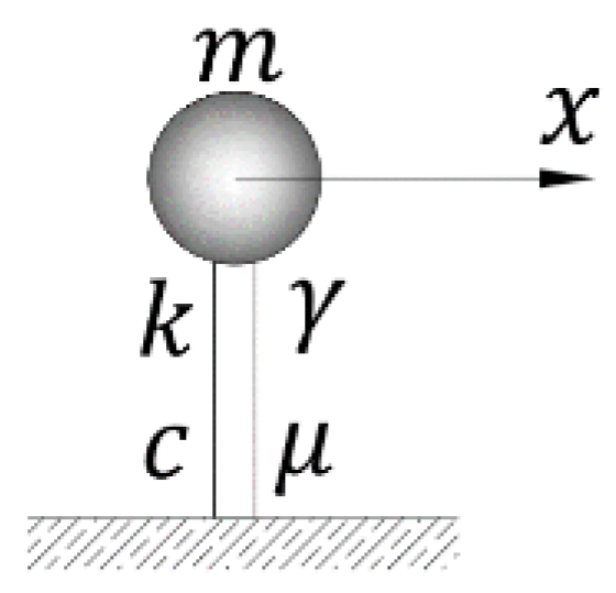
4.1. SDOF Duffing–Van der Pol Oscillator

The Duffing–Van der Pol oscillator has been successfully employed to solve physical and engineering problems of which the response has a nonlinear dynamic nature. This type of oscillator is a generalization of the classic Van der Pol oscillator. In the current section, the proposed orthogonal-function-based equivalent linearization method is first applied to study the behavior of an SDOF Duffing–Van der Pol oscillator.

Consider the SDOF Duffing–Van der Pol system shown in Figure 1, the behavior of which can be described by the following nonlinear equation [29],

$$\ddot{x}(t)-\beta \left[1-\mu {x\left(t\right)}^2\right]\dot{x}(t)+{\omega }^2\left[x\left(t\right)+\gamma x^3\left(t\right)\right]=w(t)$$

(33)

where $\gamma$ and $\mu$ are positive real constants representing the strength of the nonlinearity and $w\left(t\right)$ is the excitation. Based on Equations (17) and (18) and the following formula for the Gaussian process $x\left(t\right)$, i.e.,

$$E\left[x^{2n}\right]=\left(2n-1\right)‼{\left(E\left[x^2\right]\right)}^n\hspace{1em}\hspace{1em}(n=1,2,3,\dots )$$

(34)

the linearization coefficient for the equivalent linear system becomes

$${\beta }_{eq}=\beta (-1+\mu E\left[x^2\right])$$

(35)

$${\omega }_{eq}^2={\omega }^2(1+3\gamma E[x^2\left]\right)$$

(36)

Therefore, the equivalent linear equation of Equation (33) can be expressed as follows:

$$\ddot{x}\left(t\right)+\beta (-1+\mu E\left[x^2\right])\dot{x}\left(t\right)+{\omega }^2(1+3\gamma E[x^2\left]\right)x\left(t\right)=w\left(t\right)$$

(37)

Now, by applying the proposed method and the iteration technique described earlier, the following equation can be solved for $E\left[x^2\right]$ at each time step.

$$\begin{array}{l}E\left[x^2\right]=2\pi S_0\underset{-\infty }{\overset{\infty }{\iint }}h\left(t-{\tau }_1\right)w\left({\tau }_1\right)w\left({\tau }_2\right)h(t-{\tau }_2)d{\tau }_{1}d{\tau }_2\\ =2\pi S_0{\int }_{-\infty }^{\infty }{h}^2\left(t-\tau \right)w^2\left(\tau \right)d\tau =2\pi S_0{\int }_{-\infty }^{\infty }r\left(t-\tau \right)w^2\left(\tau \right)d\tau =2\pi S_0\left({\frac{q^2}{4}R}^T{J_w}^2\right)\\ =2\pi S_0\times \frac{q^2}{4}[r_1,r_2,\dots ,r_m]{\left[\begin{array}{ccc}{w}_1& w_1+w_2& \begin{array}{ccc}{w}_2+w_3& \cdots & w_{m-1}+w_m\end{array}\\ 0& w_1& \begin{array}{ccc}{w}_1+w_2& \cdots & w_{m-2}+w_{m-1}\end{array}\\ \begin{array}{c}0\\ ⋮\\ 0\end{array}& \begin{array}{c}0\\ ⋮\\ 0\end{array}& \begin{array}{ccc}\begin{array}{c}{w}_1\\ ⋮\\ 0\end{array}& \begin{array}{c}\cdots \\ \ddots \\ \cdots \end{array}& \begin{array}{c}{w}_{m-3}+w_{m-2}\\ ⋮\\ w_1\end{array}\end{array}\end{array}\right]}^2\end{array}$$

(38)

where $h\left(t\right)$ is the impulse response of the linearized system defined by Equation (20). By using the iterative procedure illustrated in the previous section, the mean square displacement response of the linearized system can be computed. For this SDOF system, we consider both stationary and nonstationary excitations.

4.1.1. Stationary Excitation

For stationary excitation, the excitation force function in Equation (33) is assumed to be a Gaussian white noise process, i.e.,

$$w\left(t\right)=e\left(t\right)n\left(t\right)$$

(39)

where $n\left(t\right)$ is a zero-mean stationary white noise process with the following statistical properties:

$$E\left[n\left(t\right)\right]=0;\hspace{1em}E\left[n\left(t_1\right)n\left(t_2\right)\right]=2\pi S_0\delta (t_1-t_2)$$

(40)

Again, here $S_0$ is a constant power spectrum and $\delta (.)$ is the Dirac delta function. In addition, $e\left(t\right)$ is a unit function, i.e.,

$$e\left(t\right)=u\left(t\right)=\left\{\begin{array}{c}1,\hspace{1em}t\ge 0\\ 0,\hspace{1em}t<0\end{array}\right.$$

(41)

Now, Equation (38) can be solved for $E\left[x^2\right]$ at each time step using the iteration procedures outlined earlier. For $\xi =0.05$ and two different nonlinearity strengths of $\gamma =\mu =$ 1.0 and 10, the mean square response of the SDOF Duffing–Van der Pol oscillator was evaluated by the proposed orthogonal-function-based equivalent linearization method under the assumptions of $S_0=\frac{1}{2\pi }$ and $\omega =2$. The standard equivalent linearization method (i.e., with the stationary constant value and without iteration) and the iteration method proposed in [10] were also applied to analyze the response of the studied Duffing–Van der Pol oscillator. In addition, an MC simulation with 1000 samples was exploited to estimate the transient responses. The results obtained from the above four different approaches are portrayed in Figure 2, Figure 3, Figure 4 and Figure 5.

It is observed from Figure 2, Figure 3, Figure 4 and Figure 5 that besides the standard equivalent linearization method and the iteration method proposed in [10], the proposed orthogonal-function-based equivalent linearization method also underestimates the transient mean square response of the studied SDOF Duffing–Van der Pol oscillator. However, when compared with the former two methods, the responses determined by the proposed approach show better agreement with the MC simulation. Further, it is found that the proposed approach can give more accurate prediction should the behavior of the studied SDOF system have less nonlinearity.

The number of iterations for convergence by the proposed method was compared with that by Orabi and Ahmadi [10] to evaluate the computational efficiency of the proposed method.

Table 1. Comparison of the number of iterations.

	Strength of Nonlinearity
	γ = 1.0, μ = 1.0	γ = 1.0, μ = 1.0	γ = 1.0, μ = 1.0	γ = 1.0, μ = 1.0
Orabi and Ahmadi Method [10]	12	34	36	37
Proposed Method	11	30	32	35

shows the results.

It can be seen from the table that in all four studied cases, the proposed method needs fewer iterations in comparison with the method in [10].

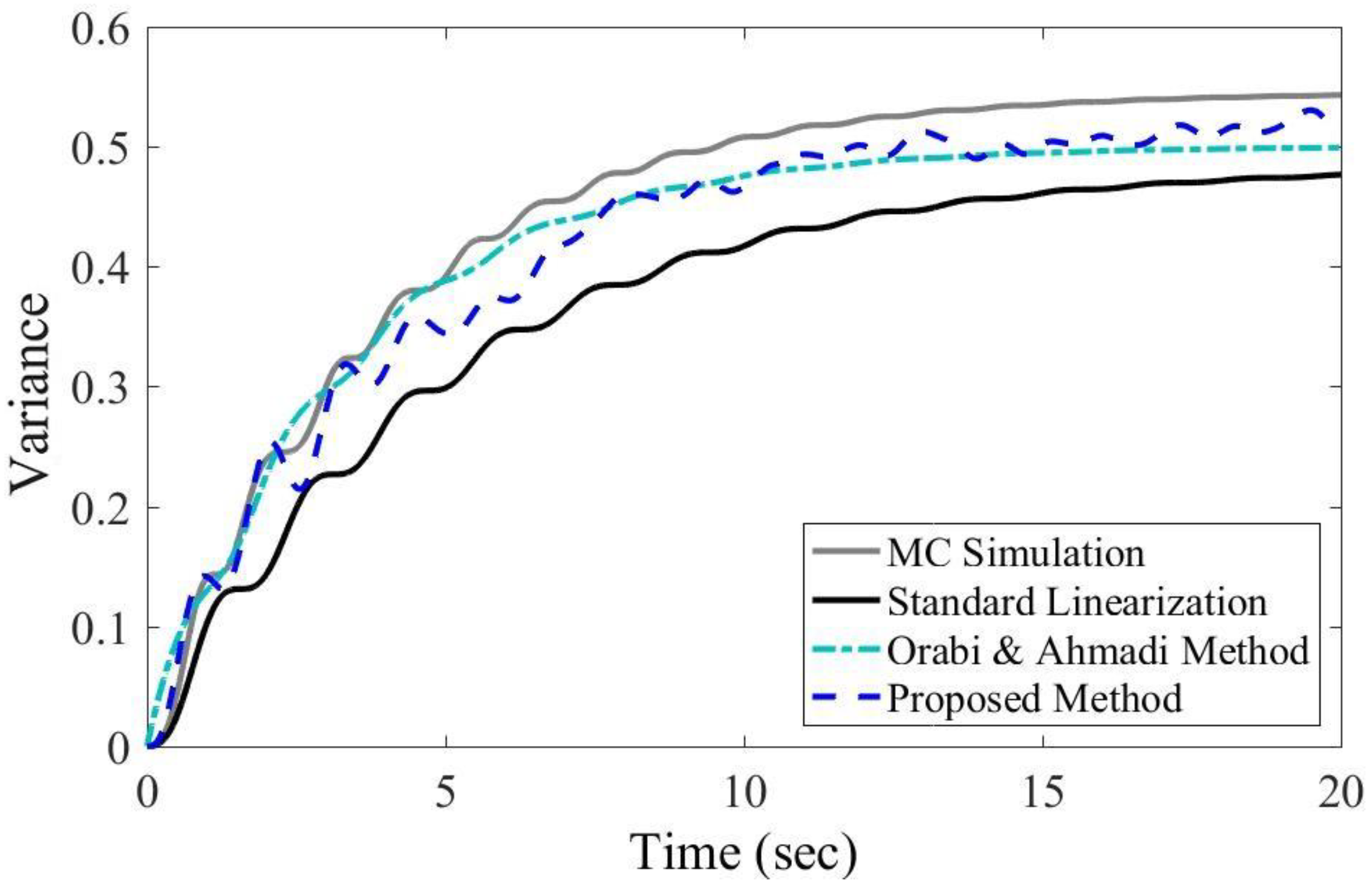
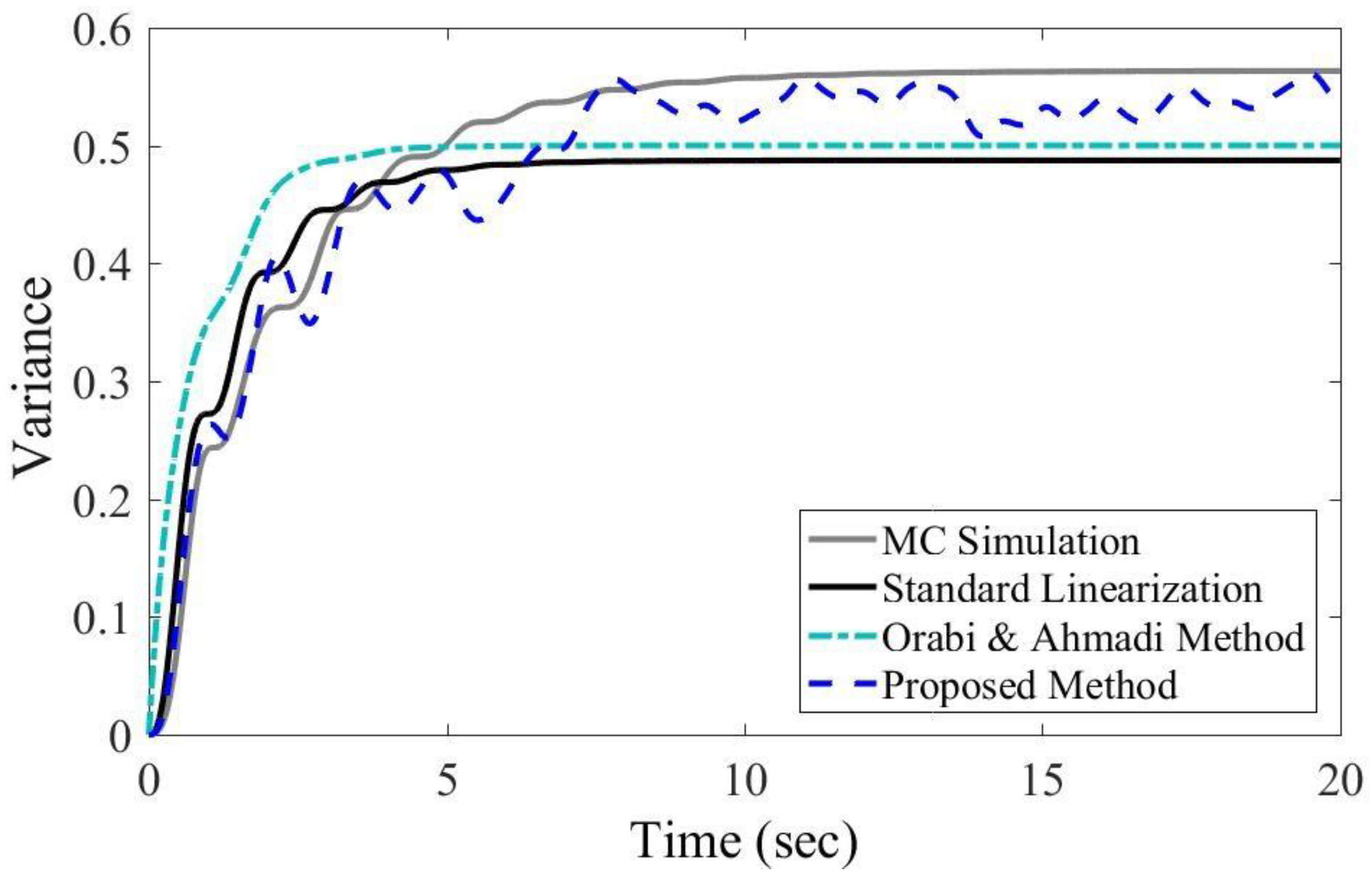
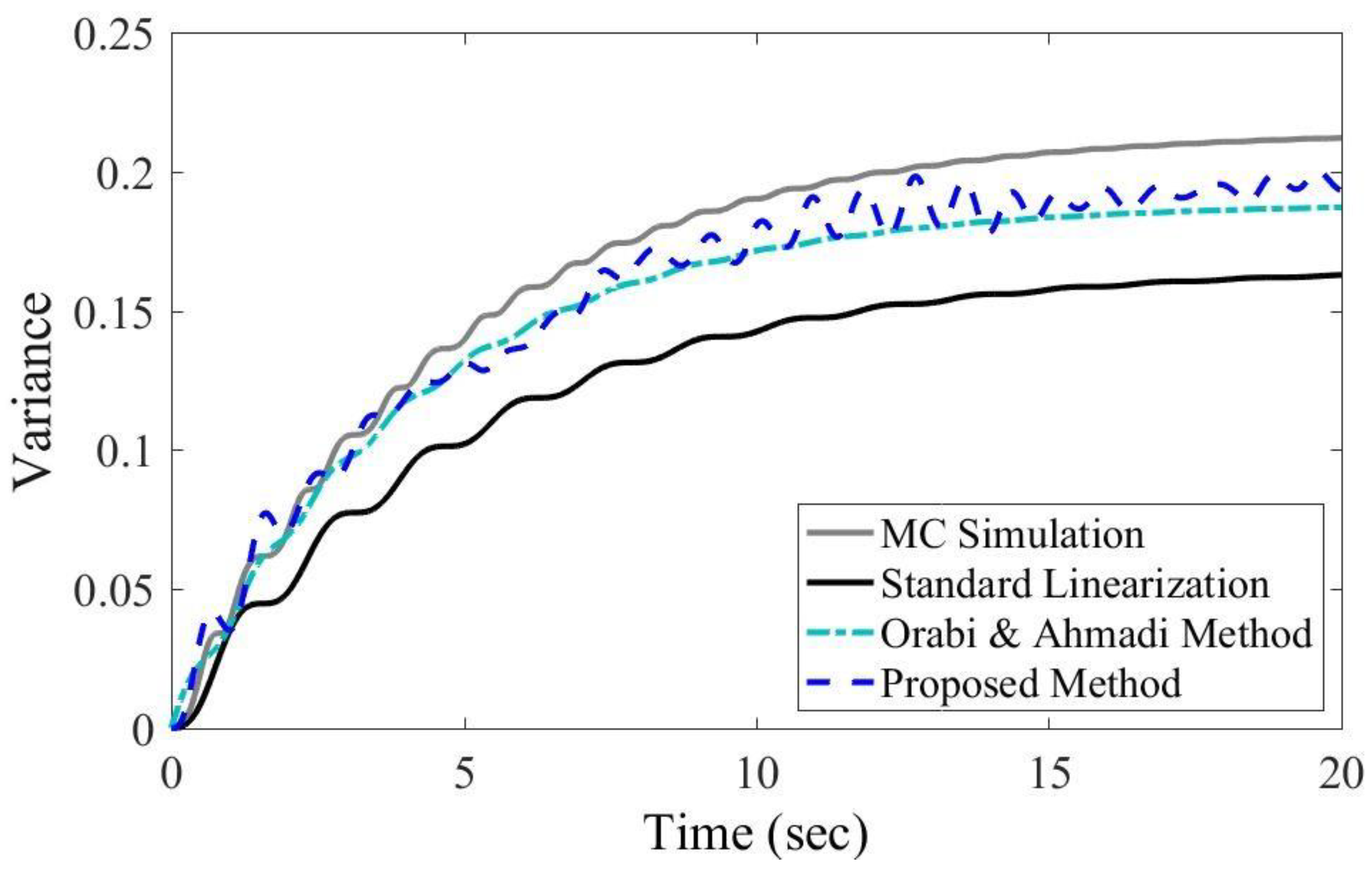
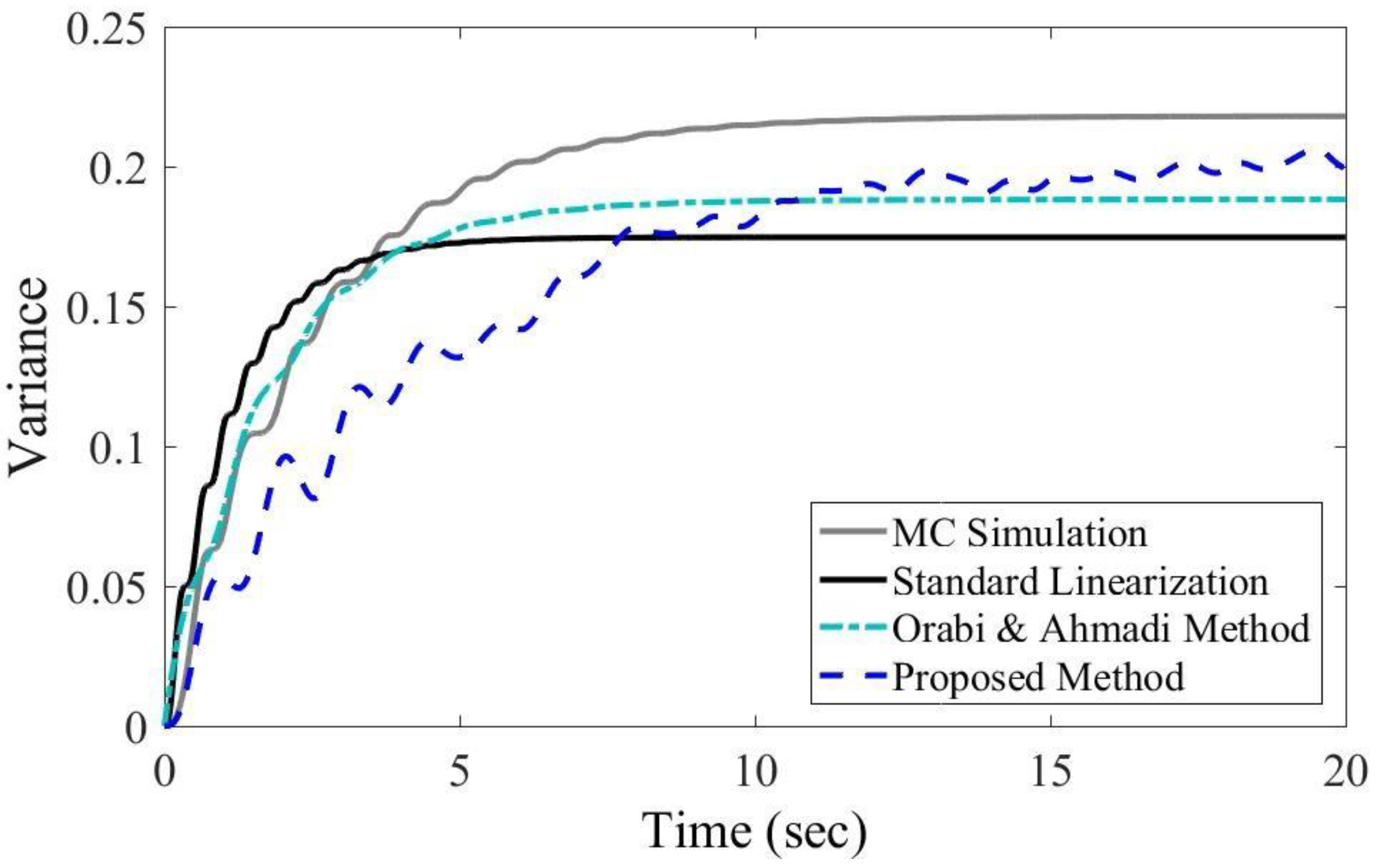
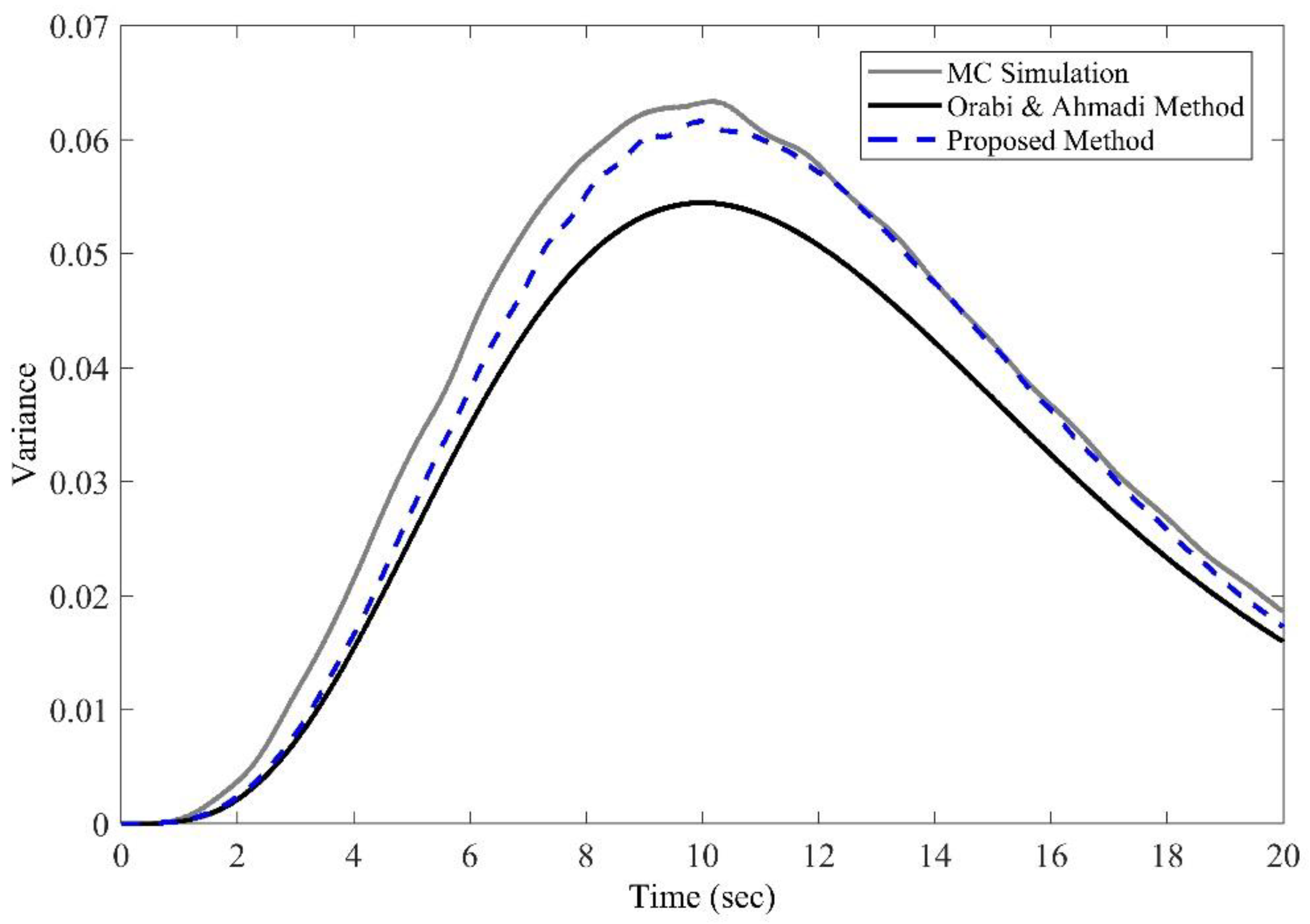
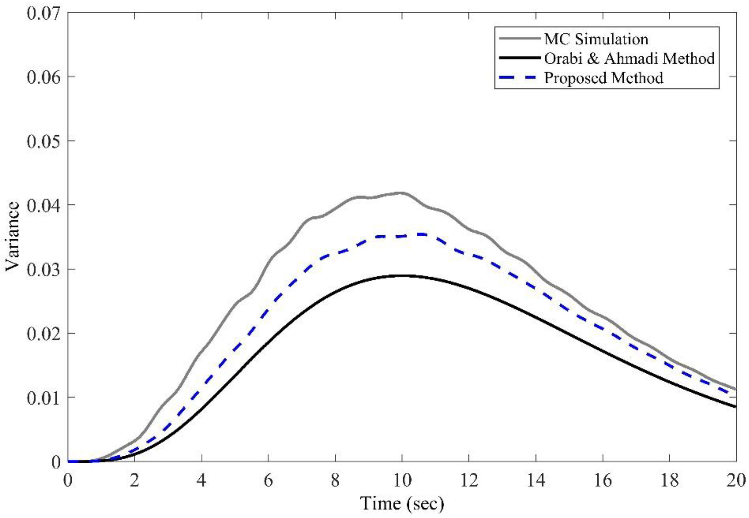
4.1.2. Nonstationary Excitation

Two types of nonstationary excitation are considered for the same SDOF Duffing–Van der Pol oscillator, i.e., a nonwhite noise function and the El Centro (1940) earthquake record.

(a)

Nonwhite noise forcing function

This forcing function can be expressed as

$$f\left(t\right)=\sum _{j=1}^{m}t{a}_{j}exp\left\{-{\beta }_{j}t\right\}\mathrm{c}\mathrm{o}\mathrm{s}({\omega }_{j}t+\theta )$$

(42)

where $a_j$, ${\beta }_j$, ${\omega }_j$ are constant system parameters, and $\theta$ is a random variable uniformly distributed over $[0,2\pi ]$. The forcing function in Equation (42) was proposed by Bogdanoff et al. [30] as a model to describe the ground acceleration induced by earthquake. Again, by using the proposed method, Equation (38) can be solved and the response variance due to this nonstationary excitation can be computed at each time step. If ${\rho }_1=0.$2 and ${\omega }_1=1$ were assumed, the system parameters in Equation (42) would become

$$a_j=1,\hspace{1em}{\omega }_j=j{\omega }_1,\hspace{1em}{\beta }_j={\rho }_1{\omega }_j$$

(43)

Under this set of system parameters, the mean square response of the Duffing–Van der Pol oscillator was evaluated for two different nonlinearity strengths of $\gamma =\mu =1.0$ and $\gamma =\mu =10.0$. The results are shown in Figure 6, Figure 7, Figure 8 and Figure 9. For the convenience of comparison, the results predicted by the iteration method in [10] and the MC simulation are also shown in these four figures.

Similarly, results in Figure 6, Figure 7, Figure 8 and Figure 9 indicate clearly that the proposed orthogonal-function-based equivalent linearization method can give more accurate predictions on system response than the existing approach. As the system behavior becomes less nonlinear, the responses predicted by the proposed method become more agreeable with that of the MC simulation. These suggest that the proposed approach is equally applicable to an SDOF nonlinear system subjected to both stationary and nonstationary excitations. Meanwhile, it can be seen that a stronger nonlinearity in the system stiffness could have a more considerable impact on the accuracy of the existing methods.

A comparison has been carried out between the proposed method and the method by Orabi and Ahmadi [10] in terms of the number of iterations required for convergence to evaluate the computational efficiency. The results are shown in

Table 2. Comparison of the number of iterations.

	Strength of Nonlinearity
	γ = 1.0, μ = 1.0	γ = 1.0, μ = 10	γ =10, μ = 1.0	γ = 10, μ = 10
Orabi and Ahmadi Method [10]	7	8	11	17
Present Method	4	6	8	10

.

It can be seen that for the four studied levels of nonlinearity strength, the proposed method requires fewer iterations than the existing method in [10].

(b)

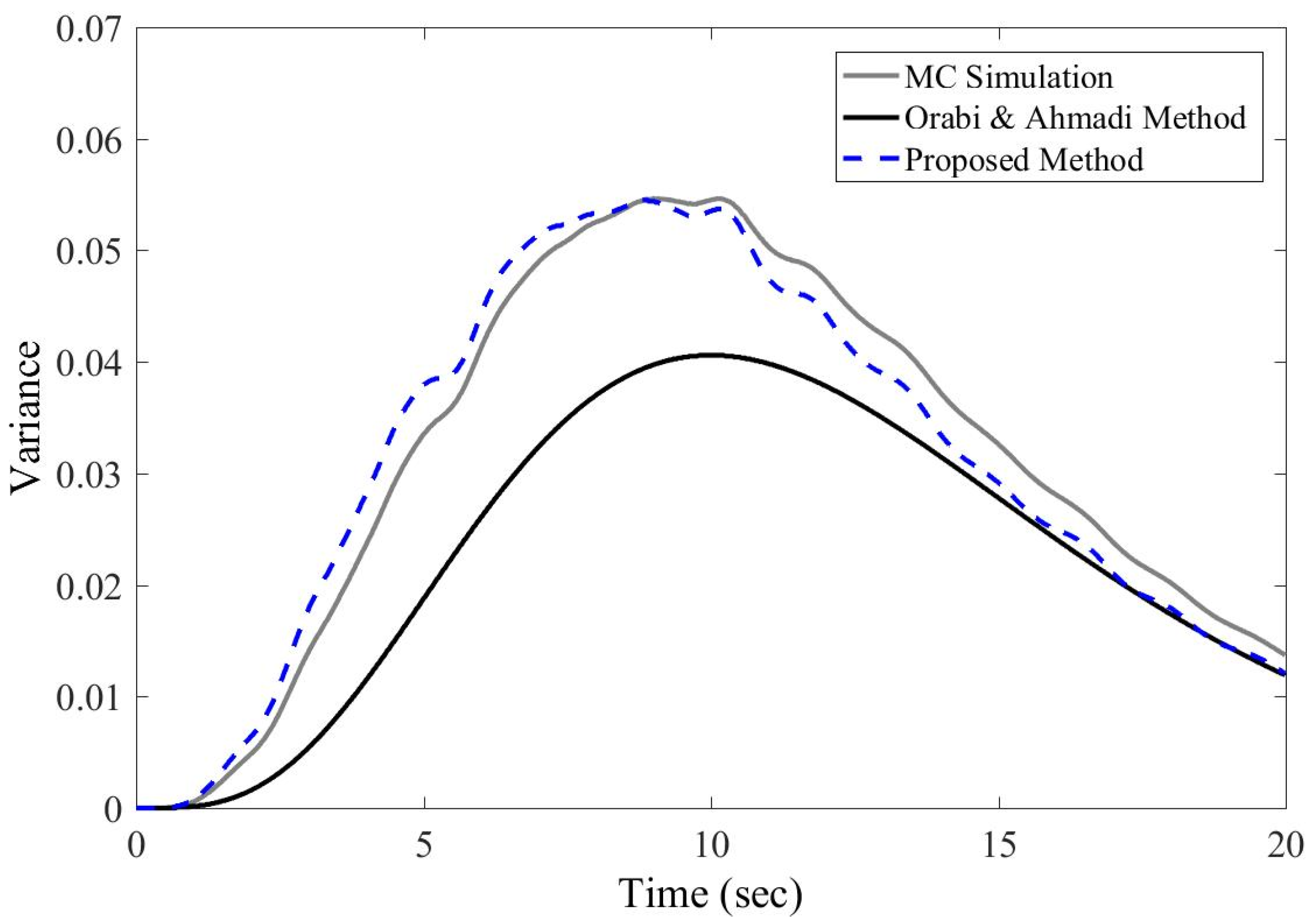
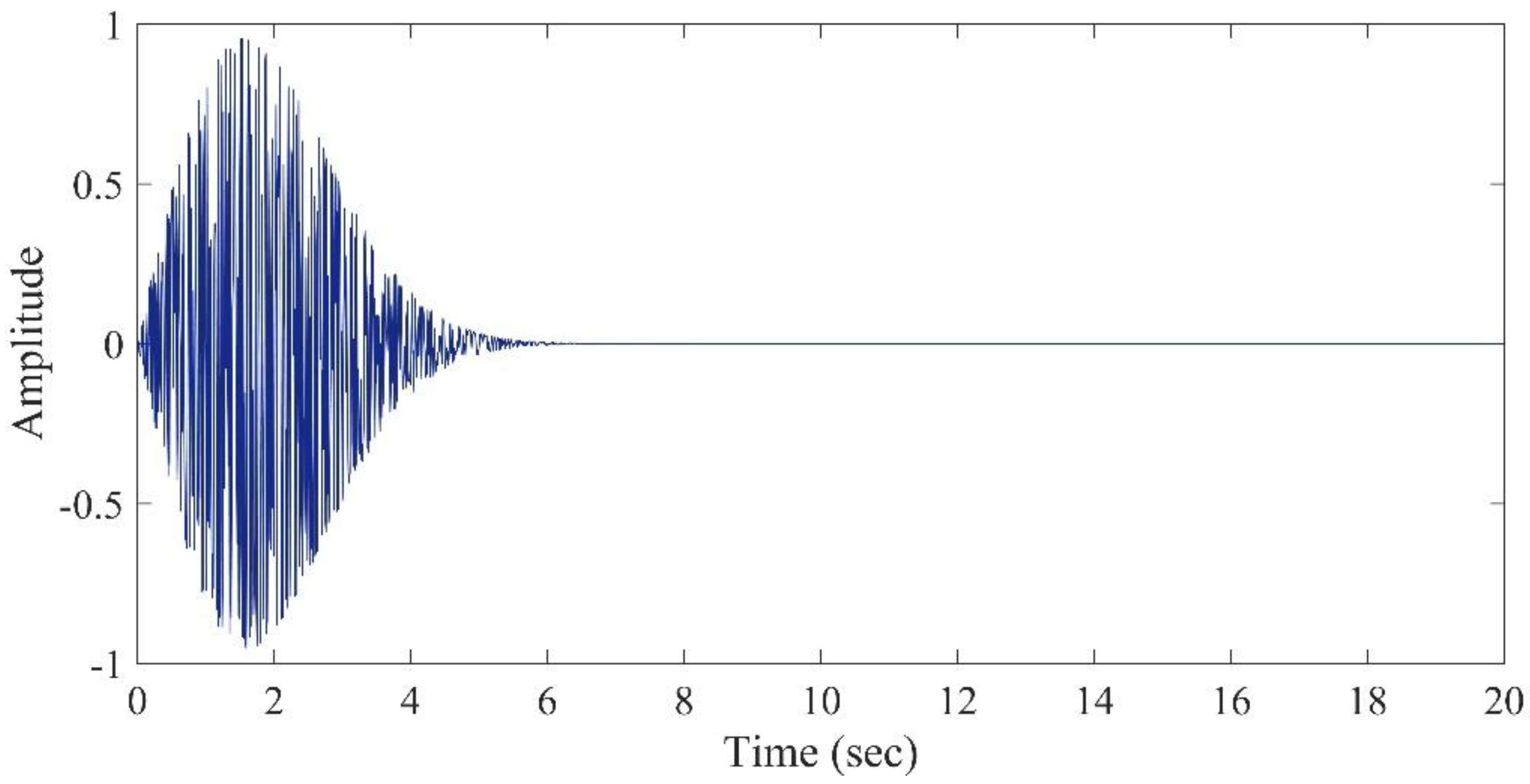
El Centro (1940) earthquake record with $S_0=55.44$

Figure 10 illustrates the mean square displacement response of the studied SDOF nonlinear Duffing–Van der Pol oscillator when subjected to a nonstationary excitation in terms of the El Centro (1940) earthquake record with $S_0=55.44$ at three different levels of stiffness nonlinearity strength of $\gamma =0.0$ (linear), 5.0 and 15.0, when the nonlinearity strength of damping remains at $\mu =1.0$. In addition, Figure 11 shows the mean square displacement response of the considered oscillator at three different damping nonlinearity strength levels of $\mu =0.0$ (linear), 5.0 and 15.0, when the stiffness nonlinearity strength is $\gamma =1.0$.

From Figure 10 and Figure 11, it is obvious that the mean square displacement time histories of all three nonlinearity strength scenarios manifest the same pattern. The responses reach the peak value at about 4 to 6 s and then decrease gradually. In addition, it is observed that the damping nonlinearity has less impact on $E\left[x^2\right]$ values in comparison with stiffness nonlinearity. As expected, the linear system ($\gamma =\mu =0$) has the largest variance and the response amplitude decreases as the strength of nonlinearity increases.

This example demonstrates that the proposed method is applicable to analyze the response of a nonlinear SDOF system subjected to either stationary or nonstationary excitations with high accuracy. The introduction of orthogonal functions can considerably reduce computational effort in the linearization procedures. The proposed method will be extended to a 5DOF nonlinear Duffing–Van der Pol oscillator in the next section to evaluate its applicability to an MDOF nonlinear system subjected to nonstationary excitations.

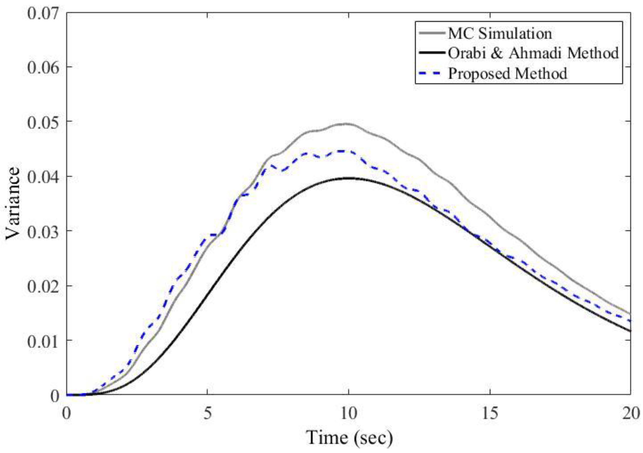
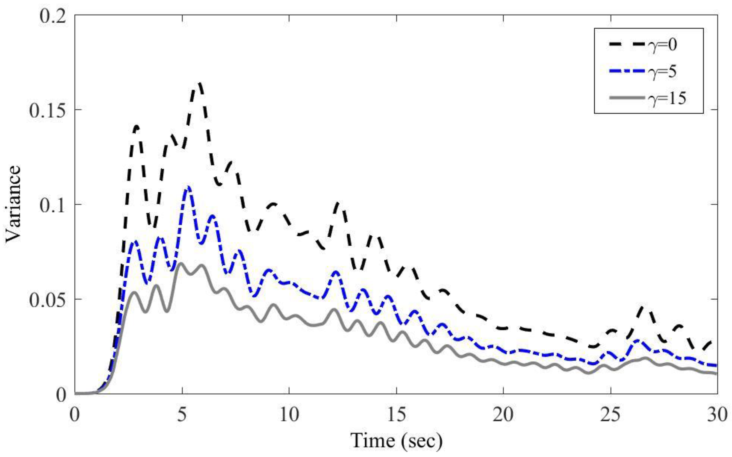
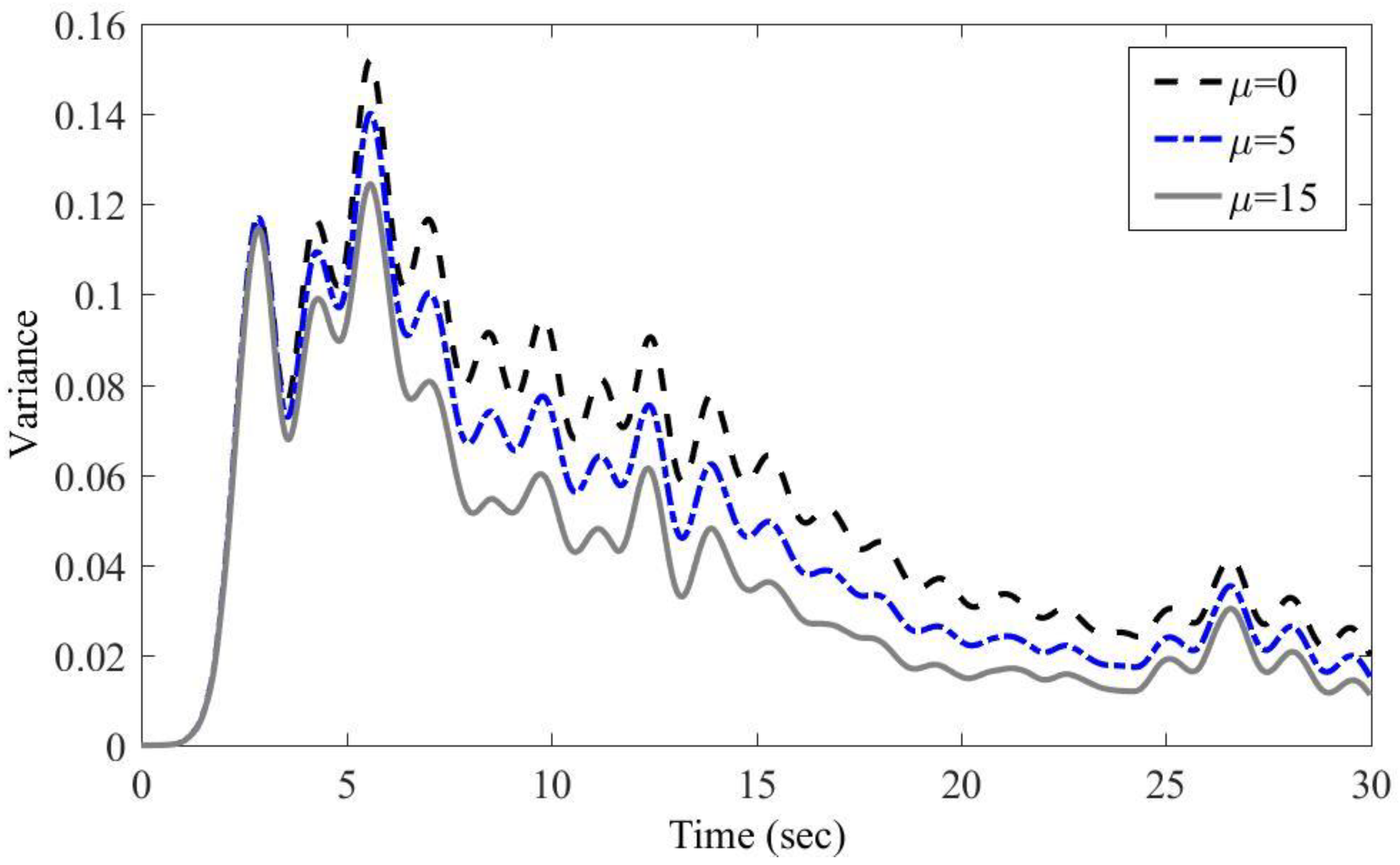
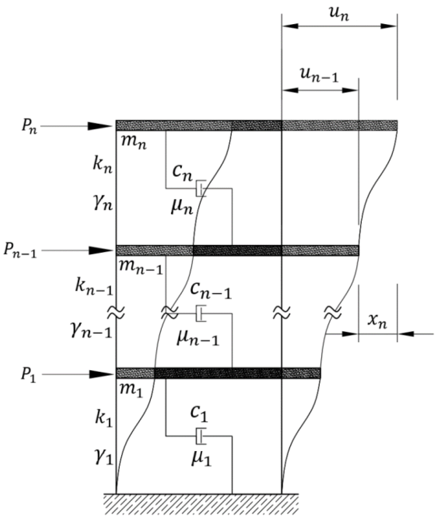
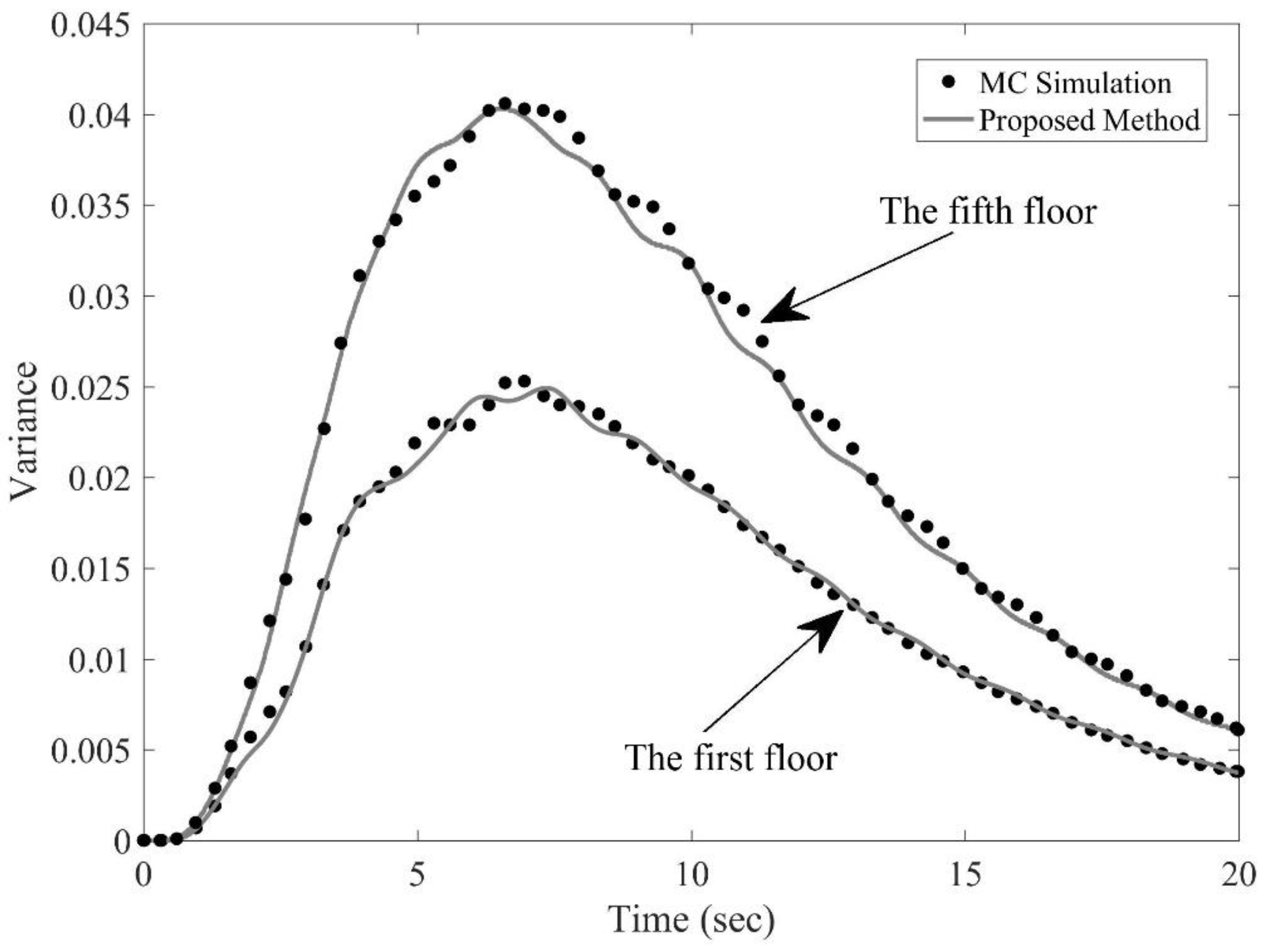
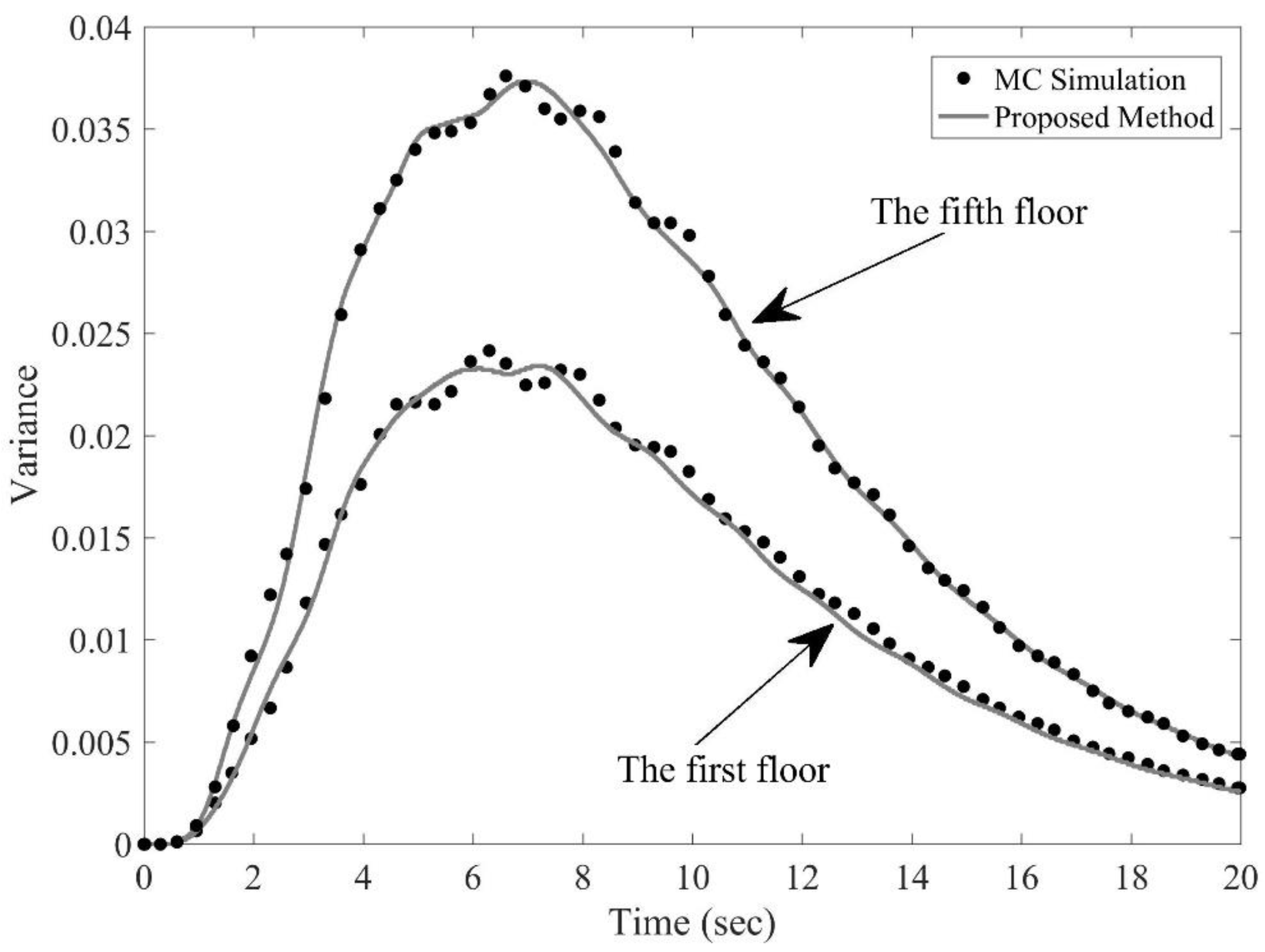
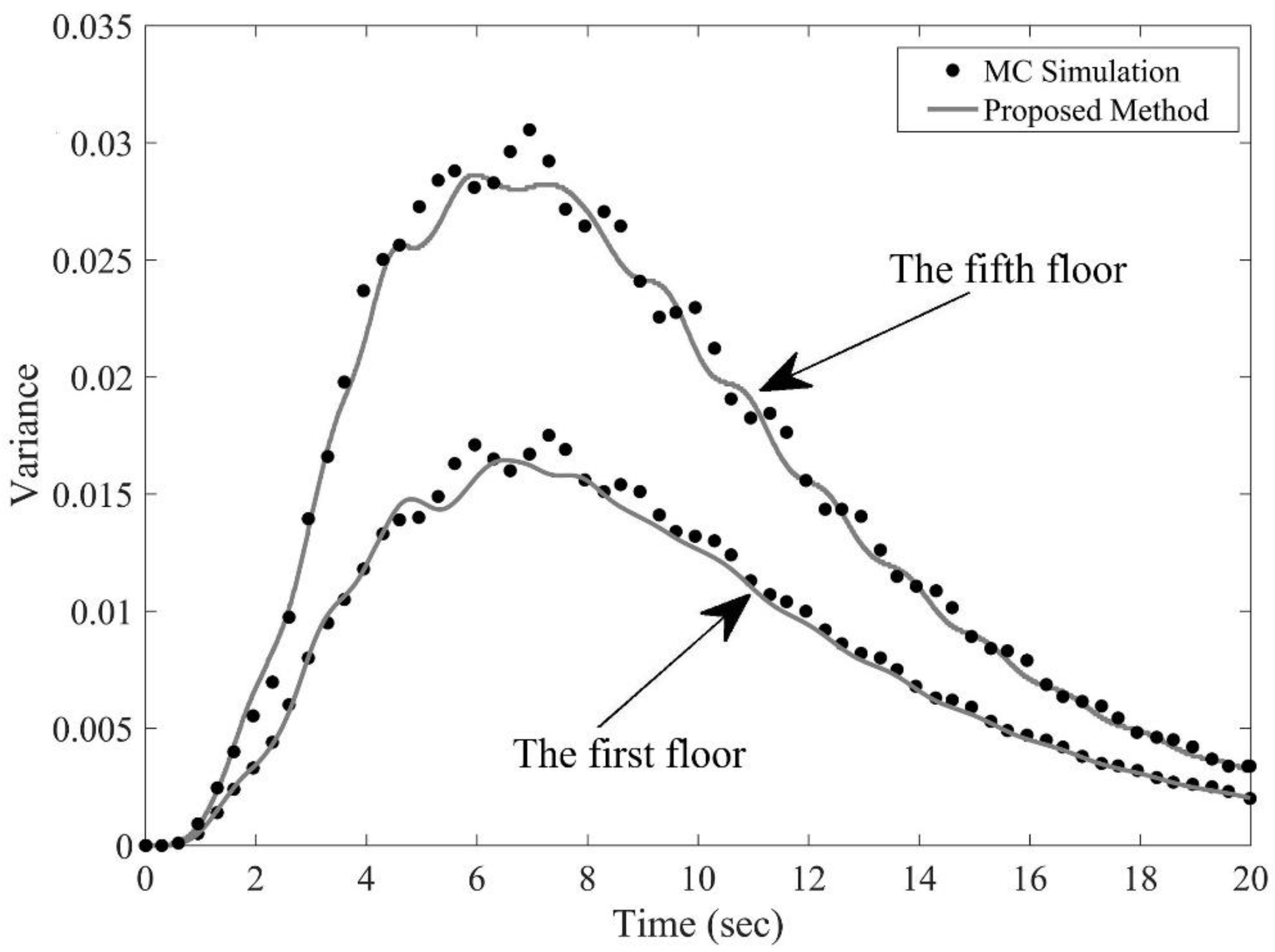
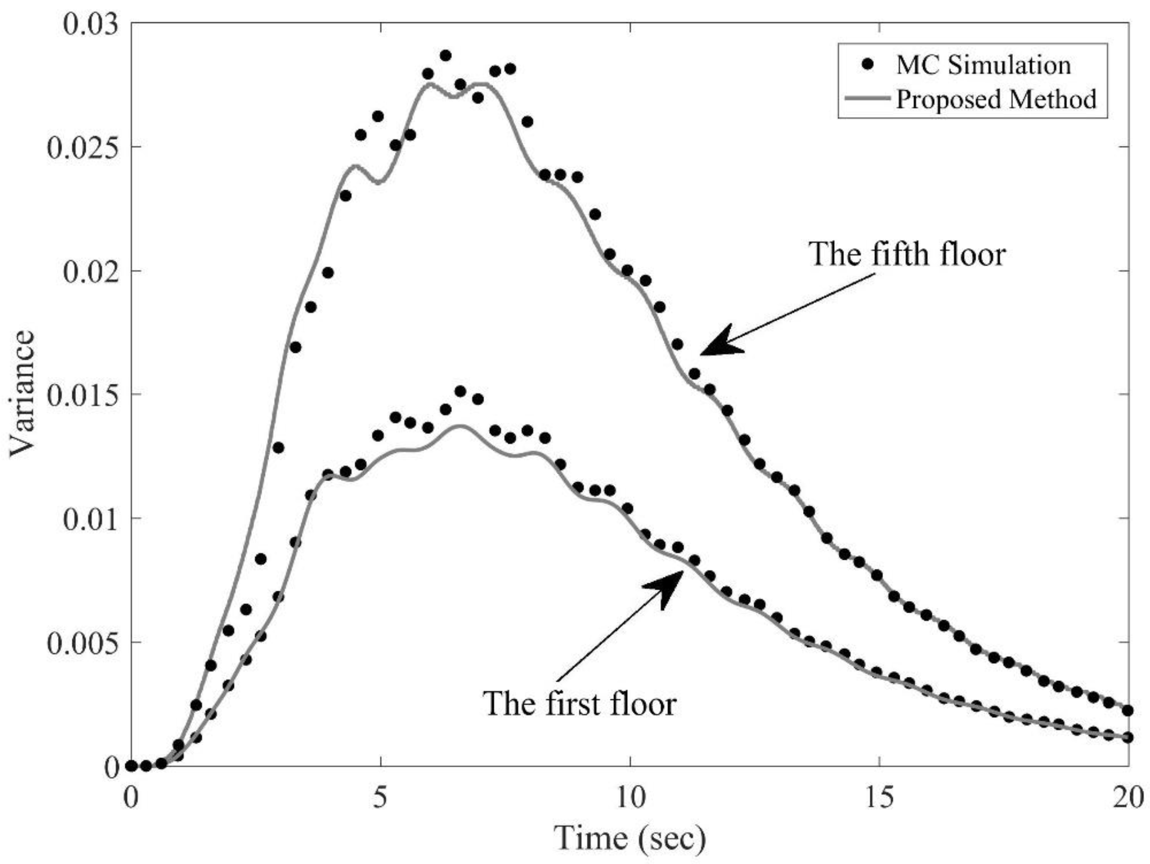
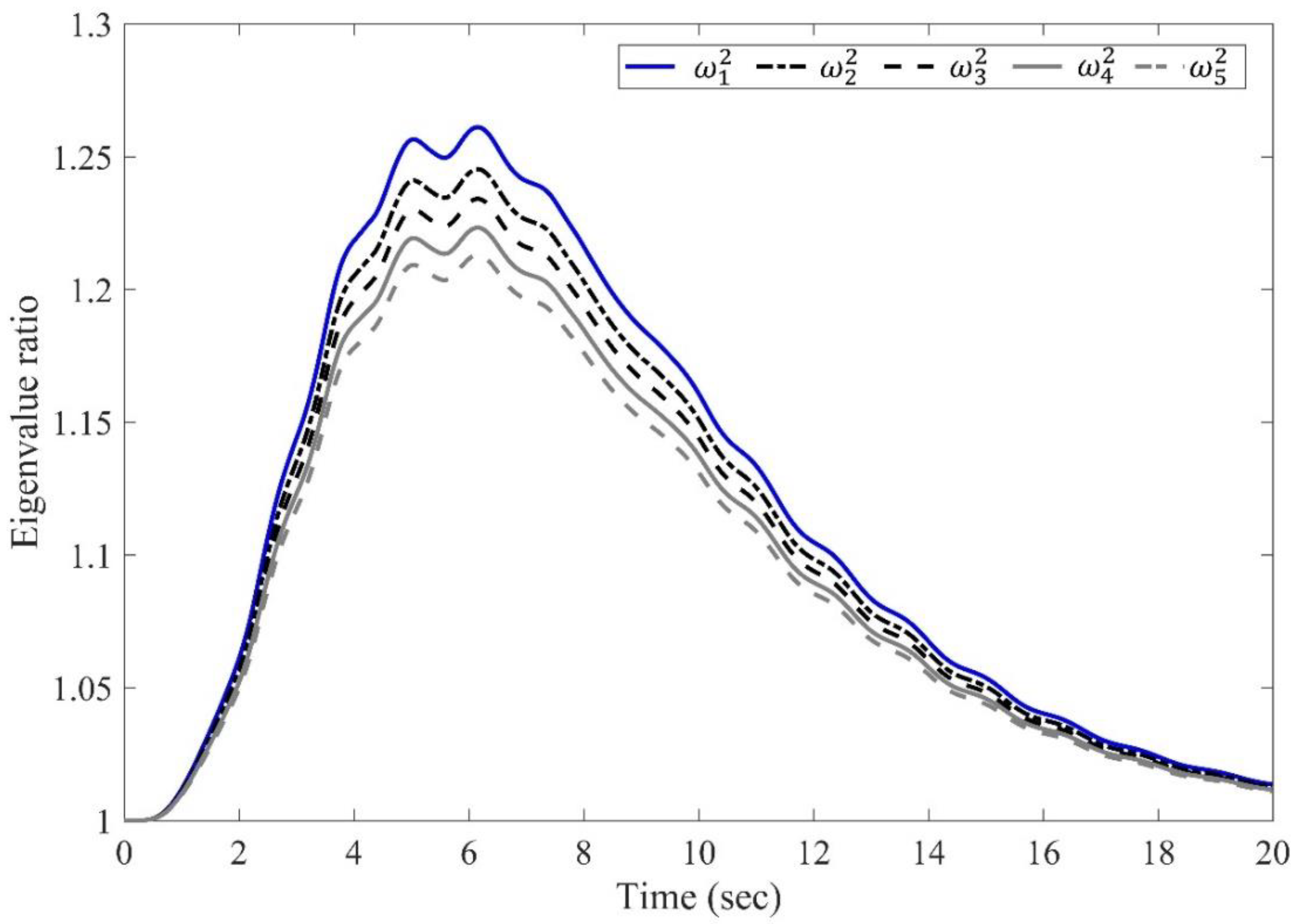
4.2. MDOF Duffing–Van der Pol Oscillator

The equation of motion of the n-degree-of-freedom Duffing–Van der Pol system shown in Figure 12 is shown in Equation (44).

$$\mathit{M}\ddot{\mathit{U}}\left(t\right)+\mathit{C}\dot{\mathit{U}}\left(t\right)+\mathit{K}\mathit{U}\left(t\right)+\mathit{L}\left(\mathit{t}\right)+\mathit{G}\left(t\right)=\mathit{P}(t)$$

(44)

where $\mathit{U}\left(t\right),\dot{\mathit{U}}\left(t\right)$ and $\ddot{\mathit{U}}(t)$ denote the horizontal displacement vector, the corresponding velocity vector and the acceleration vector, respectively, i.e.,

$$\ddot{\mathit{U}}\left(t\right)=\left[\begin{array}{c}{\ddot{u}}_1\\ {\ddot{u}}_2\\ \begin{array}{c}⋮\\ {\ddot{u}}_n\end{array}\end{array}\right]; \dot{\mathit{U}}\left(t\right)=\left[\begin{array}{c}{\dot{u}}_1\\ {\dot{u}}_2\\ \begin{array}{c}⋮\\ {\dot{u}}_n\end{array}\end{array}\right]; \mathit{U}\left(t\right)=\left[\begin{array}{c}{u}_1\\ u_2\\ \begin{array}{c}⋮\\ u_n\end{array}\end{array}\right]$$

(45)

where ${\ddot{u}}_i$, ${\dot{u}}_i$ and $u_i$ $(i=1,2,\dots ,n)$ are, respectively, the horizontal acceleration, velocity and displacement of the i-th floor. $\mathit{P}\left(t\right)=\mathit{\varphi }\mathit{W}\left(t\right)$, where $\mathit{\varphi }$ is the orientation matrix of the nonstationary zero-mean Gaussian random excitation $\mathit{W}\left(t\right)$ and the nonlinear terms $\mathit{G}\left(t\right)$ and $\mathit{L}\left(t\right)$ can be expressed as

$$\mathit{G}\left(t\right)=\left[\begin{array}{c}{\gamma }_1{k}_1{x}_1^3-{\gamma }_2{k}_2{x}_2^3\\ \begin{array}{c}{\gamma }_2{k}_2{x}_2^3-{\gamma }_3{k}_3{x}_3^3\\ {\gamma }_3{k}_3{x}_3^3-{\gamma }_4{k}_4{x}_4^3\end{array}\\ \begin{array}{c}⋮\\ {\gamma }_{n-1}{k}_{n-1}{x}_{n-1}^3-{\gamma }_n{k}_n{x}_n^3\\ {\gamma }_n{k}_n{x}_n^3\end{array}\end{array}\right];\left[\begin{array}{c}{x}_1\\ \begin{array}{c}{x}_2\\ x_3\end{array}\\ \begin{array}{c}⋮\\ x_{n-1}\\ x_n\end{array}\end{array}\right]=\left[\begin{array}{c}{u}_1\\ \begin{array}{c}{u}_2-u_1\\ u_3-u_2\end{array}\\ \begin{array}{c}⋮\\ u_{n-1}-u_{n-2}\\ u_n-u_{n-1}\end{array}\end{array}\right]$$

(46)

$$\mathit{L}\left(t\right)=\left[\begin{array}{c}{\mu }_1{c}_1{x}_1^2{\dot{x}}_1-{\mu }_2{c}_2{x}_2^2{\dot{x}}_2\\ \begin{array}{c}{\mu }_2{c}_2{x}_2^2{\dot{x}}_2-{\mu }_3{c}_3{x}_3^2{\dot{x}}_3\\ {\mu }_3{c}_3{x}_3^2{\dot{x}}_3-{\mu }_4{c}_4{x}_4^2{\dot{x}}_4\end{array}\\ \begin{array}{c}⋮\\ {\mu }_{n-1}{c}_{n-1}{x}_{n-1}^2{\dot{x}}_{n-1}-{\mu }_n{c}_n{x}_n^2{\dot{x}}_n\\ {\mu }_n{c}_n{x}_n^2{\dot{x}}_n\end{array}\end{array}\right];\left[\begin{array}{c}{\dot{x}}_1\\ \begin{array}{c}{\dot{x}}_2\\ {\dot{x}}_3\end{array}\\ \begin{array}{c}⋮\\ {\dot{x}}_{n-1}\\ {\dot{x}}_n\end{array}\end{array}\right]=\left[\begin{array}{c}{\dot{u}}_1\\ \begin{array}{c}{\dot{u}}_2-{\dot{u}}_1\\ {\dot{u}}_3-{\dot{u}}_2\end{array}\\ \begin{array}{c}⋮\\ {\dot{u}}_{n-1}-{\dot{u}}_{n-2}\\ {\dot{u}}_n-{\dot{u}}_{n-1}\end{array}\end{array}\right]$$

(47)

where $x_i$ and ${\dot{x}}_i$ are the relative displacement and velocity between the i-th and (i − 1)-th floors and can be expressed as $x_i=u_i-u_{i-1}$ and ${\dot{x}}_i={\dot{u}}_i-{\dot{u}}_{i-1}(i=\mathrm{1,2},\dots ,n)$ with $u_0={\dot{u}}_0=0$; $k_i$ and $c_i$ $(i=\mathrm{1,2},\dots ,n)$ are the linear stiffness and damping coefficients of the i-th story and ${\gamma }_i$ and ${\mu }_i$ $(i=\mathrm{1,2},\dots ,n)$ are the coefficients reflecting the stiffness and damping nonlinearity at the i-th story.

Substituting Equations (46) and (47) into Equations (17) and (18), the equivalent linearized damping and stiffness matrices for Equation (30) can be obtained at the relevant time instant $\tau$ as

$${\mathit{C}}_{\mathit{e}\mathit{q}}\left(\tau \right)=\left[\begin{array}{cccccc}{{\rm Y}}_1\left(\tau \right)+{{\rm Y}}_2\left(\tau \right)& {-{\rm Y}}_2\left(\tau \right)& & 0& \dots & 0\\ {-{\rm Y}}_2\left(\tau \right)& {{\rm Y}}_2\left(\tau \right)+{{\rm Y}}_3\left(\tau \right)& & {-{\rm Y}}_3\left(\tau \right)& & \\ 0& {-{\rm Y}}_3\left(\tau \right)& & & & ⋮\\ ⋮& & & \ddots & & {-{\rm Y}}_n\left(\tau \right)\\ 0& \dots & & {-{\rm Y}}_n\left(\tau \right)& & {{\rm Y}}_n\left(\tau \right)\end{array}\right]$$

(48)

$${\mathit{K}}_{\mathit{e}\mathit{q}}\left(\tau \right)=3\left[\begin{array}{cccccc}{\chi }_1\left(\tau \right)+{\chi }_2\left(\tau \right)& {-\chi }_2\left(\tau \right)& & 0& \dots & 0\\ {-\chi }_2\left(\tau \right)& {\chi }_2\left(\tau \right)+{\chi }_3\left(\tau \right)& & {-\chi }_3\left(\tau \right)& & \\ 0& {-\chi }_3\left(\tau \right)& & & & ⋮\\ ⋮& & & \ddots & & {-\chi }_n\left(\tau \right)\\ 0& \dots & & {-\chi }_n\left(\tau \right)& & {\chi }_n\left(\tau \right)\end{array}\right]$$

(49)

where

$${{\rm Y}}_i\left(\tau \right)={\mu }_i{c}_{i}E\left[x_i^2\left(\tau \right)\right]={\mu }_i{c}_i\left(E\left[u_i^2\left(\tau \right)\right]-E\left[u_i\left(\tau \right)u_{i-1}\left(\tau \right)\right]+E\left[u_{i-1}^2\left(\tau \right)\right]\right)$$

(50)

$${\chi }_i\left(\tau \right)={\gamma }_i{k}_{i}E\left[x_i^2\left(\tau \right)\right]={\gamma }_i{k}_i\left(E\left[u_i^2\left(\tau \right)\right]-E\left[u_i\left(\tau \right)u_{i-1}\left(\tau \right)\right]+E\left[u_{i-1}^2\left(\tau \right)\right]\right)$$

(51)

Accordingly, the time-invariant equivalent linear system for the studied MDOF Duffing system at time instant $\tau$ can be described using the following equivalent linear equation of motion as

$$\mathit{M}\ddot{\mathit{U}}\left(t\right)+[\mathit{C}+{\mathit{C}}_{\mathit{e}\mathit{q}}(\tau \left)\right]\dot{\mathit{U}}\left(t\right)+\left[\mathit{K}+{\mathit{K}}_{\mathit{e}\mathit{q}}\left(\tau \right)\right]\mathit{U}\left(t\right)=\mathit{\varphi }\mathit{W}\left(t\right)$$

(52)

where $\mathit{U}\left(t\right)=\left[u_1{u}_2\dots u_n\right]$.

It can be seen from Equations (48)–(51) that, at the relevant time instant $\tau$, the linear equivalent damping and stiffness matrices ${\mathit{C}}_{\mathit{e}\mathit{q}}\left(\tau \right)$ and ${\mathit{K}}_{\mathit{e}\mathit{q}}\left(\tau \right)$ are dependent on the second-order moment of the responses at the same time instant, which, in turn, need to be determined through the nonstationary random vibration analysis of the equivalent linear system based on Equation (52). Therefore, an iterative procedure based on a series of nonstationary linear random vibration analyses at each time instant is required.

As an illustrative example, we now consider a 5DOF Duffing–Van der Pol system. The lumped masses of the system are taken to be $m_{\mathrm{1,2},3}=4 \mathrm{k}\mathrm{g}$ and $m_{\mathrm{4,5}}=3 \mathrm{k}\mathrm{g}$ and the linear stiffnesses of the five stories are assumed to be $k_{\mathrm{1,2},3}=150 \mathrm{N}/\mathrm{m}$ and $k_{\mathrm{4,5}}=100 \mathrm{N}/\mathrm{m}$. The Rayleigh damping model is adopted to define the damping matrix and a critical damping ratio of 0.05 is assumed for the first mode and the 5th mode of the initial linear system. Two nonlinearity cases are considered with the nonlinear strength coefficients being ${\gamma }_i={\mu }_i=1$ and ${\gamma }_i={\mu }_i=10(i=1; 2; \dots , 5)$. The system is subjected to a nonstationary random process defined by Equation (42) for the same excitation parameters chosen for the SDOF Duffing-Van der Pol system except with ${\rho }_1=0.3$, which is shown in Figure 13.

The orthogonal-function-based equivalent linearization method is used to determine the variance of displacements at each floor. Again, to check the accuracy of the proposed method, the MC simulation method with 1000 samples was exploited. Figure 14, Figure 15, Figure 16 and Figure 17 show the mean square lateral displacements of the first and the fifth floor of the studied 5DOF Duffing–Van der Pol system.

It is observed from Figure 14, Figure 15, Figure 16 and Figure 17 that of the four studied nonlinearity strength cases, the responses predicted by the proposed approach are in good agreement with those of the MC simulation, with the maximum relative difference between the two methods for ${\gamma }_i={\mu }_i=1$ and ${\gamma }_i={\mu }_i=10$ being 1.9% and 6.2%, respectively. Furthermore, the results suggest that increasing the strength of stiffness nonlinearity would decrease the accuracy of the proposed method. This not only demonstrates the accuracy of the proposed method, but also indicates that as the nonlinearity of a system becomes stronger, the application of the proposed equivalent linearization method would cause relatively larger error in the predicted response. This fact is understandable, as the accuracy of the equivalent linearization method decreases for strongly nonlinear systems.

In addition, the eigenvalue ratios between the equivalent linear system and the original nonlinear one are shown in Figure 18 for the first five system modes when ${\gamma }_i={\mu }_i=10$. The pattern of the curves in Figure 18 suggests that the presence of nonlinearity has the most impact on the system’s fundamental mode, whereas its influence becomes less for the higher-order modes. It can be seen from the figure that for all five studied modes, the eigenvalue ratios gradually increase until they reach the maximum value at $t=6.11 \mathrm{s}$. In particular, the eigenvalue ratio associated with the system’s fundamental mode increases up to 26.62% at this time instance, indicating a significant increase in nonlinearity in the system response within this time period. However, the magnitude of these five eigenvalue ratios decreases afterward and converges to the same value of 1.013 at $t=20 \mathrm{s},$ which implies that the nonlinearity of the system becomes progressively weaker, and the system eventually behaves almost linearly. This “increase and then decrease” pattern of the system nonlinearity is caused by the form of the nonstationary excitation applied to the system. As shown in Figure 13, the amplitude of the given nonstationary excitation increases monotonically within the first 1.5 s, then gradually decreases and diminishes slightly after 6 s. Thus, within the first 6 s or so, the system is under forced vibration. The input energy by the excitation is more than that dissipated by system damping. Therefore, the response amplitude gradually builds up, and the nonlinearity becomes stronger, whereas beyond that, the system is under free vibration, of which the accumulated energy is gradually dissipated by the damping mechanism. Thus, the response amplitude becomes less and less, which weakens the system nonlinearity strength until it behaves more like a linear system.

Table 3. Comparison of the required time by the MC simulation method and the proposed method.

	Strength of Nonlinearity
	γ = 1.0, μ = 1.0	γ = 1.0, μ = 10	γ = 10, μ = 1.0	γ = 10, μ = 10
$\mathrm{MC}\mathrm{Simulation}\mathrm{Method}{(T}_1)$	3120 s	3201 s	3580 s	3666 s
$\mathrm{Proposed}\mathrm{Method}{(T}_2)$	26.25 s	47.5 s	48.1 s	67 s
$T_1/T_2$	119	67	74	55

lists the computation time required by the MC simulation method and the proposed method for different studied scenarios. Results show that the total computation time needed by the MC simulation method is significantly longer than that by the proposed method in all cases. The comparison indicates that the proposed method has a very high computational efficiency for nonlinear systems. It should be mentioned that all computations were performed on a computer with Intel Core i7 2600, 2.0 GHz processor and 4 G of RAM.

5. Conclusions

This study suggests a time domain method for applying orthogonal functions to accurately approximate the responses of nonlinear systems to nonstationary excitations. The formulation of the proposed method has been presented first, and its validity and accuracy have been verified through numerical examples. An SDOF nonlinear Duffing–Van der Pol oscillator subjected to stationary or nonstationary excitation is taken into consideration for this purpose. Then, the methodology is extended to analyzing a 5DOF nonlinear Duffing–Van der Pol system subjected to nonstationary excitation. Both the existing and suggested methods are used to calculate the mean square system responses related to various nonlinearity levels. Following is a summary of the key findings:

• Compared to other existing equivalent linearization methods, the system responses predicted by the proposed method are in better agreement with those yielded from the MC simulation, which is used as benchmark in this study.
• The proposed method has high computational efficiency compared to MC simulation.
• The proposed method is applicable to any general type of nonstationary random excitations, especially when dealing with systems having higher nonlinearity and more degrees of freedom.

References

- Crandall, S.H. Perturbation Techniques for Random Vibration of Nonlinear Systems. J. Acoust. Soc. Am. 1963, 35, 1700–1705. [Google Scholar] [CrossRef]
- Zhu, W.Q. Nonlinear Stochastic Dynamics and Control in Hamiltonian Formulation. Appl. Mech. Rev. 2006, 59, 230. [Google Scholar] [CrossRef]
- Crandall, S.H. Non-Gaussian Closure for Random Vibration of Non-Linear Oscillators. Int. J. Non. Linear. Mech. 1980, 15, 303–313. [Google Scholar] [CrossRef]
- Caughey, T.K. Response of Van Der Pol’s Oscillator to Random Excitation. J. Appl. Mech. 1959, 26, 345–348. [Google Scholar] [CrossRef]
- Proppe, C.; Pradlwarter, H.; Engineering, G.S.-P. Equivalent Linearization and Monte Carlo Simulation in Stochastic Dynamics. Probabilistic Eng. Mech. 2003, 18, 1–15. [Google Scholar] [CrossRef]
- Bernard, P.; Taazount, M. Random Dynamics of Structures with Gaps: Simulation and Spectral Linearization. Nonlinear Dyn. 1994, 5, 313–335. [Google Scholar] [CrossRef]
- Socha, L. Probability Density Equivalent Linearization Technique for Nonlinear Oscillator with Stochastic Excitations. ZAMM-J. Appl. Math. Mech. Z. Für Angew. Math. Und Mech. 1998, 78, 1087–1088. [Google Scholar] [CrossRef]
- Zhang, R. Work/Energy-Based Stochastic Equivalent Lineariztion with Optimized Power. J. Sound Vib. 2000, 230, 468–475. [Google Scholar] [CrossRef]
- Huang, C.-T.; Iwan, W.D. Equivalent Linearization for the Nonstationary Response Analysis of Nonlinear Systems with Random Parameters. J. Eng. Mech. 2006, 132, 465–474. [Google Scholar] [CrossRef]
- Orabi, I.I.; Ahmadi, G. An Iterative Method for Non-Stationary Response Analysis of Non-Linear Random Systems. J. Sound Vib. 1987, 119, 145–157. [Google Scholar] [CrossRef]
- Raoufi, R.; Ghafory-Ashtiany, M. Nonlinear Random Vibration Using Updated Tail Equivalent Linearization Method. Int. J. Adv. Struct. Eng. 2014, 6, 1–12. [Google Scholar] [CrossRef] [Green Version]
- Ma, C.; Zhang, Y.; Zhao, Y.; Tan, P.; Zhou, F. Stochastic Seismic Response Analysis of Base-Isolated High-Rise Buildings. Procedia Eng. 2011, 14, 2468–2474. [Google Scholar] [CrossRef] [Green Version]
- Kerschen, G.; Worden, K.; Vakakis, A.F.; Golinval, J.-C. Past, Present and Future of Nonlinear System Identification in Structural Dynamics. Mech. Syst. Signal Process. 2006, 20, 505–592. [Google Scholar] [CrossRef] [Green Version]
- Su, C.; Xu, R. Random Vibration Analysis of Structures by a Time-Domain Explicit Formulation Method. Struct. Eng. Mech. 2014, 52, 239–260. [Google Scholar] [CrossRef]
- Hu, Z.; Su, C.; Chen, T.; Ma, H. An Explicit Time-Domain Approach for Sensitivity Analysis of Non-Stationary Random Vibration Problems. J. Sound Vib. 2016, 382, 122–139. [Google Scholar] [CrossRef]
- Su, C.; Huang, H.; Ma, H. Fast Equivalent Linearization Method for Nonlinear Structures under Nonstationary Random Excitations. J. Eng. Mech. 2016, 142, 04016049. [Google Scholar] [CrossRef]
- Datta, K.B.; Mohan, B.M. Orthogonal Functions in Systems and Control; World Scientific: Singapore, 1995. [Google Scholar]
- Chen, C.F.; Hsiao, C.H. Time-Domain Synthesis via Walsh Functions. Proc. Inst. Electr. Eng. 1975, 122, 565. [Google Scholar] [CrossRef]
- Pacheco, R.P.; Steffen, V. On the Identification of Non-Linear Mechanical Systems Using Orthogonal Functions. Int. J. Non. Linear. Mech. 2004, 39, 1147–1159. [Google Scholar] [CrossRef]
- Younespour, A.; Ghaffarzadeh, H. Structural Active Vibration Control Using Active Mass Damper by Block Pulse Functions. JVC/J. Vib. Control. 2015, 21, 2787–2795. [Google Scholar] [CrossRef]
- Younespour, A.; Ghaffarzadeh, H.; Azar, B.F. An Equivalent Linearization Method for Nonlinear Van Der Pol Oscillator Subjected to Random Vibration Using Orthogonal Functions. Control Theory Technol. 2018, 16, 49–57. [Google Scholar] [CrossRef]
- von Wagner, U.; Wedig, W.V. On the Calculation of Stationary Solutions of Multi-Dimensional Fokker–Planck Equations by Orthogonal Functions. Nonlinear Dyn. 2000, 21, 289–306. [Google Scholar] [CrossRef]
- Aghabalaei Baghaei, K.; Ghaffarzadeh, H.; Younespour, A. Orthogonal Function-based Equivalent Linearization for Sliding Mode Control of Nonlinear Systems. Struct. Control Health Monit. 2019, 26, e2372. [Google Scholar] [CrossRef]
- Younespour, A.; Ghaffarzadeh, H. Semi-Active Control of Seismically Excited Structures with Variable Orifice Damper Using Block Pulse Functions. Smart Struct. Syst. 2016, 18, 1111–1123. [Google Scholar] [CrossRef]
- Jiang, Z.; Schaufelberger, W. Block Pulse Functions and Their Applications in Control Systems; Springer: Berlin/Heidelberg, Germany, 1992. [Google Scholar]
- Atalik, T.S.; Utku, S. Stochastic Linearization of Multi-Degree-of-Freedom Non-Linear Systems. Earthq. Eng. Struct. Dyn. 1976, 4, 411–420. [Google Scholar] [CrossRef]
- Lutes, L.; Sarkani, S. Random Vibrations: Analysis of Structural and Mechanical Systems; Butterworth-Heinemann: Oxford, UK, 2004. [Google Scholar]
- Iwan, W.D.; Yang, I. Application of Statistical Linearization Techniques to Nonlinear Multidegree-of-Freedom Systems. J. Appl. Mech. 1972, 39, 545–550. [Google Scholar] [CrossRef]
- Yamapi, R.; Filatrella, G. Strange Attractors and Synchronization Dynamics of Coupled Van Der Pol–Duffing Oscillators. Commun. Nonlinear Sci. Numer. Simul. 2008, 13, 1121–1130. [Google Scholar] [CrossRef]
- Bogdanoff, J.; Goldberg, J.E.; Bernard, M.C. Response of a Simple Structure to a Random Earthquake-Type Disturbance. Bull. Seismol. Soc. Am. 1961, 51, 293–310. [Google Scholar] [CrossRef]