A Circuit Theory Perspective on the Modeling and Analysis of Vibration Energy Harvesting Systems: A Review

Abstract

This paper reviews advanced modeling and analysis techniques useful in the description, design, and optimization of mechanical energy harvesting systems based on the collection of energy from vibration sources. The added value of the present contribution is to demonstrate the benefits of the exploitation of advanced techniques, most often inherited from other fields of physics and engineering, to improve the performance of such systems. The review is focused on the modeling techniques that apply to the entire energy source/mechanical oscillator/transducer/electrical load chain, describing mechanical–electrical analogies to represent the collective behavior as the cascade of equivalent electrical two-ports, introducing matching networks enhancing the energy transfer to the load, and discussing the main numerical techniques in the frequency and time domains that can be used to analyze linear and nonlinear harvesters, both in the case of deterministic and stochastic excitations.

1. Introduction

The importance of power supply cannot be overstated, especially with reference to Internet of Things (IoT) applications that, nowadays, find their backbone in the deployment of a large number of electronic systems [1]. The current projections assume a growth from the current number of installed IoT devices, estimated to be more than 14 billion, to double this in the second half of the 2020–2030 decade [2]. The very definition of an IoT device is widely general. However, great importance is undoubtedly focused on wireless-connected technologies [3], involving most varied elements (called nodes), such as computers, printers, handheld communication devices, network appliances and smart systems in general. Irrespective of the specific function, each node must be powered, which is a fundamental issue normally tackled by employing wired power supply or batteries. A battery is effective in the case of relatively large and man-handled devices; however, it may become unpractical for miniaturized systems, such as wireless connected sensors (and, in some cases, actuators). In fact, for such nodes the relative size and weight requirements associated to batteries may be too large for the device specifications, not to mention the often difficult physical access, which, in turn, is mandatory in cases of battery maintenance or substitution.

On the other hand, the dispersed nodes can often be designed to require relatively low power, along with a short distance among themselves as a byproduct of their large number. This means that extracting the required energy from the environment may not only be theoretically possible, but also the ideal solution [4]. Energy harvesting refers to a wide range of technological solutions enabling the collection of energy available from the environment and its conversion to electrical form, so as to enable an IoT node power supply either directly or by interposing a buffer battery. Candidate ambient energy sources are quite varied, from mechanical vibrations to electromagnetic radiation, and thermal gradients [5,6,7,8,9].

Ambient mechanical vibrations are a particularly promising source for energy harvesting [5], because they are widespread, they have relatively high power density, and they can be easily converted into usable electrical power exploiting different physical conversion and transduction mechanisms [10].

From the modeling point of view, the mechanical system collecting vibrations can be represented as a forced system characterized by an autonomous oscillating behaviour (namely, by an oscillator), and transferring the harvested mechanical energy to a transduction stage that performs the conversion to the electrical domain.

There are many excellent reviews of energy harvesting technologies and applications, most of them devoted to the harvesting device experimental characterization. Without pretending to be complete. Comprehensive reviews of energy harvesting with piezoelectric materials can be found in [11,12,13,14]. The problem of harvesting kinetic energy at low and high frequencies for wireless applications is reviewed in [8], whereas the problem of broadband energy harvesting is reviewed in [15]. Piezoelectric and electromagnetic technologies for energy harvesting are discussed in [16,17,18]. Excellent reviews on the role of nonlinearity can be found in [19,20,21]. The very important area of applications to implantable medical devices is discussed in [22]. Finally, interesting overviews of solutions to increase the power performance and efficiency of energy harvesters are presented in [23,24].

This paper takes a different perspective. The attention is centered on the harvesting device modeling and methods of analysis, because these aspects provide the foundation for a more systematic approach to the design and optimization of energy harvesting systems. In particular, the focus is on the exploitation of methods from nonlinear dynamics, circuit theory and stochastic analysis to the description of the harvester, which inherently requires a multi-physics representation, as the mechanical and electrical domains, and their interfaces through the energy transduction stage, are all entangled in the device operation. A detailed description of the mechanical part, often carried out through advanced numerical (e.g., finite elements-based) methods [25,26,27] is, thus, avoided. The first part of this contribution reviews the modeling techniques, along with the corresponding challenges, exploited for the description of each stage of the mechanical harvester setup. The second part is devoted to the mathematical methods for the analysis and design of energy harvesters for ambient mechanical vibrations, with particular attention to nonlinear systems. The stochastic techniques enabling the description of the random mechanical vibrations constituting the harvester energy source are discussed in Section 2. The equations of the mechanical system implementing the vibration energy collection (for both the piezoelectric and electromagnetic transducer cases) are presented, and it is shown how an equivalent circuit, representing the entire system dynamics, can be constructed making use of mechanical–electrical analogies. The main advantage of the equivalent circuit description lies in the possible exploitation of well-known load matching techniques, well developed in several electronic circuit areas, to improve, and, in perspective, to maximize, the energy collection efficiency. The final part of Section 2 is devoted to the treatment of nonlinearity in mechanical harvesters, pointing out the major modeling challenges and opportunities. In Section 3 the main analysis approaches, both in the time and in the frequency domains are described. A brief review of frequency domain methods for linear systems is presented, together with an efficient implementation of frequency domain techniques for nonlinear systems, namely the Harmonic Balance technique. The averaging technique for nonlinear systems with periodic or random perturbation is presented next. The last part of Section 3 is dedicated to numerical integration methods, as they represent a fundamental tool for simulation and design, especially in the case of nonlinear systems. Particular attention is given to the intricacies of numerical integration schemes for stochastic differential equations. Finally, Section 4 is devoted to conclusions.

2. Modeling

In this section, the modeling of energy harvesting systems is reviewed. The first problem consists in giving an accurate, yet mathematically tractable, description of mechanical vibrations. The governing equations for two of the most widely used architectures for harvesting vibrational energy, piezoelectric and electromagnetic energy harvesters, are derived. The use of equivalent circuits and the application of load matching solutions to increase the harvested power and power efficiency is presented. Finally, the role of nonlinearities in the governing equation is briefly discussed.

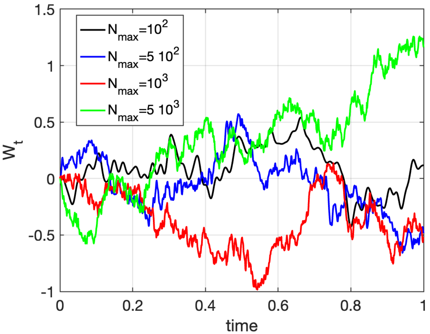
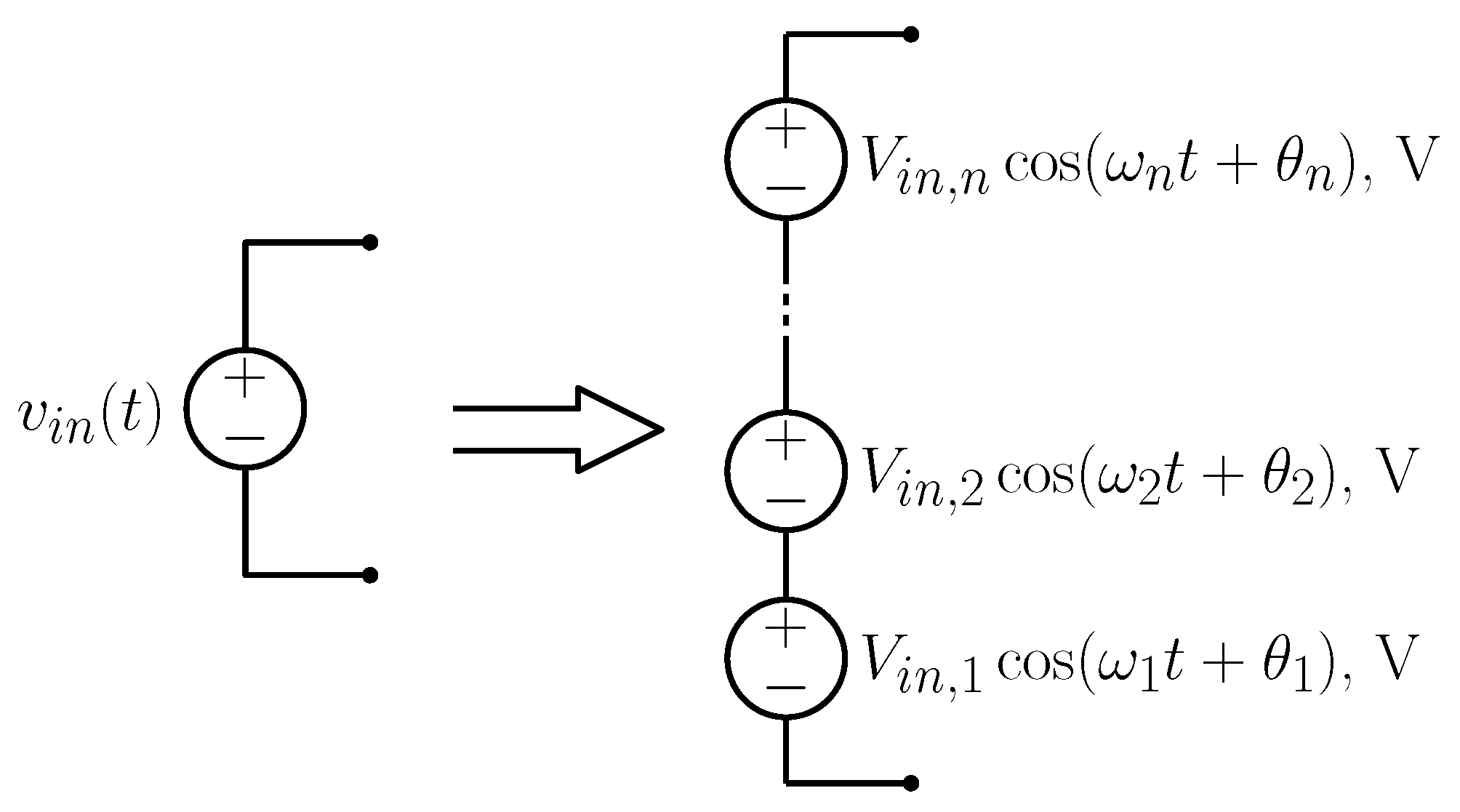
2.1. Modeling Ambient Mechanical Vibrations

The energy of ambient vibrations is typically dispersed over a wide frequency range, making efficient exploitation a challenging task. However, if most of the energy is concentrated in a relatively narrow frequency interval, the force acting on the energy harvester due to ambient vibrations can be modeled as a simple harmonic excitation [28,29,30,31],

$$f_m\left(t\right)=Acos\left(\omega t\right)$$

(1)

where A and $\omega$ are the vibration amplitude and frequency, respectively. A major advantage of assuming a single harmonic excitation, is that the theory of periodically driven oscillators, both linear and nonlinear, is well developed. Ad hoc sophisticated techniques exist for their analysis, both in the time and the frequency domains [32,33,34,35].

Real world vibrations are random in nature, thus, suggesting that they should be modeled as stochastic process. Therefore, it is appropriate to recall some basic concepts about stochastic processes and stochastic calculus.

Let $(\mathbf{\Omega },\mathcal{F},P)$ be a probability space, where $\mathbf{\Omega }$ is the sample space (e.g., the set of all possible outcomes of a given experiment), $\mathcal{F}={\left({\mathcal{F}}_t\right)}_{t\ge 0}$ is a filtration (e.g., the $\sigma$-algebra of all the events), and P is a probability measure (a real function $P:\mathcal{F}\to [0,1]$ such that $P(⌀)=0$ and $P(\mathbf{\Omega }=1$) [36,37]. A real valued random variable $\xi :\mathbf{\Omega }\mapsto \mathbb{R}$ is a measurable function from the sample space $\mathbf{\Omega }$ to the measurable space $\mathbb{R}$, and a vector valued stochastic process ${\mathbf{X}}_t:\mathbf{\Omega }\mapsto {\mathbb{R}}^d$ is a vector of random variables parametrized by $t\in T$. The parameter space T is usually the half-line $[0,+\infty ]$. Alternatively, the stochastic process can be thought of as the function ${\mathbf{X}}_t:\mathbf{\Omega }\times T\mapsto {\mathbb{R}}^d$.

A straightforward method to generate stationary stochastic processes, dating back to the seminal work of Rice [38], is to consider a linear combination of periodic functions

$$X\left(t\right)=\sum _{k=1}^n{\sigma }_k\left(A_{k}cos\left({\omega }_{k}t\right)+B_{k}sin\left({\omega }_{k}t\right)\right)$$

(2)

where ${\sigma }_k$ are constants, and $A_k$, $B_k$ are Gaussian distributed, uncorrelated random variables, with zero expectation value and unit variance. Different criteria have been proposed for the selection of the angular frequencies ${\omega }_k$ [39]. To guarantee that the process is not periodic, it is sufficient that ${\omega }_m/{\omega }_n$ is not rational, for at least one pair $m,n\in \mathbb{N}$ (From the implementation point of view, this condition is never satisfied, as the finite precision of digital computers implies that ratio ${\omega }_m/{\omega }_n$ is always rational. For practical purposes, however, it is sufficient to consider a large enough value for $m/n$). Accordingly, the stochastic process (2) shows zero expectation and the following, stationary auto-correlation function:

$$R(t_1,t_2)=E\left[X\left(t_1\right)X\left(t_2\right)\right]=\sum _{k=1}^n{\sigma }_k^{2}cos\left({\omega }_k(t_1-t_2)\right)$$

(3)

where $E[·]$ denotes the expectation operator. By the Wiener–Khinchin theorem, the corresponding power spectral density is the Fourier transform of the auto-correlation function [36], that reads

$$S\left(\omega \right)=\sum _{k=1}^n{\displaystyle \frac{{\sigma }_k^2}{2}}\left(\delta (\omega -{\omega }_k)+\delta (\omega +{\omega }_k)\right)$$

(4)

where $\delta (·)$ is the Dirac delta function, leading to a representation of the vibration forcing term as a superposition of harmonic components characterized by the frequency set $\left\{{\omega }_k\right\}$, $k=1,\dots ,n$.

The above ideas can be made more rigorous through stochastic expansions and the Karhunen–Loeve representation theorem [40,41]. In the Karhunen–Loeve expansion, a scalar, centered stochastic process $X_t$ is represented on a finite interval $t\in [a,b]$ via a sequence of independent simple random variables, according to:

$$X\left(t\right)=\sum _{i=1}^{+\infty }\sqrt{{\lambda }_i}{\xi }_i{u}_i\left(t\right)$$

(5)

where $\left\{{\xi }_i\right\}$ is a set of mutually uncorrelated random variables to be determined, and $\left\{{\lambda }_i\right\}$, $\left\{u_i\left(t\right)\right\}$, are the sets of eigenvalues and deterministic orthonormal eigenfunctions of the eigenvalue problem [40,41]:

$${\int }_a^{b}R(t_1,t_2)u_i\left(t_2\right)d{t}_2={\lambda }_i{u}_i\left(t_1\right),t_1\in [a,b]$$

(6)

For example, the scalar Wiener process $W\left(t\right)$, characterized by zero mean $E\left[W\right(t\left)\right]=0$, correlation $R(t_1,t_2)=E\left[W\left(t_1\right)W\left(t_2\right)\right]=min(t_1,t_2)$, and normal distribution centered at zero, can be represented on the finite time domain $t\in [0,1]$ by

$$W\left(t\right)=\sqrt{2}\sum _{i=1}^{+\infty }{\xi }_i\frac{sin\left({\lambda }_{i}t\right)}{{\lambda }_i}$$

(7)

where ${\lambda }_i=(i-1/2)\pi$, and $\left\{{\xi }_i\right\}$ are independent normally distributed random variables with zero mean and unit variance, ${\xi }_i\sim \mathcal{N}(0,1)$, where symbol ∼ means “distributed as”. Obviously, for computational purposes, the sum has to be truncated to a suitable number $N_{\max }$ of basis functions. Figure 1 shows the approximation of a Wiener process obtained from (7) with different numbers of basis functions. To date, this approach is fundamental in uncertainty quantification problems [42,43].

An alternative approach for modeling random vibrations is to apply stochastic calculus and the theory of stochastic differential equations (SDEs) [36,37]. A d-dimensional system of SDEs driven by the one-dimensional Wiener process $W_t$ is (Standard notation used in probability is adopted: Capital letters denote random variables, lower case letters denote their possible values. Furthermore, the independent variable (t in this case) is represented at the subscript).

$$d{\mathbf{X}}_t=\mathbf{a}\left({\mathbf{X}}_t\right)dt+\mathbf{B}\left({\mathbf{X}}_t\right)d{W}_t$$

(8)

where the vector valued functions $\mathbf{a}:{\mathbb{R}}^d\mapsto {\mathbb{R}}^d$, $\mathbf{B}:{\mathbb{R}}^d\mapsto {\mathbb{R}}^d$, are called the drift and diffusion terms, respectively. They are measurable functions satisfying a global Lipschitz and a linear growth condition, to enforce the existence and uniqueness solution theorem [37]. If function $\mathbf{B}\left({\mathbf{X}}_t\right)$ is constant, then the noise is said to be un-modulated or additive; otherwise, it is called modulated or multiplicative.

If vibrational energy is distributed over a sufficiently broad spectral interval, ambient vibrations can be modeled by white Gaussian noise, the “formal” derivative of the Wiener process $W_t$. Clearly, a truly white noise process is a physically unrealistic idealization, as the indefinitely flat power spectrum assumption would imply an infinite power content. As a matter of fact, the energy of ambient mechanical vibrations is, in many cases, concentrated at low frequencies. Thus, a low-pass filtered white Gaussian noise can be considered a more realistic model for parasitic vibrations [44,45]. Consider the low-pass filter circuit shown in Figure 2, where the voltage source is a white Gaussian noise process: $v_{in}\left(t\right)=d{W}_t/dt$. Let $\tau =R_f{C}_f$ be the time constant of the circuit. The output voltage $v_{out}\left(t\right)$ is the solution of the Itô SDE (Since the noise is un-modulated (additive), the SDE can be interpreted as either Stratonovich or Itô without any ambiguity [36,37].)

$${\displaystyle \frac{d{v}_{out}}{dt}}=-{\displaystyle \frac{1}{\tau }}{v}_{out}+{\displaystyle \frac{d{W}_t}{dt}}$$

(9)

The voltage $v_{out}\left(t\right)$, solution of (9), is called Ornstein–Uhlenbeck process (OUP). It is characterized by the expectation

$$E\left[v_{out}\left(t\right)\right]=v_{out}\left(0\right)e^{-t/\tau }$$

(10)

where $v_{out}\left(0\right)$ is a deterministic initial condition, and by the stationary time correlation function

$$R_{OUP}(t,t+s)=E\left[v_{out}\left(t\right)v_{out}(t+s)\right]={\displaystyle \frac{1}{2\tau }}{e}^{-\left|s\right|/\tau }$$

(11)

By the Wiener–Khinchin theorem [36], the power spectral density (PSD) is the Fourier transform of the correlation function, so that the PSD for a white Gaussian noise is constant over all frequencies. For the OUP $v_{out}\left(t\right)$ we have

$$S_{OUP}\left(\omega \right)={\displaystyle \frac{1}{1+{\tau }^2{\omega }^2}}$$

(12)

i.e., a Lorentzian spectrum.

2.2. Modeling Vibration Energy Harvester Architectures

The typical energy harvester for ambient mechanical vibrations is composed of an oscillating structure, responsible for capturing vibrational kinetic energy, and a transducer that converts kinetic energy into usable electrical power. The oscillating structure can be a spring, a membrane or a cantilever beam, connected to an inertial mass to enhance the oscillation amplitude [12,16,17,18,46,47,48,49]. Assuming that the mass of the structure is negligible with respect to the inertial mass, and that the motion occurs at least approximately in a straight line, the equation of motion for the mechanical part reads

$$m\ddot{x}+U^{\prime }\left(x\right)+\gamma \dot{x}=f_m\left(t\right)-f_{tr}\left(t\right)$$

(13)

where m is the inertial mass, x is the displacement with respect to the rest position, the dot denotes the derivative with respect to time, $U\left(x\right)$ is an energy (elastic) potential, symbol ${}^{\prime }$ denotes derivative with respect to the argument (in this case, position x), and $\gamma$ is a damping constant. On the right hand side, $f_m\left(t\right)$ is the external force describing ambient vibrations, while $f_{tr}\left(t\right)$ are the forces exerted by the transducer responsible for the mechanical to electrical power conversion.

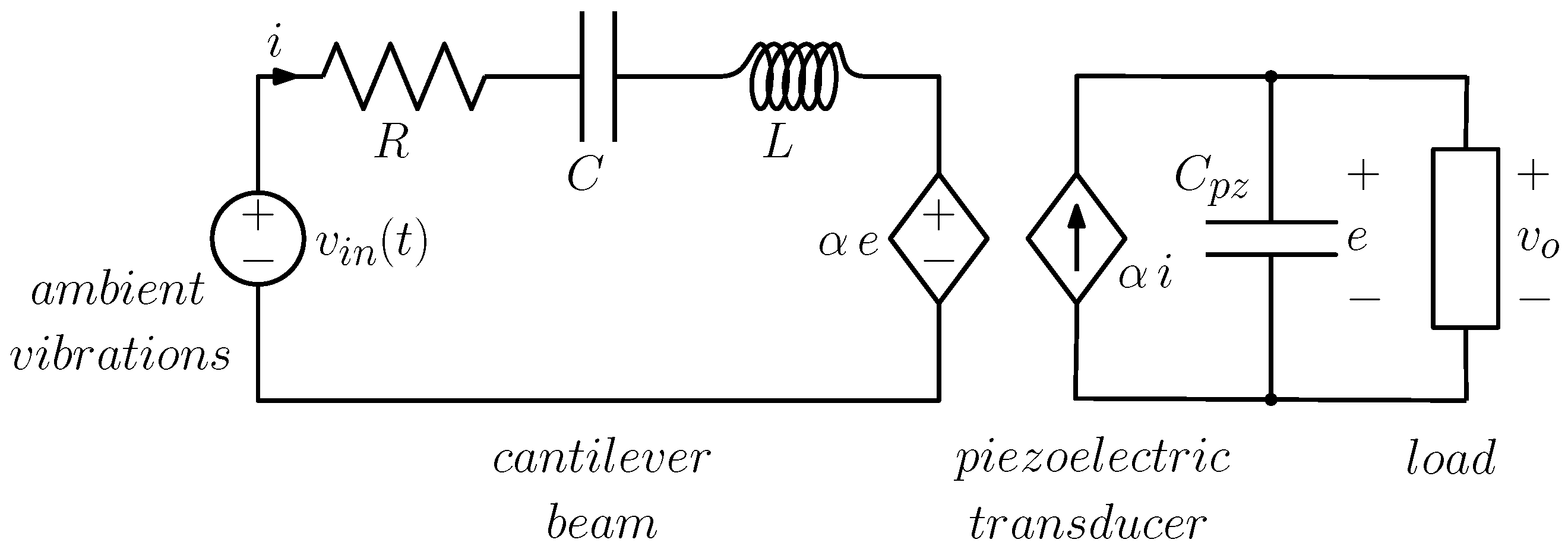
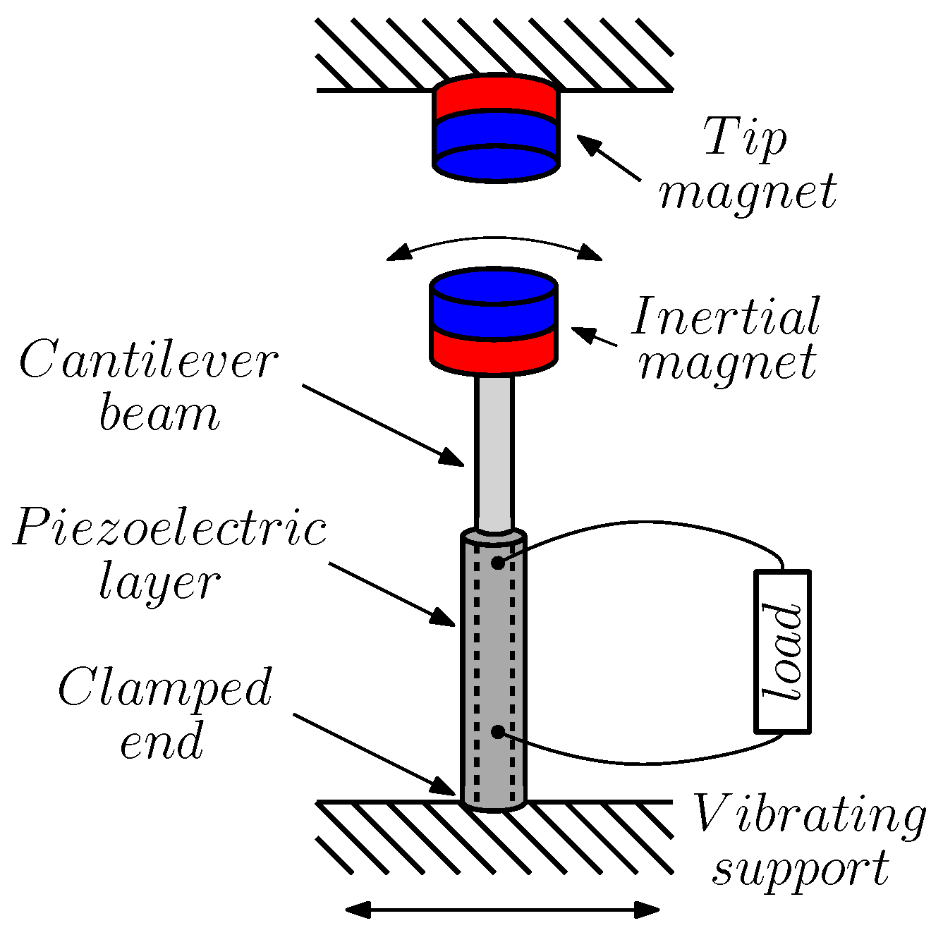
2.2.1. Piezoelectric Harvesters

Piezoelectric transducers rely upon piezoelectric materials to convert mechanical stress and strain induced by oscillations into electrical power. Piezoelectric transducers offer good efficiency, they are relatively cheap and, more importantly, they are easy to miniaturize [50].

The governing equations for a piezoelectric transducer can be derived from the characteristic equations of piezoelectric materials [12,51,52]

$$\begin{array}{cc}\hfill S_{ij}=& s_{ijkl}^E{T}_{kl}+d_{kij}{E}_k\hfill \end{array}$$

(14a)

$$\begin{array}{cc}\hfill D_i=& d_{ikl}{T}_{kl}+{\epsilon }_{ik}^T{E}_k\hfill \end{array}$$

(14b)

linking the mechanical strain $S_{ij}$ (rank two tensor) and the dielectric charge displacement $D_i$ (rank one tensor) to the mechanical stress $T_{kl}$ (rank two tensor) and the electric field $E_k$ (rank one tensor). The linear transformation is defined by:

• the compliance tensor $s^{\mathit{E}}$, defined for a constant electric field as the strain generated per unit stress;
• the tensor d of piezoelectric charge constants
• the absolute permittivity ${\epsilon }^T$, namely the dielectric displacement per unit electric field for constant stress [12]

Equation (14) provides a link among microscopic, local (i.e., space-dependent) physical variables, while an effective modeling of the piezoelectric material calls for the derivation of a lumped description, that can be obtained through spatial integration of the local variables. For a single degree of freedom (DOF) mechanical system (the usual approximation) characterized by the scalar spatial displacement x, the lumped equations for the piezoelectric material in quasi-static conditions read

$$\begin{array}{cc}\hfill f_{tr}\left(t\right)& =\alpha e\left(t\right)\hfill \end{array}$$

(15a)

$$\begin{array}{cc}\hfill q\left(t\right)& =\alpha x\left(t\right)-C_{pz}e\left(t\right)\hfill \end{array}$$

(15b)

where $f_{tr}\left(t\right)$ is the force exerted by the transducer, $\alpha$ is the electro-mechanical coupling factor (in N/V or As/m), $C_{pz}$ is the electrical capacitance of the piezoelectric layer, $q\left(t\right)$ is the electrical charge, and $e\left(t\right)$ is the output voltage of the piezoelectric transducer.

Figure 3 shows the representation of the piezoelectric transducer as an electromechanical two-port network, with mechanical quantities at the input (left port) and electrical quantities at the output (right port), and closed on an electrical load.

The lumped parameter model (15) implies that the same coupling constant $\alpha$ is used for both mechanical-to-electrical and electrical-to-mechanical conversion. Consequently, dissipation in the mechanical part is accounted for by the damping coefficient $\gamma$. The piezoelectric transducer is assumed to be a lossless two port element, that transfers energy from the mechanical part to the electrical load, and vice-versa. Such a model has been extensively used in literature [21,31,53,54,55,56].

2.2.2. Electromagnetic Induction Harvesters

Electromagnetic energy harvesters exploit magnetic induction to convert mechanical power into electrical power. The oscillating structure is typically composed of a magnet, either connected to a vibrating support through springs or suspended by a magnetic field generated by other magnets, and placed inside a coil [57,58,59,60]. Vibrations of the support produce oscillations of the suspended magnet, inducing a current in the surrounding coil through Faraday’s law.

The transducer force corresponds to a transversal component of the electromagnetic Lorentz force, generated by the current induced in the coil

$${\mathbf{F}}_L=I\oint \mathbf{B}\times d\mathbf{s}$$

(16)

where I is the induced current, $d\mathbf{s}$ is the differential length vector along the inductor coil, and $\mathbf{B}$ is the magnetic field. Application of Kirchhoff voltage law yields

$$L_C\dot{I}+v_o+v_e=0$$

(17)

where $L_C$ is the inductance of the generator coil, $v_o$ is the voltage across the load and $v_e$ is the electromotive force, given by

$$v_e=-{\displaystyle \frac{d}{dt}}{\int }_S\mathbf{B}·\mathit{n}dA$$

(18)

where $\mathit{n}$ is the transversal unit vector for the coil cross-section S. For a N turn induction coil the Lorentz force and the electromotive force are then given by [58]

$$F_L=2\pi r_c\left(\sum _{j=1}^N{B}_{r_j}\right)I{v}_e=-2\pi r_c\left(\sum _{j=1}^N{B}_{r_j}\right)\dot{x}$$

(19)

Here, $r_c$ is the radius of the generating coil and $B_{r_j}$ is the radial magnetic field at location x of coil j. The magnetic field can be evaluated exploiting standard methods, such as finite or boundary element techniques. In general, the electro-mechanical coupling coefficient $B_L\left(x\right)=2\pi r_c\left({\sum }_{j=1}^N{B}_{r_j}\right)$ depends on the position of the magnet. A great simplification is obtained by assuming small oscillations of the magnet, thus approximating $B_L\left(x\right)$ with its value when the spring is at the rest position [58].

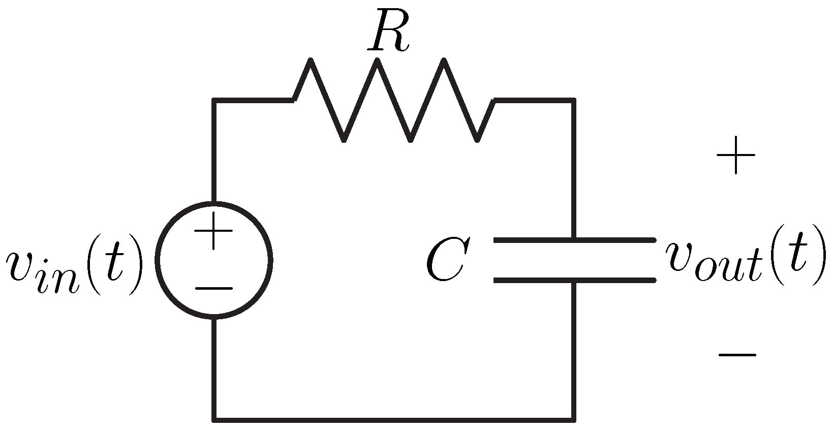
2.3. Equivalent Circuit Models

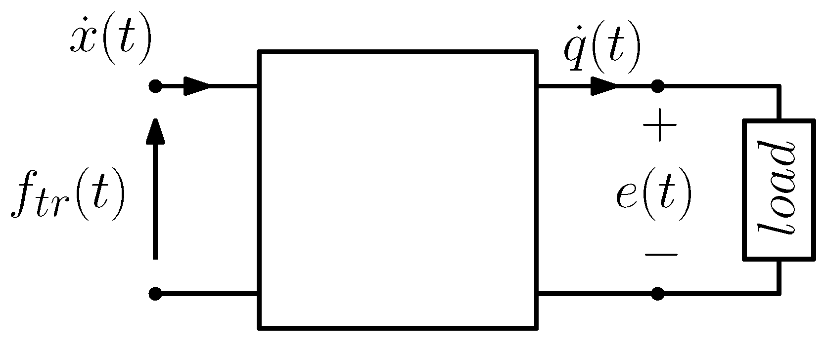
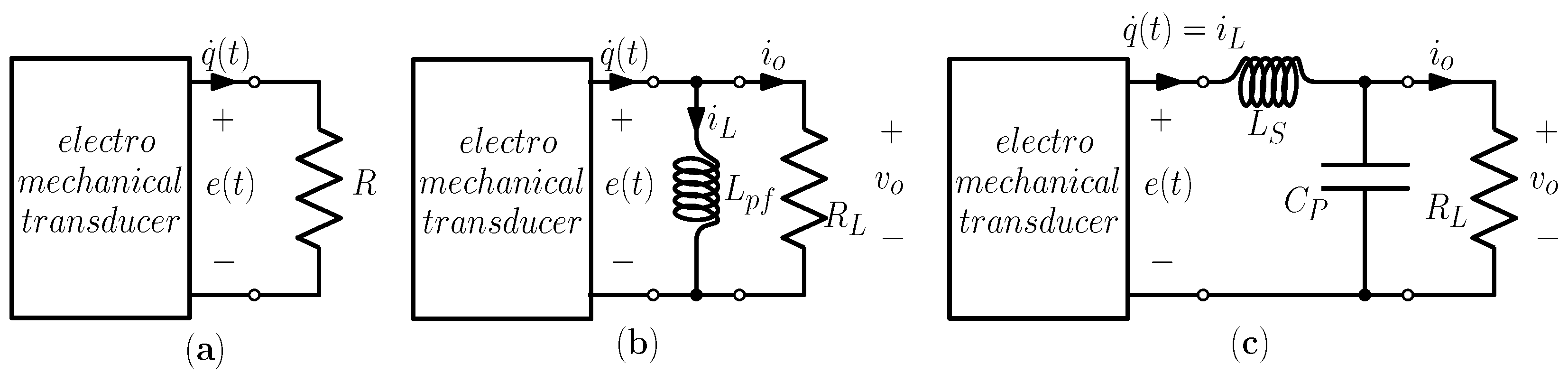
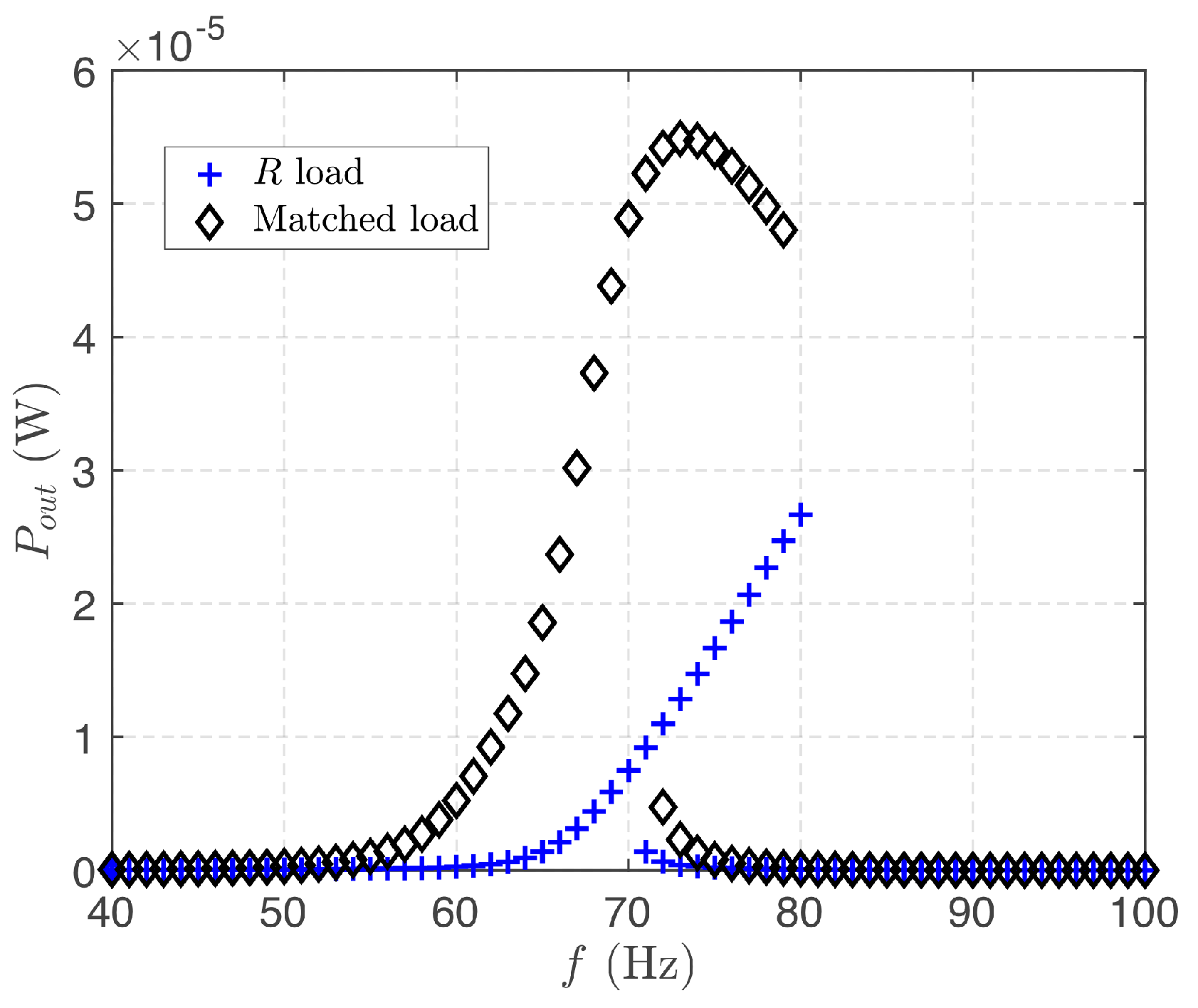
The use of electrical to mechanical analogies can be traced back to the very beginning of studies of electro-mechanical phenomena, when they were used to describe the relatively novel electrical phenomena in terms of better understood mechanical problems. As the understanding of electrical phenomena progressed, and especially after the development of lumped parameter circuit models, the use of the analogies was reversed, as it was realized that many problems in mechanics can be described by equivalent circuits, and that concepts and methods of electrical network theory can be applied for their solution. Today, equivalent circuits are commonly used to describe multi-domain structures [61,62,63], biological systems [64] and even quantum mechanical phenomena [65,66].

The term equivalent refers to a circuit that retains all the characteristics of a given system and, in particular, that is described by the same set of state equations. Equivalent circuits for energy harvesters are conveniently derived replacing mechanical variables, like force, velocity and so on, with electrical quantities, like voltage, current, etc., as summarized in

Table 1. Mechanical-electrical analogy.

Mechanical	Electrical
Force, f	Voltage, v
Displacement, x	Charge, q
Momentum $m\dot{x}$	Flux linkage, $\phi$
Mass, m	Inductance L
Compliance, $k^{-1}$	Capacity, C
Damping, $\gamma$	Resistance, R

.

Using mechanical to electrical analogies, Equations (13) and (14) or (13)–(17) can be rewritten in terms of electrical quantities. Interpreting the resulting equations as Kirchhoff voltage and current laws, the equivalent circuits shown in Figure 4 and Figure 5 can be obtained, respectively.

2.4. Load Modeling

In circuit theory, a load is any circuit element that absorbs power from the rest of the circuit. In energy harvesting applications, the load is commonly modeled as a resistor (see Figure 6a).

For the piezoelectric harvester, application of Ohm law gives $\dot{q}\left(t\right)=Ge\left(t\right)$ ($G=1/R$ is the load conductance). The governing equations for a piezoelectric energy harvester with resistive load are obtained rewriting (13) as a system of first order differential equations, and using (15), thereby obtaining:

$$\begin{array}{cc}\hfill \dot{x}=& y\hfill \end{array}$$

(20a)

$$\begin{array}{cc}\hfill \dot{y}=& -{\displaystyle \frac{1}{m}}{U}^{\prime }\left(x\right)-{\displaystyle \frac{\gamma }{m}}y-{\displaystyle \frac{\alpha }{m}}e+{\displaystyle \frac{1}{m}}{f}_m\left(t\right)\hfill \end{array}$$

(20b)

$$\begin{array}{cc}\hfill \dot{e}=& {\displaystyle \frac{\alpha }{C_{pz}}}y-{\displaystyle \frac{G}{C_{pz}}}e\hfill \end{array}$$

(20c)

Similarly, the governing equations for an electromagnetic energy harvester are obtained from (13), and (17)–(19)

$$\begin{array}{cc}\hfill \dot{x}=& y\hfill \end{array}$$

(21a)

$$\begin{array}{cc}\hfill \dot{y}=& -{\displaystyle \frac{1}{m}}{U}^{\prime }\left(x\right)-{\displaystyle \frac{\gamma }{m}}y-{\displaystyle \frac{B_L}{m}}I+{\displaystyle \frac{1}{m}}{f}_m\left(t\right)\hfill \end{array}$$

(21b)

$$\begin{array}{cc}\hfill \dot{I}=& {\displaystyle \frac{B_L}{L_C}}y-{\displaystyle \frac{G}{L_C}}I\hfill \end{array}$$

(21c)

It is clear that (20) and (21) are completely equivalent. Therefore, for the sake of simplicity, hereinafter only piezoelectric energy harvesters shall be considered.

As mentioned in Section 2.3, one of the main advantages of using equivalent circuits, is the inheritance of concepts and methods from circuit theory. In particular, the maximum average power transfer theorem states that, in an AC circuit, maximum power is transferred from the source to the load if the impedance of the latter is the complex conjugate of the source impedance. Consider the circuits in Figure 4 and Figure 5. A resistive load can match the circuit impedance, defined at the left of the load if, and only if, the harvester is working at the resonant frequency. Otherwise, including the case of a multi-frequency source, the harvested power drops significantly because of the impedance mismatch.

In vibration energy harvesting, impedance mismatch is a limiting key factor, because ambient vibrations have relatively low frequencies, variable from few tens to few hundred Hz, whereas the electrical domain has a higher resonant frequency, thus resulting in a significant impedance mismatch. Several works have suggested that power factor correction can be applied to improve the performances of energy harvesters [31,55,56]. Power factor correction is a standard method of electrical engineering, that permits increasing the average power absorbed by the load, and reducing the lag between the voltage across and the current through the load. For a piezoelectric energy harvester, given the capacitive reactance of piezoelectric transducers, power factor correction is obtained by inserting an inductive element in parallel with the resistive load, as shown in Figure 6b. Conversely, for an electromagnetic energy harvester, the inductive reactance of the coil can be compensated for by connecting a capacitor in series with the resistive load.

An alternative solution, proposed in [45,67], amounts to interposing an impedance matching network between the transducer and the load, as shown in Figure 6c. The matching network not only quenches the impedance mismatch, but it can also be designed to resonate at a chosen frequency, not necessarily coincident with the resonant frequency of the energy harvester. This characteristic is very useful when the resonant frequency of the energy harvester and the frequency where vibration energy is concentrated are far apart [67].

There are many different types of matching networks, which differ in the number of electrical components and their interconnections. The simplest matching stage is the L-network, composed of two reactive components (inductor and capacitor), arranged to form an L shaped structure. In total, eight different arrangements for the L-network are possible. Figure 6 shows one of the possible setups, known as the low-pass L-matching network, that is well suited for piezoelectric energy harvesters [45,67]. The matching network is low-pass because at very low frequencies the inductor is equivalent to a short circuit (and the capacitor, to an open circuit). This is a particularly desirable feature because, in general, most of the energy of ambient mechanical vibrations is concentrated at low frequencies.

Figure 7 shows an example, taken from [67], of the benefits of the application of a matching network. The figure represents the average output power as a function of the forcing frequency for a cantilever beam piezoelectric energy harvester. Blue crosses are the results with a resistive load, while black diamonds refer to the use of a matching network, demonstrating an about 80% increase of the power transferred to the load.

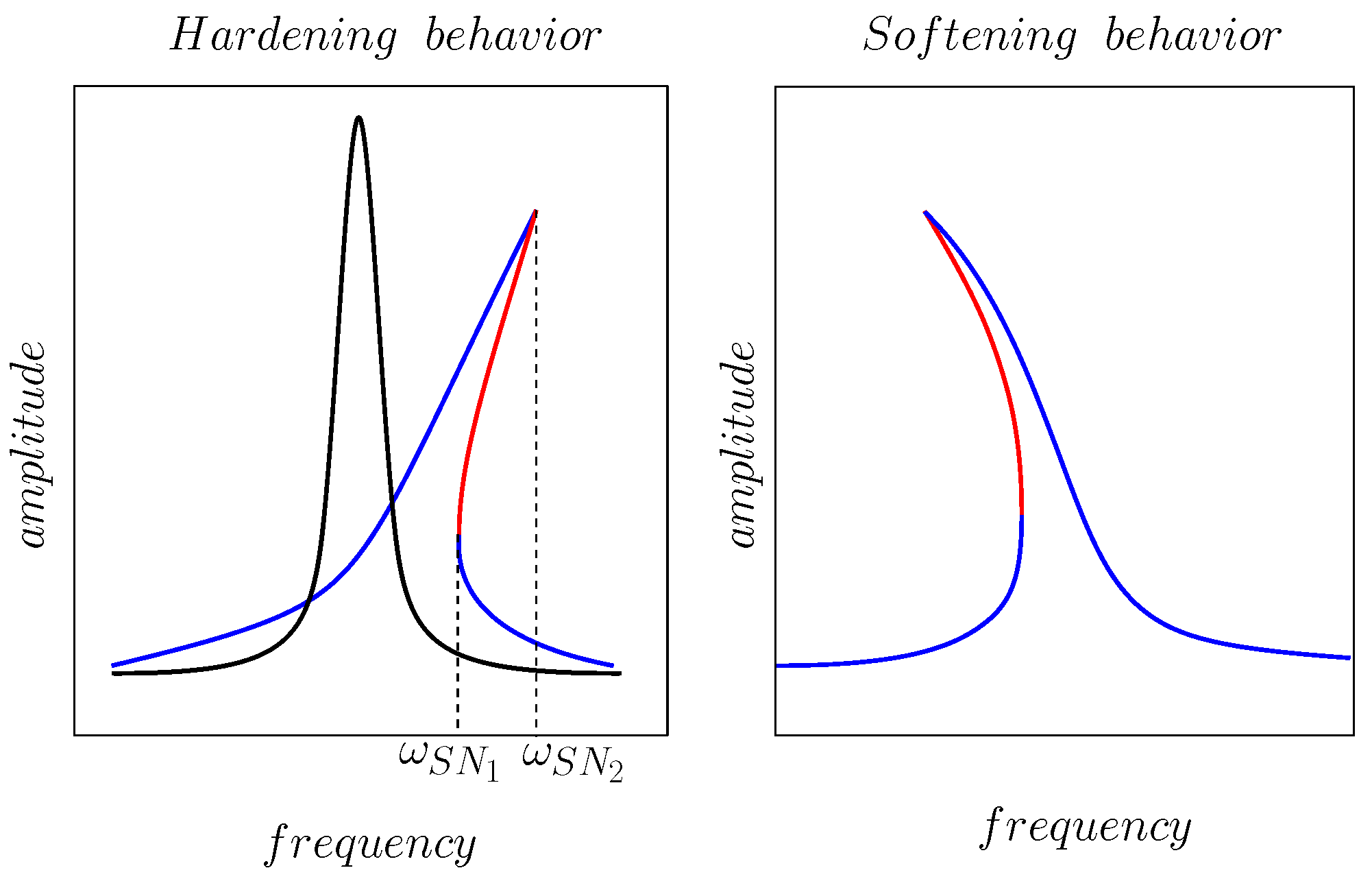
2.5. Nonlinear Harvester Modeling

Irrespective of the working principle, energy harvesters operate as resonators. For a linear harvester and harmonic external excitation with fixed frequency, maximum energy is transferred from the environment to the electric load tuning one of the harvester modal frequencies, usually the first, to be equal, or at least as close as possible, to the excitation frequency.

Working close to the resonance maximizes the oscillation amplitude, but it entails a limited operating band. In fact, linear harvesters are designed as high Q-factor resonators, with amplitude response rapidly decreasing around the resonance peak. Manufacturing tolerances, parameter inaccuracies and excitation variations, in general, all contribute to de-tuning the resonator, further reducing the already limited energy output.

The limited band issue becomes fundamental if one considers that ambient vibrations are more realistically described as random process, often non-stationary, either with a wide frequency spectra, or with a dominant frequency that changes with time [21]. Therefore, tuning the resonator becomes unfeasible, significantly dampening the performances of linear harvesters.

To tackle the problem, linear harvesters with tunable response have been proposed [68,69,70,71,72]. In particular, mechanical filters made by cascade connected inertial masses were considered in [69]. In [71,72], the authors proposed mechanical systems with self adjustable resonance frequency, achieved by an inertial mass free to slide along the oscillating beam. The moving mass settles to a position such that the resonant frequency of the cantilever beam matches the frequency of the external forcing.

An alternative solution amounts to including nonlinearities in the system, as a means to broaden the response of the resonator. Nonlinearity may arise as a consequence of material properties, for example taking into account the nonlinear strain deflection relationships due to large deformations, or from a nonlinear electro-mechanical coupling mechanism, as in the nonlinear constitutive relationships of piezoelectricity [73]. The benefit of these nonlinearities is to produce a “bending” of the amplitude response introducing a hysteretic behaviour, trading off the efficiency at the resonant frequency for a larger bandwidth, as illustrated in Figure 8. Figure 9 shows an example of the hysteretic behaviour typical of nonlinear harvesters as obtained by applying the harmonic balance analysis technique described in Section 3.2. Data represent the root mean square value of the output voltage for the nonlinear cantilever beam piezoelectric energy harvester in [67], subject to a periodic forcing, vs. the input vibration frequency. Blue crosses, blue × and red pentagrams are for the resistive load. Black squares, black circles and red diamonds are for the matched load. Blue and black markers refer to stable limit cycles, red markers are for unstable limit cycles.

Nonlinearity can also be intentionally introduced by design, with the obvious advantage of controlling the degree and magnitude of the nonlinearity itself. For instance, a softening spring behaviour can be introduced, through application of electrostatic potential [74] or smart magnet positioning [75]. The softening spring effect is analogous to what is described above: to produce a bending of the resonant curve with consequent hysteresis and, thus, bandwidth enlargement. The only difference is that the resonant frequency is shifted toward lower values, as shown in the right part of Figure 8, which may be preferable in energy harvesting low frequency applications [76].

In piezoelectric cantilever-based energy harvesters, the most common solution consists of using a magnetic material as the inertial mass, and in placing another magnet on a fixed support right in front, with polarities opposed to those of the tip magnet, to create a biased inverted pendulum and a magnetic repulsive force [19]. A schematic representation is given in Figure 10. Assuming again a single degree of freedom description, when the distance between the magnets is large enough, the cantilever beam behaves as a linear oscillator. The system is subject to a quadratic elastic potential, and, in the absence of external forcing, it exhibits a single equilibrium point corresponding to the vertical rest position.

Conversely, when the distance between the two magnets is small enough, the system is subject to a nonlinear elastic force. Magnetic repulsion forces the beam to the left or to the right of the vertical position. The unforced system exhibits bi-stability, with two stable equilibrium points, each with its own basin of attraction, separated by an unstable saddle, corresponding to the vertical rest position. For small external forcing, the beam oscillates either around the left or the right equilibrium position (see Figure 11, on the left), depending on the initial condition. For small amplitude oscillations, the system can still be described in terms of a linear oscillator, with a resonant frequency higher than in the previous case [19], and the stationary distribution shows two well separated peaks located around the stable equilibrium points (Figure 11, right).

If the magnitude of the external forcing is increased, oscillations around each of two equilibrium points are alternated by large excursions from one basin of attraction to the other, as shown in the left part of Figure 12. Correspondingly, the two peaks in the stationary distribution merge and partially overlap. The irregular large excursions correspond to oscillations with larger amplitudes, that induce higher deformation of the beam collecting more energy. For high noise intensity, the system exhibits more and more frequent excursions from the basin of attraction of one equilibrium to the other, with a motion that resembles a random wandering around the unstable saddle, as depicted in Figure 13, left. In correspondence, the merging of the two peaks of the stationary distribution is more pronounced, so as to take the shape a multivariate normal distribution (Figure 13, right).

The figures were obtained through numerical integration of the SDEs for a bi-stable energy harvester with cubic nonlinearity and resistive load, subject to a random force modeled as white Gaussian noise. The equations were integrated numerically using the Euler–Maruyama numerical integration scheme, see Section 3.4. For the stationary distributions, the probability to find the system in the state $(x+dx,y+dy)$ is estimated as the number of samples in that interval, divided by the total number of samples.

The idea to exploit multi-stability was further developed and generalized, introducing tri-stable [77,78,79] and, more generally, multi-stable energy harvesters [80,81,82,83,84,85]. In [77] it was shown that a tri-stable arrangement passes easily through potential wells, generating higher energy output over a wider range of frequency with respect to a bi-stable setup with a deeper potential well. In [79], a tri-stable system was designed, with multiple magnets and springs, exploiting a rotatable magnet–spring oscillating system. It was shown that such a solution not only reduced the potential energy barrier and the threshold of snap-through, but also broadened the bandwidth of inter-well motion. In [80], an ingenious setup, where the inertial mass on the top of a cantilever beam is connected to a support through three springs, was proposed. The resulting structure exhibits four steady state responses and dozens of primary resonance modes. Another interesting design, composed of a moving magnet connected to the supports by two linear springs and surrounded by four fixed small magnets was proposed in [84]. The common denominator of these works was the introduction of structures designed to produce a nonlinear elastic potential $U\left(x\right)$ that exhibits three or more minima. In this way, hops among the different wells correspond to oscillations of larger amplitude, producing enhanced mechanical strain and, thus, more electrical power.

3. Analysis

The models of energy harvesting systems introduced in Section 2 can be classified into two categories: linear and nonlinear. Furthermore, each class can be further divided into deterministic (periodically forced) or stochastic. The methods and techniques for their analysis are those of dynamical systems theory. Dynamical systems form a very rich research area, that in the last few decades has witnessed an explosive growth, thanks to the rapidly developing topics of nonlinear dynamics, bifurcations, chaos, and complex systems in general. A comprehensive review of the concepts and methods of dynamical system theory is far beyond the scope of the present paper. Here, only some methods that have been successfully applied to the analysis of vibration energy harvesting systems are discussed.

3.1. Frequency Domain Methods for Linear Systems

Frequency domain techniques are classical tools for the analysis of both linear and nonlinear circuits and systems. If mechanical vibrations are modeled by the simple harmonic signal (1), then the voltage source in the AC circuit in Figure 4 can be conveniently described by its phasor ${\widehat{F}}_m\left(\omega \right)$, a complex number including amplitude and phase. Using phasor analysis, the output voltage reads

$${\widehat{V}}_o\left(\omega \right)=H\left(\omega \right){\widehat{F}}_m\left(\omega \right)$$

(22)

where ${\widehat{V}}_o\left(\omega \right)$ is the phasor of the output voltages, and $H\left(\omega \right)$ is the AC circuit’s transfer function (possibly including the power-factor correction network or the matching stage in Figure 6). The average input and output powers read

$$\begin{array}{cc}\hfill P_{in}=& \frac{1}{2}\mathrm{Re}\left[Y_{in}\left(\omega \right)\right]{\left|{\widehat{F}}_m\left(\omega \right)\right|}^2\hfill \end{array}$$

(23a)

$$\begin{array}{cc}\hfill P_{out}=& \frac{1}{2}{G\left|H\left(\omega \right)\right|}^2{\left|{\widehat{F}}_m\left(\omega \right)\right|}^2\hfill \end{array}$$

(23b)

where $\mathrm{Re}[·]$ denotes the real part, and $Y_{in}\left(\omega \right)$ is the circuit input admittance. The power efficiency is

$$\eta ={\displaystyle \frac{P_{out}}{P_{in}}}=G{\displaystyle \frac{{\left|H\left(\omega \right)\right|}^2}{\mathrm{Re}\left[Y_{in}\left(\omega \right)\right]}}$$

(24)

The extension to multi-periodic inputs is straightforward. Using mechanical to electrical analogies, a mechanical force, such as those represented by (2) or (5), is replaced by a set of series-connected voltage sources, as illustrated in Figure 14. The output voltage can be computed applying the superposition principle, considering one source at a time. The output voltage phasor is found using (22), where the transfer function is calculated at each frequency ${\omega }_k$. Interestingly, because frequencies are all different, both the input and the output powers are decomposed as the sum of the contributions of each source.

Frequency domain techniques can also be applied to a fully stochastic input. In this case, the energy harvester is interpreted as a linear time invariant system (LTI) subject to a random input $x\left(t\right)$ [45]. The input–output relation for LTI systems is

$$y\left(t\right)={\int }_{-\infty }^{+\infty }x(t-r)h\left(r\right)dr=h\left(t\right)\ast x\left(t\right)$$

(25)

where $h\left(t\right)$ is the impulse response, $y\left(t\right)$ is the system output, and symbol ∗ denotes the convolution product. The autocorrelation function $R_{yy}\left(\tau \right)$ of the output variable $y\left(t\right)$ is [36]

$$R_{yy}\left(\tau \right)=E\left[y\left(t\right)y(t-\tau )\right]={\int }_{-\infty }^{+\infty }{\int }_{-\infty }^{+\infty }h\left(r\right)h\left(s\right)R_{xx}(\tau +r-s)dsdr$$

(26)

Taking the Fourier transform, the input–output relationship for power spectral densities is obtained

$$S_Y\left(\omega \right)={\left|H\left(\omega \right)\right|}^2{S}_X\left(\omega \right)$$

(27)

where $H\left(\omega \right)=\widehat{Y}\left(\omega \right)/\widehat{X}\left(\omega \right)$ is the system’s transfer function, $\widehat{Y}\left(\omega \right)$, $\widehat{X}\left(\omega \right)$ are the Fourier transforms of output and input, respectively, and $S_X\left(\omega \right)$ is the power spectral density of the input, e.g., the random vibrations. The average power absorbed by the load, calculated using Parseval theorem is

$$P_{out}=GE\left[v_{out}^2\left(t\right)\right]=G{\int }_0^{+\infty }{S}_Y\left(\omega \right)d\omega$$

(28)

and can be easily calculated substituting (27) and calculating the integral.

The main technical difficulty in the application of frequency domain analysis is the need to calculate the transfer function $H\left(\omega \right)$. Finding $H\left(\omega \right)$ may become cumbersome for complex structures, where one or more matching networks or other linear two ports, are connected at the transducer output port. However, as shown in [45], an energy harvester can be represented by cascade-connected electro-mechanical two-ports. As a result, the transfer function can be easily calculated from the overall transmission matrix that, in turn, is evaluated as the matrix product of the partial transmission matrices of each two-port. The approach is particularly well suited to dealing with the case of colored noise, that requires some kind of “preprocessing” of the white Gaussian noise. For example, in the case of the Ornstein–Uhlenbeck process, it is sufficient to include an additional two-port, the low pass filter, in front of the electro-mechanical two-port chain that describes the harvester.

3.2. Frequency Domain Methods for Nonlinear Systems: Harmonic Balance

There are many scientific applications, ranging at least from electrical and microwave engineering to mechanical systems, wherein the main interest lies in the determination of periodic or quasi-periodic solutions of dynamical systems, and the full computation of the solution transient can be discarded altogether. In the frequency domain, this task can be accomplished exploiting the Harmonic Balance (HB) numerical technique. In its essence, HB transforms the differential equations describing the system dynamics into an algebraic system, the unknowns of which are the coefficients of the Fourier series representing the steady-state solution (In autonomous systems, where a time shifted solution is still a valid solution, one of the coefficients can be chosen arbitrarily, while the frequency is unknown. The total number of unknowns for the HB technique remains the same for both autonomous and non-autonomous systems.) [86,87].

For the sake of simplicity, the case of strictly periodic solutions is considered first, and the notation is introduced considering a scalar differential equation like

$$\frac{{\displaystyle \mathrm{d}x}}{{\displaystyle \mathrm{d}t}}=f\left(x\right)+s\left(t\right)$$

(29)

where $x\left(t\right)$ is a real, scalar unknown, $f\left(x\right)$ is a scalar nonlinear function regular enough to allow for a unique solution of (29) once a proper initial condition is defined, and $s\left(t\right)$ is a periodic (period equal to T), scalar forcing term. In these conditions, a T periodic solution $x_{\mathrm{s}}\left(t\right)$ of (29) exists. Due to periodicity, $x_{\mathrm{s}}\left(t\right)$ can be represented in the time domain by means of a trigonometric Fourier series

$$x_{\mathrm{s}}\left(t\right)={\widehat{x}}_{\mathrm{s},0}^{\left(\mathrm{c}\right)}+\sum _{h=1}^{+\infty }\left[{\widehat{x}}_{\mathrm{s},h}^{\left(\mathrm{c}\right)}cos\left(h\omega t\right)+{\widehat{x}}_{\mathrm{s},h}^{\left(\mathrm{s}\right)}sin\left(h\omega t\right)\right]$$

(30)

where ${\widehat{x}}_{\mathrm{s},h}^{\left(\mathrm{c}\right)}$ and ${\widehat{x}}_{\mathrm{s},h}^{\left(\mathrm{s}\right)}$ are, respectively, the cosine and sine amplitudes associated to the h-th harmonic at (angular) frequency $\omega =2\pi /T$. The series is here truncated selecting a finite value for the maximum order $N_{\mathrm{H}}$, a choice entailing an obvious trade-off between accuracy and numerical efficiency. As the amplitudes are real, the truncated Fourier representation is fully defined by $2N_{\mathrm{H}}+1$ real coefficients.

The coefficients of the Fourier development can be traced back to integrals implementing the projection of $x_{\mathrm{s}}\left(t\right)$ on the corresponding harmonic. However a more efficient numerical evaluation can be derived by means of the following approach. Let us discretize the $[0,T]$ fundamental period into a set of $2N_{\mathrm{H}}+1$ time samples $t_k$ ($k=1,\dots ,2N_{\mathrm{H}}+1$). The time samples of $x_{\mathrm{s}}\left(t\right)$ are then collected into vector $\breve{\mathbf{x}}={[x\left(t_1\right),x\left(t_2\right),\dots ,x\left(t_{2N_{\mathrm{H}}+1}\right)]}^{\mathrm{T}}$ (where ${}^{\mathrm{T}}$ denotes the transpose), which is, in turn, in a one-to-one linear relation with the collection of the harmonic amplitudes ${\widehat{\mathbf{x}}}_{\mathrm{s}}={[{\widehat{x}}_{\mathrm{s},0}^{\left(\mathrm{c}\right)},{\widehat{x}}_{\mathrm{s},1}^{\left(\mathrm{c}\right)},{\widehat{x}}_{\mathrm{s},1}^{\left(\mathrm{s}\right)},\dots ,{\widehat{x}}_{\mathrm{s},N_{\mathrm{H}}}^{\left(\mathrm{c}\right)},{\widehat{x}}_{\mathrm{s},N_{\mathrm{H}}}^{\left(\mathrm{s}\right)}]}^{\mathrm{T}}$ expressed by means of the invertible matrix ${\mathbf{\Gamma }}^{-1}$, providing the representation of the discrete Fourier transform (DFT)

$$\breve{\mathbf{x}}={\mathbf{\Gamma }}^{-1}\widehat{\mathbf{x}}⟺\widehat{\mathbf{x}}=\mathbf{\Gamma }\breve{\mathbf{x}}.$$

(31)

Assuming equally spaced time samples, it is possible to express $t_k=kT/(2N_{\mathrm{H}}+1)$ ($k=1,\dots ,2N_{\mathrm{H}}+1$) so that the explicit expression for the DFT operator becomes

$${\mathbf{\Gamma }}^{-1}=\left[\begin{array}{cccccc}1& {\gamma }_{1,1}^{\mathrm{c}}& {\gamma }_{1,1}^{\mathrm{s}}& \dots & {\gamma }_{1,N_{\mathrm{H}}}^{\mathrm{c}}& {\gamma }_{1,N_{\mathrm{H}}}^{\mathrm{s}}\\ 1& {\gamma }_{2,1}^{\mathrm{c}}& {\gamma }_{2,1}^{\mathrm{s}}& \dots & {\gamma }_{2,N_{\mathrm{H}}}^{\mathrm{c}}& {\gamma }_{2,N_{\mathrm{H}}}^{\mathrm{s}}\\ ⋮& ⋮& ⋮& & ⋮& ⋮\\ 1& {\gamma }_{2N_{\mathrm{H}}+1,1}^{\mathrm{c}}& {\gamma }_{2N_{\mathrm{H}}+1,1}^{\mathrm{s}}& \dots & {\gamma }_{2N_{\mathrm{H}}+1,N_{\mathrm{H}}}^{\mathrm{c}}& {\gamma }_{2N_{\mathrm{H}}+1,N_{\mathrm{H}}}^{\mathrm{s}}\end{array}\right]$$

(32)

where ${\gamma }^{\mathrm{c}}$ and ${\gamma }^{\mathrm{s}}$ are given by:

$${\gamma }_{p,q}^{\mathrm{c}}=cos\left(q\omega t_p\right)=cos\left(\frac{{\displaystyle q2\pi p}}{{\displaystyle 2N_{\mathrm{H}}+1}}\right){\gamma }_{p,q}^{\mathrm{s}}=sin\left(q\omega t_p\right)=sin\left(\frac{{\displaystyle q2\pi p}}{{\displaystyle 2N_{\mathrm{H}}+1}}\right).$$

(33)

Notice that ${\mathbf{\Gamma }}^{-1}$ is independent of the period T (or, equivalently, of $\omega$), as a consequence of the chosen time samples.

From (30), one immediately derives

$$\frac{{\displaystyle \mathrm{d}{x}_{\mathrm{s}}}}{{\displaystyle \mathrm{d}t}}={\dot{x}}_{\mathrm{s}}\left(t\right)=0+\sum _{h=1}^{N_{\mathrm{H}}}\left[(-h\omega ){\widehat{x}}_{\mathrm{s},h}^{\left(\mathrm{c}\right)}sin\left(h\omega t\right)+h\omega {\widehat{x}}_{\mathrm{s},h}^{\left(\mathrm{s}\right)}cos\left(h\omega t\right)\right],$$

(34)

the harmonic amplitudes of the first derivative of $x_{\mathrm{s}}\left(t\right)$ take the form of a linear transformation of ${\widehat{\mathbf{x}}}_{\mathrm{s}}$

$${\widehat{\dot{\mathbf{x}}}}_{\mathrm{s}}=\mathbf{\Gamma }{\breve{\dot{\mathbf{x}}}}_{\mathrm{s}}=\mathbf{\Omega }{\widehat{\mathbf{x}}}_{\mathrm{s}}$$

(35)

where $\mathbf{\Omega }$ is the representation of the derivative operator in the Fourier domain, namely the tri-diagonal matrix

$$\mathbf{\Omega }=\omega \left[\begin{array}{cccccccc}0& 0& 0& 0& 0& \dots & 0& 0\\ 0& 0& 1& 0& 0& \dots & 0& 0\\ 0& -1& 0& 0& 0& \dots & 0& 0\\ 0& 0& 0& 0& 2& \dots & 0& 0\\ 0& 0& 0& -2& 0& \dots & 0& 0\\ ⋮& ⋮& ⋮& ⋮& ⋮& & ⋮& ⋮\\ 0& 0& 0& 0& 0& \dots & 0& N_{\mathrm{H}}\\ 0& 0& 0& 0& 0& \dots & -N_{\mathrm{H}}& 0\end{array}\right].$$

(36)

Finally, the instantaneous function $y_{\mathrm{s}}\left(t\right)=f\left(x_{\mathrm{s}}\left(t\right)\right)$ is considered and it is represented in the frequency domain. Let $\breve{\mathbf{f}}$ be the collection of the time samples of $f\left(x_{\mathrm{s}}\left(t\right)\right)$, so that

$${\widehat{\mathbf{y}}}_{\mathrm{s}}=\mathbf{\Gamma }{\breve{\mathbf{y}}}_{\mathrm{s}}=\mathbf{\Gamma }\breve{\mathbf{f}}\left({\breve{\mathbf{x}}}_s\right)=\mathbf{\Gamma }\breve{\mathbf{f}}\left({\mathbf{\Gamma }}^{-1}{\widehat{\mathbf{x}}}_s\right).$$

(37)

It is now possible to convert (29) into an algebraic equation involving the harmonic components of $x_{\mathrm{s}}\left(t\right)$. Time-sampling (29), and taking into account (31), (35) and (37), the following algebraic system of $2N_{\mathrm{H}}+1$ real nonlinear equations in the $2N_{\mathrm{H}}+1$ real unknowns ${\widehat{\mathbf{x}}}_{\mathrm{s}}$ is found:

$$\mathbf{\Omega }{\widehat{\mathbf{x}}}_{\mathrm{s}}=\mathbf{\Gamma }\breve{\mathbf{f}}\left({\mathbf{\Gamma }}^{-1}{\widehat{\mathbf{x}}}_s\right)+\widehat{\mathbf{s}}$$

(38)

where $\widehat{\mathbf{s}}$ is the frequency domain representation of the T-periodic forcing term.

Let us consider now the vector generalization of (29)

$$\dot{\mathbf{x}}\left(t\right)=\mathbf{f}\left(\mathbf{x}\right)+\mathbf{s}\left(t\right)$$

(39)

where $\mathbf{x},\mathbf{f},\mathbf{s}$ are real vectors of size n (and $\mathbf{s}\left(t\right)$ is T periodic). Equations (31) and (35) are easily generalized by sampling each component $x_i\left(t\right)$ ($i=1,\dots ,n$) of $\mathbf{x}\left(t\right)$ into a $2N_{\mathrm{H}}+1$ vector of time samples ${\breve{\mathbf{x}}}_i$, and then collecting all these vectors into a vector $\breve{\mathbf{x}}$ of size $n(2N_{\mathrm{H}}+1)$ according to $\breve{\mathbf{x}}={[{\breve{\mathbf{x}}}_1^{\mathrm{T}},{\breve{\mathbf{x}}}_2^{\mathrm{T}},\dots ,{\breve{\mathbf{x}}}_n^{\mathrm{T}}]}^{\mathrm{T}}$. Collecting the corresponding harmonic amplitudes ${\widehat{\mathbf{x}}}_i$ ($i=1,\dots ,n$) into a vector $\widehat{\mathbf{x}}={[{\widehat{\mathbf{x}}}_1^{\mathrm{T}},{\widehat{\mathbf{x}}}_2^{\mathrm{T}},\dots ,{\widehat{\mathbf{x}}}_n^{\mathrm{T}}]}^{\mathrm{T}}$, Equations (31) and (35) can be generalized into

$$\breve{\mathbf{x}}={\mathbf{\Gamma }}_n^{-1}\widehat{\mathbf{x}}\widehat{\dot{\mathbf{x}}}={\mathbf{\Omega }}_n\widehat{\mathbf{x}}.$$

(40)

where ${\mathbf{\Gamma }}_n$ and ${\mathbf{\Omega }}_n$ are two block diagonal square matrices of size $n(2N_{\mathrm{H}}+1)$ built repeating n times matrices $\mathbf{\Gamma }$ and $\mathbf{\Omega }$ on the diagonal, respectively

$${\mathbf{\Gamma }}_n=\left[\begin{array}{cccccc}\mathbf{\Gamma }& \mathbf{0}& \mathbf{0}& \dots & \mathbf{0}& \mathbf{0}\\ \mathbf{0}& \mathbf{\Gamma }& \mathbf{0}& \dots & \mathbf{0}& \mathbf{0}\\ \mathbf{0}& \mathbf{0}& \mathbf{\Gamma }& \dots & \mathbf{0}& \mathbf{0}\\ ⋮& ⋮& ⋮& & ⋮& ⋮\\ \mathbf{0}& \mathbf{0}& \mathbf{0}& \dots & \mathbf{\Gamma }& \mathbf{0}\\ \mathbf{0}& \mathbf{0}& \mathbf{0}& \dots & \mathbf{0}& \mathbf{\Gamma }\end{array}\right]{\mathbf{\Omega }}_n=\left[\begin{array}{cccccc}\mathbf{\Omega }& \mathbf{0}& \mathbf{0}& \dots & \mathbf{0}& \mathbf{0}\\ \mathbf{0}& \mathbf{\Omega }& \mathbf{0}& \dots & \mathbf{0}& \mathbf{0}\\ \mathbf{0}& \mathbf{0}& \mathbf{\Omega }& \dots & \mathbf{0}& \mathbf{0}\\ ⋮& ⋮& ⋮& & ⋮& ⋮\\ \mathbf{0}& \mathbf{0}& \mathbf{0}& \dots & \mathbf{\Omega }& \mathbf{0}\\ \mathbf{0}& \mathbf{0}& \mathbf{0}& \dots & \mathbf{0}& \mathbf{\Omega }\end{array}\right].$$

(41)

Let us now apply this to (39). Time-sampling and DFT transformation yields

$${\mathbf{\Omega }}_n{\widehat{\mathbf{x}}}_{\mathrm{s}}=\widehat{\mathbf{f}}\left({\mathbf{\Gamma }}_n^{-1}{\widehat{\mathbf{x}}}_{\mathrm{s}}\right)+\widehat{\mathbf{s}}$$

(42)

where $\widehat{\mathbf{f}}$ represents the collection of harmonic amplitudes for the T periodic function $\mathbf{f}\left(\mathbf{x}\right(t\left)\right)$, i.e., $\widehat{\mathbf{f}}={\mathbf{\Gamma }}_n\breve{\mathbf{f}}$.

Algebraic system (42) can be solved numerically exploiting the Newton algorithm. Once the periodic solution ${\mathbf{x}}_{\mathrm{s}}\left(t\right)$ is found, other properties may be studied still in the frequency domain, such as, for instance, the assessment of its stability [35,88,89,90].

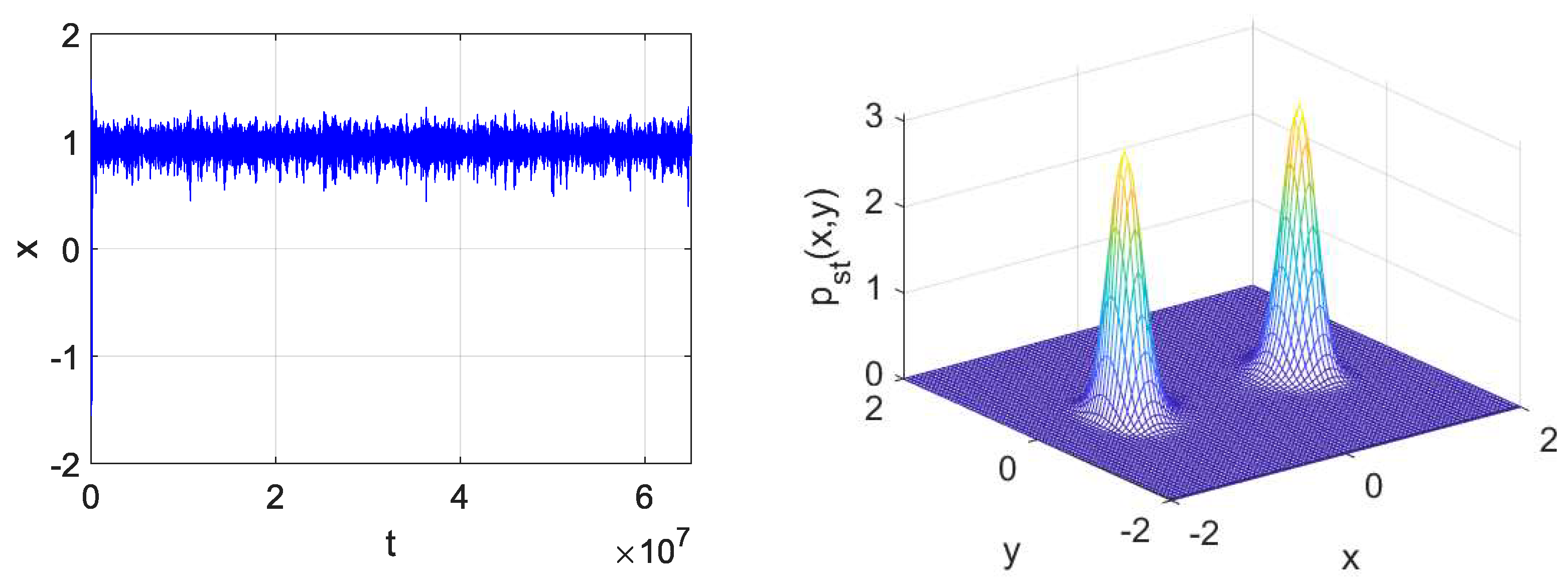
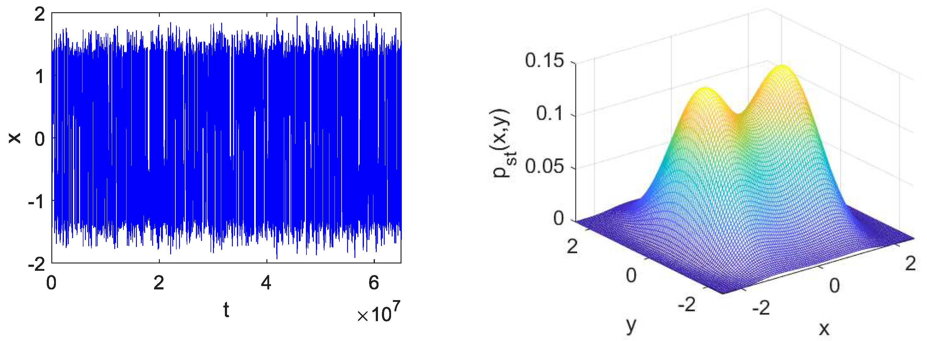
3.3. Stochastic Analysis: Averaging Techniques

Averaging techniques and perturbation methods are powerful techniques for the analysis of both deterministic and stochastic nonlinear dynamical systems. Therefore, it is not surprising that they have been applied to the analysis of energy harvesting systems [31,53,91,92].

3.3.1. Periodically Forced Nonlinear Oscillators and Averaging

Periodically forced nonlinear oscillators are a classical topic in nonlinear dynamics, perturbation methods and averaging techniques are particularly useful for their analysis [32,33]. For the sake of simplicity, let us consider a single-DOF system (Extension to systems with more DOFs is possible, but not straightforward, see for example [31].)

$$\ddot{x}+{\omega }_0^{2}x=\epsilon (Acos\left(\omega t\right)-\delta \dot{x}-\gamma x^3)$$

(43)

that can be interpreted as the (nonlinear) model for the mechanical part of an energy harvester, where the influence of the electro-mechanical coupling is negligible. Let us introduce the invertible coordinate transformation (Variable v used here should not be confused with a voltage.)

$$\left[\begin{array}{c}u\\ v\end{array}\right]=\left[\begin{array}{cc}cos\left(\omega t\right)& -{\displaystyle \frac{1}{\omega }}sin\left(\omega t\right)\\ -sin\left(\omega t\right)& -{\displaystyle \frac{1}{\omega }}cos\left(\omega t\right)\end{array}\right]\left[\begin{array}{c}x\\ \dot{x}\end{array}\right]$$

(44)

In the rotating reference frame, the unforced system is stationary. Taking the time derivatives gives

$$\begin{array}{cc}\hfill \dot{u}=& -{\displaystyle \frac{1}{\omega }}\left(\ddot{x}+{\omega }^{2}x\right)sin\left(\omega t\right)\hfill \end{array}$$

(45a)

$$\begin{array}{cc}\hfill \dot{v}=& -{\displaystyle \frac{1}{\omega }}\left(\ddot{x}+{\omega }^{2}x\right)cos\left(\omega t\right)\hfill \end{array}$$

(45b)

Introducing the frequency mismatch $\Omega =({\omega }_0^2-{\omega }^2)/\epsilon$, and using (43) yields

$$\begin{array}{cc}\hfill \dot{u}& =-{\displaystyle \frac{\epsilon }{\omega }}\left(Acos\left(\omega t\right)-\delta \dot{x}-\gamma x^3-\Omega x\right)sin\left(\omega t\right)\hfill \end{array}$$

(46a)

$$\begin{array}{cc}\hfill \dot{v}& =-{\displaystyle \frac{\epsilon }{\omega }}\left(Acos\left(\omega t\right)-\delta \dot{x}-\gamma x^3-\Omega x\right)cos\left(\omega t\right)\hfill \end{array}$$

(46b)

Inverting (44) and substituting into (46), gives a system of non autonomous ordinary differential equations for the unknown functions u and v. For small values of $\epsilon$, these equations can be averaged, integrating the right hand sides from 0 to $T=2\pi /\omega$ while holding u and v constant. With some abuse of notation, the same symbols shall be used to denote the averaged quantities. The following autonomous system is obtained:

$$\begin{array}{cc}\hfill \dot{u}& =-{\displaystyle \frac{\epsilon }{2\omega }}\left(\delta \omega u+{\displaystyle \frac{3}{4}}\gamma (u^2+v^2)v+\Omega v\right)\hfill \end{array}$$

(47a)

$$\begin{array}{cc}\hfill \dot{v}& =-{\displaystyle \frac{\epsilon }{2\omega }}\left(A+\delta \omega v-{\displaystyle \frac{3}{4}}\gamma (u^2+v^2)u-\Omega u\right)\hfill \end{array}$$

(47b)

Introducing the polar coordinates

$$r=\sqrt{u^2+v^2}\phi =arctan{\displaystyle \frac{u}{v}}$$

(48)

it is straightforward finding the differential equations

$$\begin{array}{cc}\hfill \dot{r}& =-{\displaystyle \frac{\epsilon }{2\omega }}\left(Asin\phi +\delta \omega r\right)\hfill \end{array}$$

(49a)

$$\begin{array}{cc}\hfill \dot{\phi }& ={\displaystyle \frac{\epsilon }{2\omega }}\left(\Omega +{\displaystyle \frac{3}{4}}\gamma r^2-{\displaystyle \frac{A}{r}}cos\phi \right)\hfill \end{array}$$

(49b)

The equilibrium points $(\overline{r},\overline{\phi })$ of (49) correspond to the limit cycles of (43). Setting the left hand sides equal to zero, squaring and summing, it is found that the equilibrium points are among the roots of the polynomial

$$p\left(r\right)={\displaystyle \frac{9}{16}}{\gamma }^2{r}^6+{\displaystyle \frac{3}{2}}\gamma \Omega r^4+\left({\Omega }^2+{\delta }^2{\omega }^2\right)r^2-A^2$$

(50)

The stability of the limit cycles is determined calculating the eigenvalues of the Jacobian matrix

$$J={\displaystyle \frac{\epsilon }{2\omega }}\left(\begin{array}{cc}-\delta \omega & -\Omega \overline{r}-3\gamma {\overline{r}}^3/4\\ 9\gamma \overline{r}/4+\Omega /\overline{r}& -\delta \omega \end{array}\right)$$

(51)

The blue and red lines in Figure 8, show the typical frequency response for a nonlinear oscillator. Consider the case of a stiffening elastic beam (on the left). For the case of a softening beam, the behaviour as the frequency is varied is simply reversed. For small values of the forcing frequency, the nonlinear oscillator exhibits a unique stable periodic solution, whose amplitude increases as the forcing frequency is increased. At the critical value ${\omega }_{S{N}_1}$, a saddle node of limit cycles bifurcation occurs. Two new periodic solutions emerge, one is asymptotically stable, while the other is unstable of saddle type. Increasing the frequency further the two, initially coincident limit cycles, separate. At the second critical value ${\omega }_{S{N}_2}$, the unstable limit cycle collides with the original stable one, and the two solutions vanish through a second limit cycle saddle node bifurcation. For $\omega >{\omega }_{S{N}_2}$, the small amplitude stable limit cycle remains the unique periodic solution. The amplitude response of a linear oscillator is also shown for reference (black line) in Figure 8. With respect to its linear counterpart, the nonlinear oscillator offers a lower maximum oscillation amplitude, but, thanks to the hysteretic response, the amplitude is altogether higher on a wider frequency band.

3.3.2. Stochastic Averaging and Adiabatic Elimination

Stochastic averaging and adiabatic elimination are very powerful tools to obtain the stationary distribution for systems with time scale separation between variables [93,94,95,96,97,98,99]. Both methods rely on the fact that the fast variables quickly relax to a stationary distribution. As a matter of fact, they do so in such a short time that the slow variables do not change significantly. This property is then used to define a projection operator that reduces the dynamics to a sub-manifold, representing a system of averaged (or coarse grained) SDEs.

To illustrate the technique, consider the system of SDEs

$$\begin{array}{cc}\hfill d{\mathbf{X}}_t=& \mathbf{a}({\mathbf{X}}_t,Y_y)dt+\mathbf{B}({\mathbf{X}}_t,Y_t)d{W}_t\hfill \end{array}$$

(52a)

$$\begin{array}{cc}\hfill d{Y}_t=& \left({\displaystyle \frac{1}{{\epsilon }^2}}c\left(Y_t\right)+{\displaystyle \frac{1}{\epsilon }}d({\mathbf{X}}_t,Y_t)\right)dt+{\displaystyle \frac{1}{\epsilon }}D\left(Y_t\right)d{W}_t\hfill \end{array}$$

(52b)

where $\epsilon$ is a small parameter. For the sake of simplicity, a scalar fast variable $y\left(t\right)$ is considered. Let $u(\mathbf{x},y,t)=E\left[f\right(\mathbf{x},y,t\left)\right]$ denote the expectation of a generic function $f(\mathbf{x},y,t)$. The Forward Kolmogorov Equation (FKE) associated to (52) is [37]

$${\displaystyle \frac{\partial u(\mathbf{x},y,t)}{\partial t}}=\left({\Lambda }_0+{\displaystyle \frac{1}{\epsilon }}{\Lambda }_1+{\displaystyle \frac{1}{{\epsilon }^2}}{\Lambda }_2\right)u(\mathbf{x},y,t)$$

(53)

where the operators on the right-hand-side are defined as

$$\begin{array}{cc}\hfill {\Lambda }_{0}u=& \sum _{i=1}^N{a}_i(\mathbf{x},y,t){\displaystyle \frac{\partial u}{\partial x_i}}+{\displaystyle \frac{1}{2}}\sum _{i,j=1}^N{\left(\mathbf{B}(\mathbf{x},y){\mathbf{B}}^T(\mathbf{x},y)\right)}_{ij}{\displaystyle \frac{{\partial }^{2}u}{\partial x_i\partial x_j}}\hfill \end{array}$$

(54a)

$$\begin{array}{cc}\hfill {\Lambda }_{1}u=& d(\mathbf{x},y){\displaystyle \frac{\partial u}{\partial y}}\hfill \end{array}$$

(54b)

$$\begin{array}{cc}\hfill {\Lambda }_{2}u=& c\left(y\right){\displaystyle \frac{\partial u}{\partial y}}+{\displaystyle \frac{1}{2}}{D}^2\left(y\right){\displaystyle \frac{{\partial }^{2}u}{\partial y^2}}\hfill \end{array}$$

(54c)

For the solution of the FKE consider the ansatz $u(\mathbf{x},y,t)=u_0(\mathbf{x},y,t)+\epsilon u_1(\mathbf{x},y,t)+{\epsilon }^{2}u(\mathbf{x},y,t)+\dots$. Substituting the ansatz into (53) and equating the same powers of $\epsilon$ yields

$$\begin{array}{cc}\hfill {\epsilon }^{-2}:{\Lambda }_2{u}_0=& 0\hfill \end{array}$$

(55a)

$$\begin{array}{cc}\hfill {\epsilon }^{-1}:{\Lambda }_2{u}_1=& -{\Lambda }_1{u}_0\hfill \end{array}$$

(55b)

$$\begin{array}{cc}\hfill {\epsilon }^0:{\Lambda }_2{u}_2=& {\displaystyle \frac{\partial u_0}{\partial t}}-{\Lambda }_1{u}_1-{\Lambda }_0{u}_0\hfill \end{array}$$

(55c)

The first Equation (55a) of the hierarchy implies that $u_0$ does not depend on y, i.e., $u_0=u_0(\mathbf{x},t)$. The remaining two equations are of the type ${\Lambda }_2{u}_n=b_n$. Fredholm alternative theorem establishes that these equations are solvable, provided that a function $\psi$ exists such that $\psi \in \ker \left({\Lambda }_2^{*}\right)$, where ${\Lambda }_2^{*}$ is the conjugate operator and $\ker$ denotes the kernel, and that each $b_n$ is orthogonal to $\ker \left({\Lambda }_2^{*}\right)$. Taking into account (54c), ${\Lambda }_2^{*}\psi =0$ implies that $\psi$ is the stationary distribution for the lowest order approximation of the fast dynamics, e.g., $\psi ={\rho }_{st}\left(y\right)$. Being orthogonal to $\ker \left({\Lambda }_2^{*}\right)$ means that $(b_n,\psi )=0$, where $(·,·)$ denotes the inner product in the $L_2$ Banach space. As a consequence, the orthogonality condition implies that each term $b_n$ averages to zero with respect to y

$$(b_n,\psi )={\int }_{\mathbb{R}}{b}_n{\rho }_{st}\left(y\right)dy=E{\left[b_n\right]}_y$$

(56)

where $E{\left[b_n\right]}_y$ denotes expectation with respect to y. Since $u_0$ is independent of y, (55b) is solvable, with

$$u_1(\mathbf{x},y,t)=-{\Lambda }_2^{-1}{\Lambda }_1{u}_0(\mathbf{x},t)$$

(57)

Similarly, (55c) is solvable provided that

$${\displaystyle \frac{\partial u_0(\mathbf{x},t)}{\partial t}}=E{\left[{\Lambda }_0\right]}_y{u}_0(\mathbf{x},t)-E{\left[{\Lambda }_1{\Lambda }_2^{-1}{\Lambda }_1\right]}_y{u}_0(\mathbf{x},t)$$

(58)

that corresponds to the FKE associated to a reduced SDE applying to the slow variables $\mathbf{x}$ only.

As an example, consider again a single-DOF model

$$\begin{array}{cc}\hfill dx=& ydt\hfill \end{array}$$

(59a)

$$\begin{array}{cc}\hfill dy=& \left(-U^{\prime }\left(x\right)-\rho y\right)dt+\epsilon d{W}_t\hfill \end{array}$$

(59b)

In the absence of friction and noise (for $\rho =\epsilon =0$), the underlying system is Hamiltonian. The governing equations can be rewritten in terms of the energy $E=\frac{1}{2}{y}^2+U\left(x\right)$ and the angle $\theta (x,y)$ (The explicit expression for the angle $\theta$ depends on the specific form of the potential $U\left(x\right)$.) obtaining [92]

$$\begin{array}{cc}\hfill dE=& \left(-\rho y^2(E,\theta )+{\displaystyle \frac{{\epsilon }^2}{2}}\right)dt+\epsilon y(E,\theta )d{W}_t\hfill \end{array}$$

(60a)

$$\begin{array}{cc}\hfill d\theta =& \left(\Omega \left(E\right)-\rho y(E,\theta ){\displaystyle \frac{\partial \theta }{\partial y}}+{\displaystyle \frac{{\epsilon }^2}{2}}{\displaystyle \frac{{\partial }^2\theta }{\partial y^2}}\right)dt+\epsilon {\displaystyle \frac{\partial \theta }{\partial y}}d{W}_t\hfill \end{array}$$

(60b)

where $\Omega \left(E\right)=\frac{\partial \theta }{\partial x}y-\frac{\partial \theta }{\partial y}{U}^{\prime }\left(x\right)$ is the energy dependent frequency of the underlying Hamiltonian systems. Introducing the scaled time $\tau =t/{\epsilon }^2$ and using the time change theorem for SDEs [37], the energy and the angle have the same distributions as the solutions of the SDEs

$$\begin{array}{cc}\hfill dE=& \left(-{\displaystyle \frac{\rho }{{\epsilon }^2}}y(E,\theta )+{\displaystyle \frac{1}{2}}\right)dt+y(E,\theta )d{W}_t\hfill \end{array}$$

(61a)

$$\begin{array}{cc}\hfill d\theta =& \left({\displaystyle \frac{1}{{\epsilon }^2}}\Omega \left(E\right)-{\displaystyle \frac{\rho }{{\epsilon }^2}}y(E,\theta ){\displaystyle \frac{\partial \theta }{\partial y}}+{\displaystyle \frac{1}{2}}{\displaystyle \frac{{\partial }^2\theta }{\partial y^2}}\right)dt+{\displaystyle \frac{\partial \theta }{\partial y}}d{W}_t\hfill \end{array}$$

(61b)

Assuming $\rho ={\epsilon }^2$ for simplicity, the operators of the FKE take the form:

$$\begin{array}{cc}\hfill {\Lambda }_2{u}_0=& \Omega \left(E\right){\displaystyle \frac{\partial u_0}{\partial \theta }}\hfill \end{array}$$

(62a)

$$\begin{array}{cc}\hfill {\Lambda }_0{u}_0=& \left(-y+{\displaystyle \frac{1}{2}}\right){\displaystyle \frac{\partial u_0}{\partial E}}+\left(y{\displaystyle \frac{\partial \theta }{\partial y}}+{\displaystyle \frac{1}{2}}{\displaystyle \frac{{\partial }^2\theta }{\partial y^2}}\right){\displaystyle \frac{\partial u_0}{\partial \theta }}+{\displaystyle \frac{1}{2}}{y}^2{\displaystyle \frac{{\partial }^2{u}_0}{\partial E^2}}+{\displaystyle \frac{1}{2}}{\left({\displaystyle \frac{\partial \theta }{\partial y}}\right)}^2{\displaystyle \frac{{\partial }^2{u}_0}{\partial {\theta }^2}}\hfill \end{array}$$

(62b)

Equation (62a) implies that the lowest order stationary distribution is independent of the angle, ${\widehat{p}}_{st}={\widehat{p}}_{st}\left(E\right)$. Imposing the normalization condition ${\int }_0^{2\pi }{\widehat{p}}_{st}\left(E\right)d\theta =1$ yields ${\widehat{p}}_{st}={\left(2\pi \right)}^{-1}$. This stationary distribution is used to average with respect to the fast angle variable. Imposing periodic boundary conditions, a scalar averaged SDE for the energy is obtained

$$dE=\left(-\overline{y^2}\left(E\right)+{\displaystyle \frac{1}{2}}\right)dt+\overline{y}\left(E\right)d{W}_t$$

(63)

where

$$\begin{array}{cc}\hfill \overline{y^2}\left(E\right)=& {\displaystyle \frac{1}{2\pi }}{\int }_0^{2\pi }{y}^2(E,\theta )d\theta \hfill \end{array}$$

(64a)

$$\begin{array}{cc}\hfill \overline{y}\left(E\right)=& {\displaystyle \frac{1}{2\pi }}{\int }_0^{2\pi }y(E,\theta )d\theta \hfill \end{array}$$

(64b)

A stationary solution for the reduced order Fokker–Planck equation associated to (63) can be easily found, and the solution can be used to calculate the relevant expected quantities [92].

3.4. Numerical Analysis Methods

Numerical methods are often the unique way to obtain detailed information about nonlinear dynamical systems, and, in particular, for the case of stochastic excitations. There are many excellent references about numerical methods for stochastic differential equations [100,101,102,103,104,105]. This section provides an overview of the main numerical techniques, based on [106].

Numerical schemes for ODEs are recalled first. For the sake of simplicity, let us consider the autonomous ODE system (Any non-autonomous system can be transformed into autonomous, rewriting the time as an additional “puppet” variable, and increasing the number of variables by one.)

$${\displaystyle \frac{d\mathbf{x}\left(t\right)}{dt}}=\mathbf{f}\left(\mathbf{x}\left(t\right)\right)$$

(65)

Expanding $\mathbf{x}\left(t\right)$ in Taylor series

$$\begin{array}{cc}\hfill \mathbf{x}\left(t\right)& =\mathbf{x}\left(t_0\right)+{\displaystyle \frac{d\mathbf{x}\left(t_0\right)}{dt}}(t-t_0)+{\displaystyle \frac{1}{2!}}{\displaystyle \frac{d^2\mathbf{x}\left(t_0\right)}{d{t}^2}}{(t-t_0)}^2+\dots \hfill \\ \hfill & =\mathbf{x}\left(t_0\right)+\mathbf{f}\left(\mathbf{x}\left(t_0\right)\right)(t-t_0)+{\displaystyle \frac{1}{2!}}{\displaystyle \frac{\partial \mathbf{f}\left(\mathbf{x}\left(t_0\right)\right)}{\partial \mathbf{x}}}\mathbf{f}\left(\mathbf{x}\left(t_0\right)\right){(t-t_0)}^2+\dots \hfill \end{array}$$

(66)

Setting $t=t_0+\Delta t$ and truncating the Taylor expansion to quadratic terms yields:

$$\mathbf{x}(t_0+\Delta t)=\mathbf{x}\left(t_0\right)+\mathbf{f}\left(\mathbf{x}\left(t_0\right)\right)\Delta t+{\displaystyle \frac{1}{2}}{\displaystyle \frac{\partial \mathbf{f}\left(\mathbf{x}\left(t_0\right)\right)}{\partial \mathbf{x}}}\mathbf{f}\left(\mathbf{x}\left(t_0\right)\right)\Delta t^2$$

(67)

To avoid the explicit calculation of the Jacobian matrix $\partial \mathbf{f}\left(\mathbf{x}\left(t_0\right)\right)/\partial \mathbf{x}$, one can try the form

$$\mathbf{x}(t_0+\Delta t)=\mathbf{x}\left(t_0\right)+a\mathbf{f}\left(\mathbf{x}\left(t_0\right)\right)\Delta t+b\mathbf{f}\left(\mathbf{x}\left(t_0\right)+c\mathbf{f}\left(\mathbf{x}\left(t_0\right)\right)\Delta t\right)\Delta t$$

(68)

where a, b and c are constant to be determined, and the following approximation is made

$$\mathbf{f}\left(\mathbf{x}\left(t_0\right)+c\mathbf{f}\left(\mathbf{x}\left(t_0\right)\right)\Delta t\right)\approx \mathbf{f}\left(\mathbf{x}\left(t_0\right)\right)+{\displaystyle \frac{\partial \mathbf{f}\left(\mathbf{x}\left(t_0\right)\right)}{\partial \mathbf{x}}}\mathbf{f}(\mathbf{x}\left(t_0\right)\Delta t$$

(69)

Comparing (67), (68) and (69), it is found that $a+b=1$ and $bc=1/2$. Thus the solution to (65) can be approximated as

$$\check{\mathbf{x}}(t_0+\Delta t)=\mathbf{x}\left(t_0\right)+{\displaystyle \frac{1}{2}}\mathbf{f}({\tilde{\mathbf{x}}}_1+\mathbf{f}\left({\tilde{\mathbf{x}}}_2\right))\Delta t$$

(70)

where ${\tilde{\mathbf{x}}}_1=\mathbf{x}\left(t_0\right)$ and ${\tilde{\mathbf{x}}}_2=\mathbf{x}\left(t_0\right)+\mathbf{f}\left({\tilde{\mathbf{x}}}_1\right)\Delta t$.

This algorithm is a two-stage method. Higher-order methods becomeincreasingly complex with the number of terms. They are constructed evaluating the function $\mathbf{f}\left(\mathbf{x}\right(t\left)\right)$ at a number of points and weighting the terms. The Runge–Kutta method gives the following approximation for the solution $\mathbf{x}\left(t\right)$ in the time interval $t_0<t_1<\dots <t_N=t$:

$$\begin{array}{cc}\hfill \check{\mathbf{x}}\left(t_{k+1}\right)=& \check{\mathbf{x}}\left(t_k\right)+\sum _{i=1}^s{\alpha }_i\mathbf{f}\left({\tilde{\mathbf{x}}}_i\right)\Delta t\hfill \end{array}$$

(71)

$$\begin{array}{cc}\hfill {\tilde{\mathbf{x}}}_i=& \check{\mathbf{x}}\left(t_k\right)+\sum _{j=1}^{i-1}{A}_{ij}\mathbf{f}\left({\tilde{\mathbf{x}}}_j\right)\Delta t\hfill \end{array}$$

(72)

where the coefficients ${\alpha }_i$ and $A_{ij}$ are given by the Butcher tableau [106]. At the lowest order, the Runge–Kutta method gives the common forward Euler method

$$\check{\mathbf{x}}\left(t_{k+1}\right)=\check{\mathbf{x}}\left(t_k\right)+\mathbf{f}\left(\check{\mathbf{x}}\left(t_k\right)\right)\Delta t$$

(73)

The classic fourth order Runge–Kutta method gives the approximation

$$\begin{array}{cc}\hfill \check{\mathbf{x}}\left(t_{k+1}\right)=& \check{\mathbf{x}}\left(t_k\right)+{\displaystyle \frac{1}{6}}\left(\mathbf{f}\left({\tilde{\mathbf{x}}}_1\right)+2\mathbf{f}\left({\tilde{\mathbf{x}}}_2\right)+2\mathbf{f}\left({\tilde{\mathbf{x}}}_3\right)+\mathbf{f}\left({\tilde{\mathbf{x}}}_4\right)\right)\Delta t\hfill \end{array}$$

(74a)

$$\begin{array}{cc}\hfill {\tilde{\mathbf{x}}}_1=& \check{\mathbf{x}}\left(t_k\right)\hfill \end{array}$$

(74b)

$$\begin{array}{cc}\hfill {\tilde{\mathbf{x}}}_2=& \check{\mathbf{x}}\left(t_k\right)+{\displaystyle \frac{1}{2}}\mathbf{f}\left({\tilde{\mathbf{x}}}_1\right)\Delta t\hfill \end{array}$$

(74c)

$$\begin{array}{cc}\hfill {\tilde{\mathbf{x}}}_3=& \check{\mathbf{x}}\left(t_k\right)+{\displaystyle \frac{1}{2}}\mathbf{f}\left({\tilde{\mathbf{x}}}_2\right)\Delta t\hfill \end{array}$$

(74d)

$$\begin{array}{cc}\hfill {\tilde{\mathbf{x}}}_4=& \check{\mathbf{x}}\left(t_k\right)+\mathbf{f}\left({\tilde{\mathbf{x}}}_3\right)\Delta t\hfill \end{array}$$

(74e)

The methods above can be generalized to SDEs, replacing the Taylor series for ODEs with the Itô-Taylor development in the stochastic case. The derivation is basically the same, and thus it is not repeated here, except for the fact that time derivative computations are replaced by applications of the Itô formula. The interested reader is referred to [106] for details. As before, the discussion is limited to the autonomous case. Consider the SDEs

$$d\mathbf{X}\left(t\right)=\mathbf{f}\left(\mathbf{X}\right(t\left)\right)dt+\mathbf{L}\left(\mathbf{X}\right(t\left)\right)d\mathbf{W}\left(t\right)$$

(75)

where $\mathbf{f}\left(\mathbf{X}\right(t\left)\right)$ is the drift vector, $\mathbf{L}\left(\mathbf{X}\right(t\left)\right)$ is the diffusion matrix, and $\mathbf{W}\left(t\right)$ is a vector of Wiener processes. Repeating the previous procedure, replacing Taylor with Itô-Taylor series, leads to the form

$$\mathbf{X}\left(t\right)=\mathbf{X}\left(t_0\right)+\mathbf{f}\left(\mathbf{X}\left(t_0\right)\right)\Delta t+\mathbf{L}\left(\mathbf{X}\left(t_0\right)\right)(\mathbf{W}\left(t\right)-\mathbf{W}\left(t_0\right))+\mathbf{R}\left(t\right)$$

(76)

where $\mathbf{R}\left(t\right)$ is a remainder consisting of higher-order multiple stochastic integrals involving drift, diffusion, and their derivatives. Neglecting the remainder gives the simple Euler–Maruyama (EM) algorithm, that represents the direct extension of the Euler method to SDEs

$$\check{\mathbf{X}}\left(t_{k+1}\right)=\check{\mathbf{X}}\left(t_k\right)+\mathbf{f}\left(\check{\mathbf{X}}\left(t_k\right)\right)\Delta t+\mathbf{L}\left(\check{\mathbf{X}}\left(t_k\right)\right)(\mathbf{W}\left(t_{k+1}\right)-\mathbf{W}\left(t_k\right))$$

(77)

In fact, the EM method reduces to the Euler method for $\mathbf{L}\left(\mathbf{X}\right(t\left)\right)=0$.

As a matter of fact, the EM solution matches the true solution more closely as $\Delta t$ is decreased. A numerical integration method is said to have strong order of convergence equal to $\gamma$ if a constant K exists such that

$$E\left[\right|\mathbf{X}\left(t_M\right)-\check{\mathbf{X}}\left(t_M\right)\left|\right]\le K\Delta t^{\gamma }$$

(78)

for any fixed $t_M=m\Delta t\in [0,T]$ and $\Delta t$ sufficiently small. The strong order of convergence measures the decay rate of the “mean of the error” decays as $\Delta t\to 0$ [101]. A less demanding alternative is to measure the rate of decay of the “error of the means”, namely, the order of weak convergence. A method is said to have weak order of convergence equal to $\gamma$ if there exists a constant K such that for all functions p in some class

$$|E\left[p\left(\mathbf{X}\left(t_M\right)\right)\right]-E\left[p\left(\check{\mathbf{X}}\left(t_M\right)\right)\right]|\le K\Delta t^{\gamma }$$

(79)

for any fixed $t_M=m\Delta t\in [0,T]$ and $\Delta t$ sufficiently small [101]. The EM method has strong order of convergence $\gamma =1/2$ and weak order of convergence $\gamma =1$ [103].

Taking into account additional terms in the remainder, leads to higher order methods, such as the Milstein method. The Milstein method gives the following approximation for the solution:

$$\begin{array}{cc}\hfill \check{\mathbf{X}}\left(t_{k+1}\right)=& \check{\mathbf{X}}\left(t_k\right)+\mathbf{f}\left(\check{\mathbf{X}}\left(t_k\right)\right)\Delta t+\mathbf{L}\left(\check{\mathbf{X}}\left(t_k\right)\right)(\mathbf{W}\left(t_{k+1}\right)-\mathbf{W}\left(t_k\right))\hfill \\ \hfill & +\sum _j\left[\sum _i{\displaystyle \frac{\partial \mathbf{L}\left(\check{\mathbf{X}}\left(t_k\right)\right)}{\partial X_i}}{\mathbf{L}}_{ij}\left(\check{\mathbf{X}}\left(t_k\right)\right)\right]\Delta {\chi }_{jk}\hfill \end{array}$$

(80)

where

$$\Delta {\chi }_{jk}={\int }_{t_k}^{t_{k+1}}{\int }_{t_k}^{\tau }d{W}_j\left(\tau \right)d\mathbf{W}\left(\tau \right)$$

(81)

The two main limitations in the application of the Milstein method are: (1) it requires the explicit calculation of the derivatives of the diffusion matrix; (2) the solution of the iterated integrals (81) is required. For additive noise, the diffusion matrix is constant $\mathbf{L}\left(\mathbf{x}\right(t\left)\right)=\mathbf{L}$, the derivatives of the diffusion matrix are null and the Milstein method coincides with the EM method. For the iterated integral, a significant simplification is obtained in the scalar case, where

$$\Delta {\chi }_k={\int }_{t_k}^{t_{k+1}}{\int }_{t_k}^{\tau }dW\left(\tau \right)dW\left(\tau \right)={\displaystyle \frac{1}{2}}{\left(W\left(t_{k+1}\right)-W\left(t_k\right)\right)}^2-\Delta t$$

(82)

To avoid calculating the derivatives of the diffusion matrix, discrete time approximation may be used, leading to stochastic Runge-Kutta methods. The EM scheme can be seen as the simplest stochastic Runge–Kutta method, in the same way as the Euler method can be seen as the simplest Runge–Kutta scheme for ODEs. The higher-order stochastic Runge–Kutta method can be derived replacing the derivatives in the Milstein method with suitable finite differences. Unfortunately, the iterated Itô integrals occurring in the remainder cannot be eliminated so easily, and stochastic versions of Runge–Kutta methods cannot be derived as trivial extensions of the Runge–Kutta method for ODEs [107]. Similarly to the case for ODEs, the stochastic Runge–Kutta method with strong order 1 convergence can be formulated, where iterated integrals are avoided in the scheme and only appear in the supporting values [105]. The resulting approximation is

$$\begin{array}{cc}\hfill \check{\mathbf{X}}\left(t_{k+1}\right)=& \check{\mathbf{X}}\left(t_k\right)+{\displaystyle \frac{1}{2}}\left(\mathbf{f}(\check{\mathbf{X}}\left(t_k\right)+\mathbf{f}\left({\tilde{\mathbf{X}}}_2^{\left(0\right)}\right)\right)\Delta t\hfill \\ \hfill & +\sum _n\left({\mathbf{L}}_n\left(\check{\mathbf{X}}\left(t_k\right)\right)\Delta W_k^{\left(n\right)}+{\displaystyle \frac{\sqrt{\Delta t}}{2}}\left({\mathbf{L}}_n\left({\tilde{\mathbf{X}}}_2^{\left(n\right)}\right)-{\mathbf{L}}_n\left({\tilde{\mathbf{X}}}_3^{\left(n\right)}\right)\right)\right)\hfill \end{array}$$

(83)

where $\Delta W_k^{\left(n\right)}=W^{\left(n\right)}\left(t_{k+1}\right)-W^{\left(n\right)}\left(t_k\right)$, and the supporting values are

$$\begin{array}{cc}\hfill {\tilde{\mathbf{X}}}_2^{\left(0\right)}=& \mathbf{X}\left(t_k\right)+\mathbf{f}\left(\mathbf{X}\left(t_k\right)\right)\Delta t\hfill \end{array}$$

(84a)

$$\begin{array}{cc}\hfill {\tilde{\mathbf{X}}}_2^{\left(n\right)}=& \mathbf{X}\left(t_k\right)+\mathbf{f}\left(\mathbf{X}\left(t_k\right)\right)\Delta t+\sum _n{\mathbf{L}}_n\left(\mathbf{X}\left(t_k\right)\right){\displaystyle \frac{\Delta {\chi }_k^{(l,n)}}{\sqrt{\Delta t}}}\hfill \end{array}$$

(84b)

$$\begin{array}{cc}\hfill {\tilde{\mathbf{X}}}_3^{\left(n\right)}=& \mathbf{X}\left(t_k\right)+\mathbf{f}\left(\mathbf{X}\left(t_k\right)\right)\Delta t-\sum _n{\mathbf{L}}_n\left(\mathbf{X}\left(t_k\right)\right){\displaystyle \frac{\Delta {\chi }_k^{(l,n)}}{\sqrt{\Delta t}}}\hfill \end{array}$$

(84c)

and

$$\Delta {\chi }_k^{(l,n)}={\int }_{t_k}^{t_{k+1}}{\int }_{t_k}^{{\tau }_2}d{W}_l\left({\tau }_1\right)d{W}_n\left({\tau }_2\right)$$

(85)

When $l=n$ the multiple Itô integrals can be rewritten as

$$\Delta {\chi }_k^{(n,n)}={\displaystyle \frac{1}{2}}\left({\left(\Delta W_k^{\left(n\right)}\right)}^2-\Delta t\right)$$

(86)

To derive higher-order methods, more terms in the Itô–Taylor expansion must be considered, but the problem becomes rapidly impractical because of the number of functions that must be evaluated and their complexity. In some special cases, such as systems with symmetry or for additive noise, higher order methods are still feasible. Otherwise, methods of higher order weak convergence should be considered, instead.

4. Conclusions

This paper presented a review on the modeling and analysis of energy harvesters collecting mechanical energy in the form of vibrations, taking a different perspective with respect to most other contributions. In fact, the focus is on the modeling techniques that apply to the entire energy source/mechanical oscillator/transducer/electrical load chain, pointing out how mechanical–electrical analogies can be effectively exploited to represent the collective behaviour as the cascade of equivalent electrical two-ports. This representation, particularly effective in the case of linear elements, is the natural environment in which enhancing the efficiency of the collected energy transfer to the load, by means of the interposition of a properly designed matching network, can be introduced.

On the other hand, two other main issues are taken into account in this review: the presence, intentional or deliberate, of nonlinearities in the mechanical part modeling or in the transducer description, and the advanced analysis techniques required for a proper description of the harvester, both analytical (or semi-analytical) and numerical. In the frequency domain, the powerful numerical harmonic balance technique was discussed, after introducing the basic concepts in the linear case. In the time domain, after introducing deterministic and stochastic averaging approaches, several numerical techniques well suited for the analysis of nonlinear harvesting systems in the presence of deterministic or random mechanical vibrations were discussed.

The main conclusion is, therefore, that the fast growing development of energy harvesting techniques has now reached a maturity level which permits leaving the starting, although unavoidable, pre-requisite level of the purely technological development of the mechanical energy collection system and of the transducer realization, to enter the stage of collective design and optimization of the energy transfer to the load. This step can definitely benefit from the exploitation of consolidated techniques available from other fields, ranging from advanced mathematical description and treatment of the system, to the interposition of matching networks enhancing the power transfer.

References

1. Misra, S.; Mukherjee, A.; Roy, A. Introduction to IoT; University of Cambridge ESOL Examinations: Cambridge, UK, 2021. [Google Scholar]
2. IoT 2022: Connected Devices Growing 18% to 14.4 Billion Globally. Available online: https://www.iotforall.com/state-of-iot-2022 (accessed on 22 February 2023).
3. Munoz-Ausecha, C.; Ruiz-Rosero, J.; Ramirez-Gonzalez, G. RFID Applications and Security Review. Computation 2021, 9, 69. [Google Scholar] [CrossRef]
4. Penella-López, M.T.; Gasulla-Forner, M. Powering Autonomous Sensors An Integral Approach with Focus on Solar and RF Energy Harvesting; Springer London, Limited: London, UK, 2011. [Google Scholar]
5. Roundy, S.; Wright, P.K.; Rabaey, J.M. Energy Scavenging for Wireless Sensor Networks; Springer: New York, NY, USA, 2003. [Google Scholar]
6. Paradiso, J.A.; Starner, T. Energy scavenging for mobile and wireless electronics. IEEE Pervasive Comput. 2005, 4, 18–27. [Google Scholar] [CrossRef]
7. Beeby, S.P.; Tudor, M.J.; White, N.M. Energy harvesting vibration sources for microsystems applications. Meas. Sci. Technol. 2006, 17, R175. [Google Scholar] [CrossRef]
8. Mitcheson, P.; Yeatman, E.; Rao, G.; Holmes, A.; Green, T. Energy Harvesting From Human and Machine Motion for Wireless Electronic Devices. Proc. IEEE 2008, 96, 1457–1486. [Google Scholar] [CrossRef]
9. Lu, X.; Wang, P.; Niyato, D.; Kim, D.I.; Han, Z. Wireless Networks with RF Energy Harvesting: A Contemporary Survey. IEEE Commun. Surv. Tutor. 2015, 17, 757–789. [Google Scholar] [CrossRef]
10. Akinaga, H. Recent advances and future prospects in energy harvesting technologies. Jpn. J. Appl. Phys. 2020, 59, 110201. [Google Scholar] [CrossRef]
11. Anton, S.R.; Sodano, H.A. A review of power harvesting using piezoelectric materials (2003–2006). Smart Mater. Struct. 2007, 16, R1. [Google Scholar] [CrossRef]
12. Priya, S.; Inman, D.J. Energy Harvesting Technologies; Springer: New York, NY, USA, 2009; Volume 21. [Google Scholar]
13. Liu, H.; Zhong, J.; Lee, C.; Lee, S.W.; Lin, L. A comprehensive review on piezoelectric energy harvesting technology: Materials, mechanisms, and applications. Appl. Phys. Rev. 2018, 5, 041306. [Google Scholar] [CrossRef]
14. Covaci, C.; Gontean, A. Piezoelectric energy harvesting solutions: A review. Sensors 2020, 20, 3512. [Google Scholar] [CrossRef]
15. Tang, L.; Yang, Y.; Soh, C.K. Toward broadband vibration-based energy harvesting. J. Intell. Mater. Syst. Struct. 2010, 21, 1867–1897. [Google Scholar] [CrossRef]
16. Khaligh, A.; Zeng, P.; Zheng, C. Kinetic energy harvesting using piezoelectric and electromagnetic technologies–state of the art. IEEE Trans. Ind. Electron. 2009, 57, 850–860. [Google Scholar] [CrossRef]
17. Wei, C.; Jing, X. A comprehensive review on vibration energy harvesting: Modelling and realization. Renew. Sustain. Energy Rev. 2017, 74, 1–18. [Google Scholar] [CrossRef]
18. Iqbal, M.; Nauman, M.M.; Khan, F.U.; Abas, P.E.; Cheok, Q.; Iqbal, A.; Aissa, B. Vibration-based piezoelectric, electromagnetic, and hybrid energy harvesters for microsystems applications: A contributed review. Int. J. Energy Res. 2021, 45, 65–102. [Google Scholar] [CrossRef]
19. Gammaitoni, L.; Neri, I.; Vocca, H. The benefits of noise and nonlinearity: Extracting energy from random vibrations. Chem. Phys. 2010, 375, 435–438. [Google Scholar] [CrossRef]
20. Gammaitoni, L. There’s plenty of energy at the bottom (micro and nano scale nonlinear noise harvesting). Contemp. Phys. 2012, 53, 119–135. [Google Scholar] [CrossRef]
21. Daqaq, M.F.; Masana, R.; Erturk, A.; Dane Quinn, D. On the role of nonlinearities in vibratory energy harvesting: A critical review and discussion. Appl. Mech. Rev. 2014, 66. [Google Scholar] [CrossRef]
22. Hannan, M.A.; Mutashar, S.; Samad, S.A.; Hussain, A. Energy harvesting for the implantable biomedical devices: Issues and challenges. Biomed. Eng. Online 2014, 13, 1–23. [Google Scholar] [CrossRef]
23. Yildirim, T.; Ghayesh, M.H.; Li, W.; Alici, G. A review on performance enhancement techniques for ambient vibration energy harvesters. Renew. Sustain. Energy Rev. 2017, 71, 435–449. [Google Scholar] [CrossRef]
24. Tran, N.; Ghayesh, M.H.; Arjomandi, M. Ambient vibration energy harvesters: A review on nonlinear techniques for performance enhancement. Int. J. Eng. Sci. 2018, 127, 162–185. [Google Scholar] [CrossRef]
25. Nguyen, V.T.; Kumar, P.; Leong, J. Finite Element Modelling and Simulations of Piezoelectric Actuators Responses with Uncertainty Quantification. Computation 2018, 6, 60. [Google Scholar] [CrossRef]
26. Khazaee, M.; Rezania, A.; Rosendahl, L. Piezoelectric resonator design and analysis from stochastic car vibration using an experimentally validated finite element with viscous-structural damping model. Sustain. Energy Technol. Assess. 2022, 52, 102228. [Google Scholar] [CrossRef]
27. Khazaee, M.; Huber, J.E.; Rosendahl, L.; Rezania, A. Four-point bending piezoelectric energy harvester with uniform surface strain toward better energy conversion performance and material usage. J. Sound Vib. 2023, 548, 117492. [Google Scholar] [CrossRef]
28. Erturk, A.; Hoffmann, J.; Inman, D.J. A piezomagnetoelastic structure for broadband vibration energy harvesting. Appl. Phys. Lett. 2009, 94, 254102. [Google Scholar] [CrossRef]
29. Erturk, A.; Inman, D.J. Piezoelectric Energy Harvesting; John Wiley & Sons: Chichester, UK, 2011. [Google Scholar]
30. Harne, R.L.; Thota, M.; Wang, K.W. Concise and high-fidelity predictive criteria for maximizing performance and robustness of bistable energy harvesters. Appl. Phys. Lett. 2013, 102, 053903. [Google Scholar] [CrossRef]
31. Bonnin, M.; Traversa, F.L.; Bonani, F. Leveraging circuit theory and nonlinear dynamics for the efficiency improvement of energy harvesting. Nonlinear Dyn. 2021, 104, 367–382. [Google Scholar] [CrossRef]
32. Kuznetsov, Y.A.; Kuznetsov, I.A.; Kuznetsov, Y. Elements of Applied Bifurcation Theory; Springer: New York, NY, USA, 1998; Volume 112. [Google Scholar]
33. Guckenheimer, J.; Holmes, P. Nonlinear Oscillations, Dynamical Systems, and Bifurcations of Vector Fields; Springer: New York, NY, USA, 2013; Volume 42. [Google Scholar]
34. Bonnin, M. Harmonic balance, Melnikov method and nonlinear oscillators under resonant perturbation. Int. J. Circuit Theory Appl. 2008, 36, 247–274. [Google Scholar] [CrossRef]
35. Bonnin, M.; Traversa, F.; Bonani, F. Efficient spectral domain technique for the frequency locking analysis of nonlinear oscillators. Eur. Phys. J. Plus 2018, 133, 1–12. [Google Scholar] [CrossRef]
36. Gardiner, C.W. Handbook of Stochastic Methods; Springer: Berlin/Heidelberg, Germany, 1985; Volume 3. [Google Scholar]
37. Ksendal, B. Stochastic Differential Equations, 6th ed.; Springer: Berlin/Heidelberg, Germany, 2003. [Google Scholar]
38. Rice, S.O. Mathematical Analysis of Random Noise. Bell Syst. Tech. J. 1944, 23, 282–332. [Google Scholar] [CrossRef]
39. Patzold, M.; Killat, U.; Laue, F. A deterministic digital simulation model for Suzuki processes with application to a shadowed Rayleigh land mobile radio channel. IEEE Trans. Veh. Technol. 1996, 45, 318–331. [Google Scholar] [CrossRef]
40. Le Maître, O.; Knio, O.M. Spectral Methods for Uncertainty Quantification: With Applications to Computational Fluid Dynamics; Springer: Dordrecht, The Netherlands, 2010. [Google Scholar]
41. Xiu, D. Numerical Methods for Stochastic Computations; Princeton University Press: Princeton, NJ, USA, 2010. [Google Scholar]
42. Smith, R.C. Uncertainty Quantification: Theory, Implementation, and Applications; SIAM: Philadelphia, PA, USA, 2013; Volume 12. [Google Scholar]
43. Kaintura, A.; Dhaene, T.; Spina, D. Review of polynomial chaos-based methods for uncertainty quantification in modern integrated circuits. Electronics 2018, 7, 30. [Google Scholar] [CrossRef]
44. Bonnin, M.; Traversa, F.L.; Bonani, F. Colored noise in oscillators. Phase-amplitude analysis and a method to avoid the Ito-Stratonovich dilemma. IEEE Trans. Circuits Syst. I Regul. Pap. 2019, 66, 3917–3927. [Google Scholar] [CrossRef]
45. Bonnin, M.; Song, K. Frequency domain analysis of a piezoelectric energy harvester with impedance matching network. Energy Harvest. Syst. 2022, 100, 119–133. [Google Scholar] [CrossRef]
46. Priya, S.; Song, H.C.; Zhou, Y.; Varghese, R.; Chopra, A.; Kim, S.G.; Kanno, I.; Wu, L.; Ha, D.S.; Ryu, J.; et al. A Review on Piezoelectric Energy Harvesting: Materials, Methods, and Circuits. Energy Harvest. Syst. 2017, 4, 3–39. [Google Scholar] [CrossRef]
47. Costanzo, L.; Lo Schiavo, A.; Sarracino, A.; Vitelli, M. Stochastic thermodynamics of a piezoelectric energy harvester model. Entropy 2021, 23, 677. [Google Scholar] [CrossRef] [PubMed]
48. Costanzo, L.; Lo Schiavo, A.; Sarracino, A.; Vitelli, M. Stochastic Thermodynamics of an Electromagnetic Energy Harvester. Entropy 2022, 24, 1222. [Google Scholar] [CrossRef] [PubMed]
49. Costanzo, L.; Lo Schiavo, A.; Vitelli, M. Improving the Electromagnetic Vibration Energy Harvester Performance by Using a Double Coil Structure. Appl. Sci. 2022, 12, 1166. [Google Scholar] [CrossRef]
50. Pertin, O.; Guha, K.; Jakšić, O. Artificial Intelligence-Based Optimization of a Bimorph-Segmented Tapered Piezoelectric MEMS Energy Harvester for Multimode Operation. Computation 2021, 9, 84. [Google Scholar] [CrossRef]
51. IEEE Standard on Piezoelectricity. 1988. Available online: https://ieeexplore.ieee.org/document/26560 (accessed on 22 February 2023).
52. Jones, T.B.; Nenadic, N.G. Electromechanics and MEMS; Cambridge University Press: Cambridge, UK, 2013. [Google Scholar]
53. Zhou, S.; Cao, J.; Inman, D.J.; Lin, J.; Li, D. Harmonic balance analysis of nonlinear tristable energy harvesters for performance enhancement. J. Sound Vib. 2016, 373, 223–235. [Google Scholar] [CrossRef]
54. Yang, Z.; Erturk, A.; Zu, J. On the efficiency of piezoelectric energy harvesters. Extrem. Mech. Lett. 2017, 15, 26–37. [Google Scholar] [CrossRef]
55. Huang, D.; Zhou, S.; Litak, G. Analytical analysis of the vibrational tristable energy harvester with a RL resonant circuit. Nonlinear Dyn. 2019, 97, 663–677. [Google Scholar] [CrossRef]
56. Yu, T.; Zhou, S. Performance investigations of nonlinear piezoelectric energy harvesters with a resonant circuit under white Gaussian noises. Nonlinear Dyn. 2021, 103, 183–196. [Google Scholar] [CrossRef]
57. Mann, B.P.; Sims, N.D. Energy harvesting from the nonlinear oscillations of magnetic levitation. J. Sound Vib. 2009, 319, 515–530. [Google Scholar] [CrossRef]
58. Elvin, N.G.; Elvin, A.A. An experimentally validated electromagnetic energy harvester. J. Sound Vib. 2011, 330, 2314–2324. [Google Scholar] [CrossRef]
59. Kwon, S.D.; Park, J.; Law, K. Electromagnetic energy harvester with repulsively stacked multilayer magnets for low frequency vibrations. Smart Mater. Struct. 2013, 22, 055007. [Google Scholar] [CrossRef]
60. Kucab, K.; Górski, G.; Mizia, J. Energy harvesting in the nonlinear electromagnetic system. Eur. Phys. J. Spec. Top. 2015, 224, 2909–2918. [Google Scholar] [CrossRef]
61. Firestone, F.A. A new analogy between mechanical and electrical systems. J. Acoust. Soc. Am. 1933, 4, 249–267. [Google Scholar] [CrossRef]
62. Bourouina, T.; Grandchamp, J.P. Modeling micropumps with electrical equivalent networks. J. Micromech. Microeng. 1996, 6, 398. [Google Scholar] [CrossRef]
63. Janschek, K. Mechatronic Systems Design: Methods, Models, Concepts; Springer Science & Business Media: Berlin/Heidelberg, Germany, 2011. [Google Scholar]
64. Freeborn, T.J. A survey of fractional-order circuit models for biology and biomedicine. IEEE J. Emerg. Sel. Top. Circuits Syst. 2013, 3, 416–424. [Google Scholar] [CrossRef]
65. Civalleri, P.P.; Gilli, M.; Bonnin, M. Basic concepts of quantum systems versus classical networks. Int. J. Circuit Theory Appl. 2004, 32, 383–405. [Google Scholar] [CrossRef]
66. Vool, U.; Devoret, M. Introduction to quantum electromagnetic circuits. Int. J. Circuit Theory Appl. 2017, 45, 897–934. [Google Scholar] [CrossRef]
67. Bonnin, M.; Traversa, F.L.; Bonani, F. An Impedance Matching Solution to Increase the Harvested Power and Efficiency of Nonlinear Piezoelectric Energy Harvesters. Energies 2022, 15, 2764. [Google Scholar] [CrossRef]
68. Roundy, S.; Zhang, Y. Toward self-tuning adaptive vibration-based microgenerators. In Proceedings of the Smart Structures, Devices, and Systems II. SPIE, Sydney, Australia, 28 February 2005; Voume 5649, pp. 373–384. [Google Scholar] [CrossRef]
69. Shahruz, S. Design of mechanical band-pass filters for energy scavenging. J. Sound Vib. 2006, 292, 987–998. [Google Scholar] [CrossRef]
70. Challa, V.R.; Prasad, M.; Shi, Y.; Fisher, F.T. A vibration energy harvesting device with bidirectional resonance frequency tunability. Smart Mater. Struct. 2008, 17, 015035. [Google Scholar] [CrossRef]
71. Shin, Y.H.; Choi, J.; Kim, S.J.; Kim, S.; Maurya, D.; Sung, T.H.; Priya, S.; Kang, C.Y.; Song, H.C. Automatic resonance tuning mechanism for ultra-wide bandwidth mechanical energy harvesting. Nano Energy 2020, 77, 104986. [Google Scholar] [CrossRef]
72. Wang, Z.; Du, Y.; Li, T.; Yan, Z.; Tan, T. A flute-inspired broadband piezoelectric vibration energy harvesting device with mechanical intelligent design. Appl. Energy 2021, 303, 117577. [Google Scholar] [CrossRef]
73. Triplett, A.; Quinn, D.D. The effect of non-linear piezoelectric coupling on vibration-based energy harvesting. J. Intell. Mater. Syst. Struct. 2009, 20, 1959–1967. [Google Scholar] [CrossRef]
74. Aliasghary, M.; Azizi, S.; Madinei, H.; Khodaparast, H.H. On the Efficiency Enhancement of an Actively Tunable MEMS Energy Harvesting Device. Vibration 2022, 5, 603–612. [Google Scholar] [CrossRef]
75. Wang, X.; Wu, H.; Yang, B. Nonlinear multi-modal energy harvester and vibration absorber using magnetic softening spring. J. Sound Vib. 2020, 476, 115332. [Google Scholar] [CrossRef]
76. Nguyen, S.D.; Halvorsen, E. Nonlinear springs for bandwidth-tolerant vibration energy harvesting. J. Microelectromech. Syst. 2011, 20, 1225–1227. [Google Scholar] [CrossRef]
77. Zhou, S.; Cao, J.; Inman, D.J.; Lin, J.; Liu, S.; Wang, Z. Broadband tristable energy harvester: Modeling and experiment verification. Appl. Energy 2014, 133, 33–39. [Google Scholar] [CrossRef]
78. Zhang, Y.; Duan, X.; Shi, Y.; Yue, X. Response Analysis of the Tristable Energy Harvester with an Uncertain Parameter. Appl. Sci. 2021, 11, 9979. [Google Scholar] [CrossRef]
79. Wang, G.; Zheng, Y.; Zhu, Q.; Liu, Z.; Zhou, S. Asymmetric tristable energy harvester with a compressible and rotatable magnet-spring oscillating system for energy harvesting enhancement. J. Sound Vib. 2023, 543, 117384. [Google Scholar] [CrossRef]
80. Zhang, Q.; Yan, Y.; Han, J.; Hao, S.; Wang, W. Dynamic Design of a Quad-Stable Piezoelectric Energy Harvester via Bifurcation Theory. Sensors 2022, 22, 8453. [Google Scholar] [CrossRef] [PubMed]
81. Zhou, S.; Lallart, M.; Erturk, A. Multistable vibration energy harvesters: Principle, progress, and perspectives. J. Sound Vib. 2022, 528, 116886. [Google Scholar] [CrossRef]
82. Wang, T.; Lou, H.; Zhu, S. Bandwidth enhancement of a gimbaled-pendulum vibration energy harvester using spatial multi-stable mechanism. Appl. Energy 2022, 326, 120047. [Google Scholar] [CrossRef]
83. Wang, T.; Zhu, S. Analysis and Experiments of a Pendulum Vibration Energy Harvester with a Magnetic Multi-Stable Mechanism. IEEE Trans. Magn. 2022, 58, 1–7. [Google Scholar] [CrossRef]
84. Yang, X.; Lai, S.K.; Wang, C.; Wang, J.M.; Ding, H. On a spring-assisted multi-stable hybrid-integrated vibration energy harvester for ultra-low-frequency excitations. Energy 2022, 252, 124028. [Google Scholar] [CrossRef]
85. Chen, Z.Y.; Jiang, W.A.; Chen, L.Q.; Bi, Q.S. Bursting analysis of multi-stable nonlinear mechanical oscillator and its application in energy harvesting. Eur. Phys. J. Spec. Top. 2022, 231, 2223–2236. [Google Scholar] [CrossRef]
86. Kundert, K.S.; Sangiovanni-Vincentelli, A.L.; White, J.K. Steady-State Methods for Simulating Analog and Microwave Circuits; Springer: New York, NY, USA, 2010. [Google Scholar]
87. Bonani, F.; Cappelluti, F.; Guerrieri, S.D.; Traversa, F.L. Harmonic Balance Simulation and Analysis. In Wiley Encyclopedia of Electrical and Electronics Engineering; Webster, J., Ed.; John Wiley & Sons, Inc.: Hoboken, NJ, USA, 2014; pp. 1–16. [Google Scholar] [CrossRef]
88. Traversa, F.L.; Bonani, F.; Donati Guerrieri, S. A frequency-domain approach to the analysis of stability and bifurcations in nonlinear systems described by differential-algebraic equations. Int. J. Circuit Theory Appl. 2008, 36, 421–439. [Google Scholar] [CrossRef]
89. Traversa, F.L.; Bonani, F. Improved harmonic balance implementation of Floquet analysis for nonlinear circuit simulation. AEU-Int. J. Electron. Commun. 2012, 66, 357–363. [Google Scholar] [CrossRef]
90. Traversa, F.; Bonani, F. Frequency-domain evaluation of the adjoint Floquet eigenvectors for oscillator noise characterisation. IET Circuits Devices Syst. 2011, 5, 46. [Google Scholar] [CrossRef]
91. Xu, M.; Jin, X.; Wang, Y.; Huang, Z. Stochastic averaging for nonlinear vibration energy harvesting system. Nonlinear Dyn. 2014, 78, 1451–1459. [Google Scholar] [CrossRef]
92. Bonnin, M.; Traversa, F.L.; Bonani, F. Analysis of influence of nonlinearities and noise correlation time in a single-DOF energy-harvesting system via power balance description. Nonlinear Dyn. 2020, 100, 119–133. [Google Scholar] [CrossRef]
93. Khasminskii, R. On the Principle of Averaging the Ito’s Stochastic Differential Equations. Kibernetika 1968, 4, 260–279. [Google Scholar]
94. Zhu, W. Recent developments and applications of the stochastic averaging method in random vibration. Appl. Mech. Rev. 1996, 149, 72–80. [Google Scholar] [CrossRef]
95. Zhu, W.; Huang, Z.; Yang, Y. Stochastic averaging of quasi–integrable Hamiltonian systems. J. Appl. Mech. 1997, 64, 975–984. [Google Scholar] [CrossRef]
96. Zhu, W.Q.; Yang, Y.Q. Stochastic averaging of quasi-nonintegrable-Hamiltonian systems. J. Appl. Mech. 1997, 64, 157–164. [Google Scholar] [CrossRef]
97. Givon, D.; Kupferman, R.; Stuart, A. Extracting macroscopic dynamics: Model problems and algorithms. Nonlinearity 2004, 17, R55. [Google Scholar] [CrossRef]
98. Stinis, P. A comparative study of two stochastic mode reduction methods. Phys. D Nonlinear Phenom. 2006, 213, 197–213. [Google Scholar] [CrossRef]
99. Chorin, A.; Stinis, P. Problem reduction, renormalization, and memory. Commun. Appl. Math. Comput. Sci. 2007, 1, 1–27. [Google Scholar] [CrossRef]
100. Gillespie, D.T. Exact numerical simulation of the Ornstein-Uhlenbeck process and its integral. Phys. Rev. E 1996, 54, 2084. [Google Scholar] [CrossRef] [PubMed]
101. Higham, D.J. An algorithmic introduction to numerical simulation of stochastic differential equations. SIAM Rev. 2001, 43, 525–546. [Google Scholar] [CrossRef]
102. Higham, D.J. Stochastic ordinary differential equations in applied and computational mathematics. IMA J. Appl. Math. 2011, 76, 449–474. [Google Scholar] [CrossRef]
103. Kloeden, P.E.; Platen, E. Stochastic differential equations. In Numerical Solution of Stochastic Differential Equations; Springer: Berlin/Heidelberg, Germany, 1992; pp. 103–160. [Google Scholar]
104. Milstein, G.N. Numerical Integration of Stochastic Differential Equations; Springer: Dordrecht, The Netherlands, 1994; Volume 313. [Google Scholar]
105. Rößler, A. Runge–Kutta methods for the strong approximation of solutions of stochastic differential equations. SIAM J. Numer. Anal. 2010, 48, 922–952. [Google Scholar] [CrossRef]
106. Särkkä, S.; Solin, A. Applied Stochastic Differential Equations; Cambridge University Press: Cambridge, UK, 2019; Volume 10. [Google Scholar]
107. Burrage, K.; Burrage, P.; Higham, D.J.; Kloeden, P.E.; Platen, E. Comment on “Numerical methods for stochastic differential equations”. Phys. Rev. E 2006, 74, 068701. [Google Scholar] [CrossRef]
Figure 1. Karhunen–Loeve representation of a Wiener process on the interval t [ 0 , 1 ] , calculated with different numbers N max of basis functions.
Computation 11 00045 g001
Figure 2. Low-pass filter circuit to generate an Ornstein–Uhlenbeck process.
Computation 11 00045 g002
Figure 3. Piezoelectric transducer as an electromechanical two-port closed on an electrical load. At the left port are mechanical quantities: velocity x ˙ and force f t r ( t ) . At the right port are electrical quantities: current q ˙ and voltage e ( t ) .
Computation 11 00045 g003
Figure 4. Equivalent circuit for a piezoelectric energy harvester. The generator v i n ( t ) in the circuit corresponds to the external force f m ( t ) .
Computation 11 00045 g004
Figure 5. Equivalent circuit for an electromagnetic energy harvester. The generator v i n ( t ) in the circuit corresponds to the external force f m ( t ) .
Computation 11 00045 g005
Figure 6. Different types of load. (a) Resistive load. (b) Power-factor corrected load for a piezoelectric energy harvester. (c) Low-pass, L-matching network.
Computation 11 00045 g006
Figure 7. Average output power vs. forcing frequency for a nonlinear cantilever beam piezoelectric harvester [67]. Blue crosses are for the resistive load; black diamonds are for the matched load.
Computation 11 00045 g007
Figure 8. (Left) Typical amplitude response of a linear resonator (black) versus nonlinear resonator (blue–red) with an hardening spring. Blue and red lines correspond to amplitude of attractive (stable) and saddle (unstable) oscillations, respectively. (Right) Amplitude response of a nonlinear resonator with a softening spring.
Computation 11 00045 g008
Figure 9. Root mean square value of the output voltage vs. forcing frequency for a nonlinear cantilever beam piezoelectric harvester [67]. Blue crosses, blue × and red pentagrams are for the resistive load. Black squares, black circles and red diamonds are for the matched load. Blue and black markers refer to stable limit cycles, red markers are for unstable limit cycles.
Computation 11 00045 g009
Figure 10. Schematic representation of a cantilever beam bi-stable piezoelectric energy harvester.
Computation 11 00045 g010
Figure 11. (Left) Time behaviour for the mechanical position of a bi-stable piezoelectric energy harvester for small noise intensity. (Right) Marginal probability stationary distribution for the mechanical variables for small noise intensity.
Computation 11 00045 g011
Figure 12. Same as Figure 11 for medium noise intensity.
Computation 11 00045 g012
Figure 13. Same as Figure 11 for high noise intensity. The noise intensity is chosen so that the two peaks can still be distinguished.
Computation 11 00045 g013
Figure 14. Equivalent electrical two terminal element representation for a multi-periodic input.
Computation 11 00045 g014