Article

Continuous Simulation of the Power Flow in AC–DC Hybrid Microgrids Using Simplified Modelling

by
Oswaldo López-Santos
*,
María C. Salas-Castaño
and
Diego F. Salazar-Dantonio
Facultad de ingeniería, Universidad de Ibagué, Ibagué 730001, Colombia
*
Author to whom correspondence should be addressed.
Computation 2022, 10(4), 52; https://doi.org/10.3390/computation10040052
Submission received: 3 March 2022 / Revised: 22 March 2022 / Accepted: 24 March 2022 / Published: 29 March 2022

Abstract

:
This paper reports the development of a model for continuous simulation of the power flow into AC–DC hybrid microgrids operating for different generation–consumption scenarios. The proposed application was assembled using a multiple-input multiple-output model which was built using blocks containing simplified models of photovoltaic (PV) modules, wind turbines (WT), battery arrays (energy storage units, ESU), and power loads. The average power was used as the input/output variable of the blocks, allowing flexibility for easy reconfiguration of the microgrid and its control. By defining a generation profile, PV and WT were modeled considering environmental conditions and efficiency profiles of the maximum power point tracking (MPPT) algorithms. ESUs were modeled from intrinsic characteristics of the batteries, considering a constant power charge regime and using the State of Energy (SoE) approach to compute autonomy. To define a consumption profile, DC and AC loads were modeled as a constant real power. As an innovative characteristic, unidirectional and bidirectional power conversion stages were modeled using efficiency profiles, which can be obtained from experiments applied to the real converters. The outputs of the models of generation, consumption, and storage units were integrated as inputs of the mathematical expressions computing the power balance of the buses of the microgrid. The proposed model is suitable to analyze efficiency for different configurations of the same microgrid architecture, and can be extended by integrating additional elements. The model was implemented in LabVIEW software and three examples were developed to test its correct operation.

1. Introduction

Electric energy consumption has shown accelerated growth in recent years. Simultaneously, there has been a constant development of technologies to ensure efficient generation and distribution. As a consequence, the conventional centralized energy system architecture has evolved to a distributed architecture involving localized generation based on microgrids [1,2]. Microgrids are structures capable of supplying energy to local loads with or without a connection to a main grid. Among their multiple applications, microgrids can solve the energy availability problem in rural or remote zones and contribute to the increased use of renewable resources in urban zones [3,4,5,6]. Microgrids use renewable resources to supply the energy demanded by the loads, and they require storage technologies to provide autonomy due to the intermittence of solar and wind energy. Considering their advantages, microgrids permanently attract the interest of researchers and industrialists around the world [7,8,9].
The nature of the voltage in the points of common connection of a microgrid named as nodes or buses allow the classification of microgrids as either DC, AC, or hybrid DC–AC, i.e., having DC or AC coupling capability. Hybrid microgrids have become popular in recent years because they provide the flexibility and modularity that AC and DC microgrids cannot provide separately [10,11,12,13,14]. Therefore, several research efforts are devoted to solving the challenges related to the development of these kinds of systems.
Microgrids have been simulated to facilitate their study in both academic and research environments. The vast majority of research on the modelling and control of microgrids, whether DC or AC, has been carried out using MATLAB/Simulink as a simulation tool. For instance, in [15], the power management system for a microgrid consisting of a wind turbine farm, a solar PV farm, and AC loads is validated for various operating conditions. Additionally, in [16], modelling and control of a hybrid microgrid is developed using simulations to validate the correct operation of the system under transient and stationary conditions. In [17], the Stateflow toolbox of Simulink is used to validate a power balance control strategy developed using the Petri Nets formalism. Moreover, there are other simulation tools that have been successfully used in the study of microgrids, such as PSCAD [18,19,20] and DigSILENT Power Factory [21,22]. It is also relevant to mention the existence of software such as HOMER, which allows the economic study of microgrids beyond technical aspects [23,24]. In general, researchers develop simulations focused on a particular case study, and only some works are devoted to study generalized or flexible architectures. Another important approach regarding microgrid simulation is the use of hardware in the loop (HIL) techniques, which advantageously utilize a dedicated platform, enabling a real-time simulation. For this, hardware systems such as Typhoon, OPAL-RT, or RTDS are necessary, unbalancing the cost–benefit ratio when the object of the simulation is validated for academic purposes [25,26,27,28,29,30]. As a particular case, in [31], a behavioral simulator modelling several types of power loads is presented, demonstrating that good results (regarding precision and time of simulation) can be obtained in simulation of operation scenarios of microgrids without the need for complex physical models of loads. Although this work is focused on a shipboard microgrid, its use can be extended to other kind of microgrids.
A potential solution to facilitate understanding of the fundamentals of microgrid operation is the use of simplified models capable of supporting the configuration of real parameters (environmental conditions), real scenarios (generation and consumption), and accurate modelling of conversion devices. In [32], authors introduce a modular simulation which can be used as testbed in the study of management strategies of hybrid microgrids regarding the formalism of the energetic macroscopic representation. One of the notable features of this development is the use of MATLAB/Simulink without the requirement of additional toolboxes, which allows accessibility to a wider community. In this work, models for PV modules, batteries, fuel cells, ultracapacitors, generators, and power converters are developed, and control loops are implemented. In [33], a simulation of a DC-coupled AC/DC hybrid microgrid is implemented in MATLAB, providing various possible configurations. In this case, the connection of three microgrids is tested based on the 14-bus bar IEEE standard. A relevant feature of this work is the simulated interconnection of multiple microgrids with AC and DC nature. This simulation allows the study of power quality indexes into the AC side, such as THD, and power factor, which is advantageous, although it adds complexity. A system-level simulation is developed in [34], proposing alternative models for different components of the microgrid. In this work, the models proposed for converters are very accurate with respect to experimental results. This is possibly due to the inclusion of accurate models of the efficiency behavior of the converters, which increased the accuracy of the simulation. In [35], a simplified modelling approach is developed to study the behavior of microgrids in islanding operations. The authors demonstrated that the complexity of the proposed models is reduced and the corresponding algorithms are easy to implement in any general-purpose software. A comparison with simulations developed in PSCAD-EMTDC is provided, confirming the validity of the approach. On the contrary, modelling presented in [36] proposes a complex representation of the microgrid using neural networks, which integrates different components treated separately as autonomous systems. Although this approach showed a good performance, it is far from simple or flexible. To summarize, an interesting comparison of microgrid simulators is performed in [37], where simulators are classified according to two groups: deterministic and probabilistic. In this work, different comparison features are evaluated, such as demand response, generator efficiency, tariffs and incomes, life-cycle costing, rule-based dispatch, separate energy manager model, economic dispatch, and the possibility to kink with MATLAB. The HOMER simulator seems to be ideal for simulations involving economic aspects, while GridLAB-D is a good option to analyze power flow between nodes at the distribution level. However, similar to the development proposed in this paper, the approach developed in [38] proposes a small-scale microgrid simulation implemented in LabVIEW software involving photovoltaic generation, wind generation, and energy storage integrated into a bus feeding power loads.
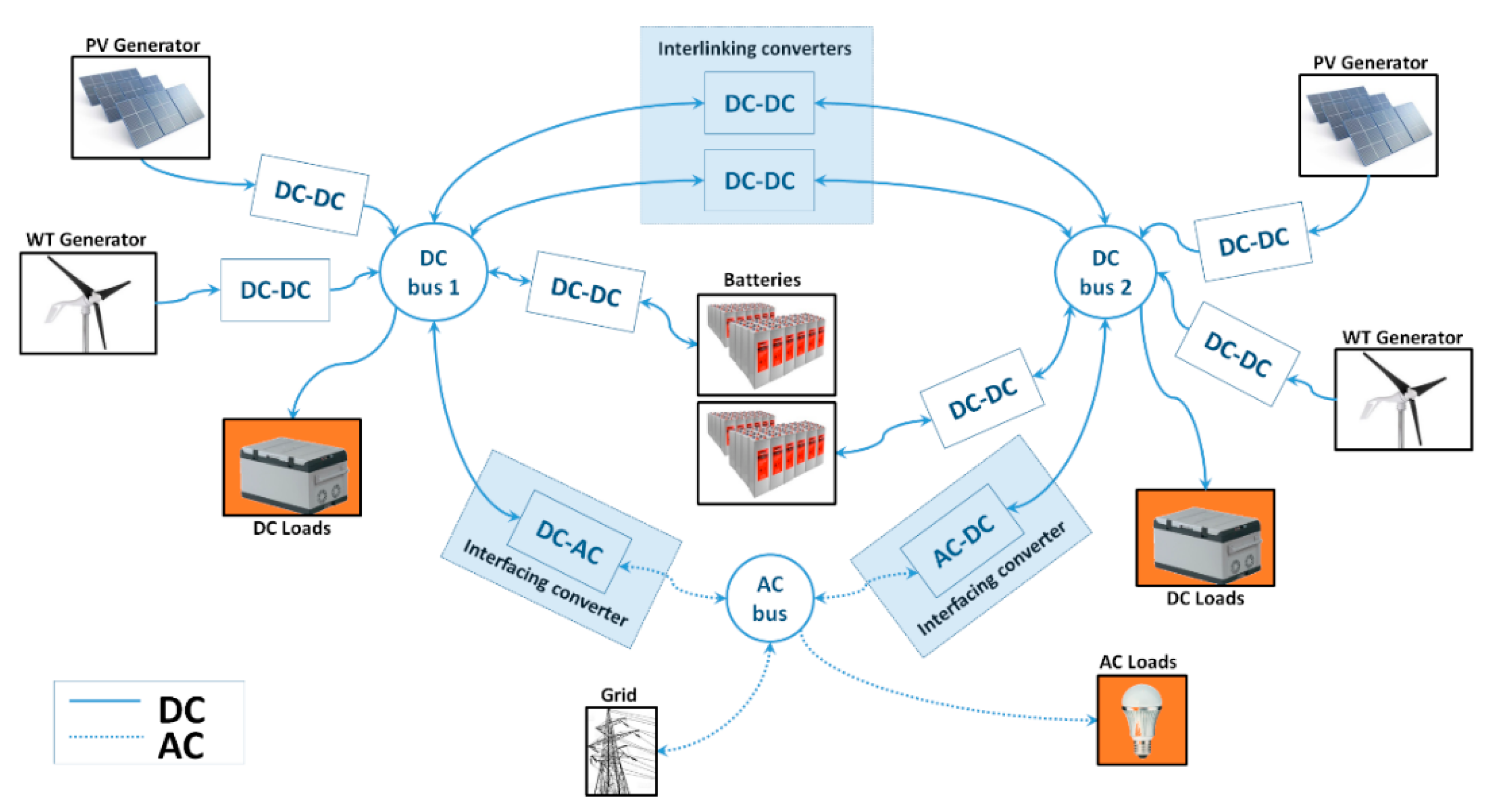
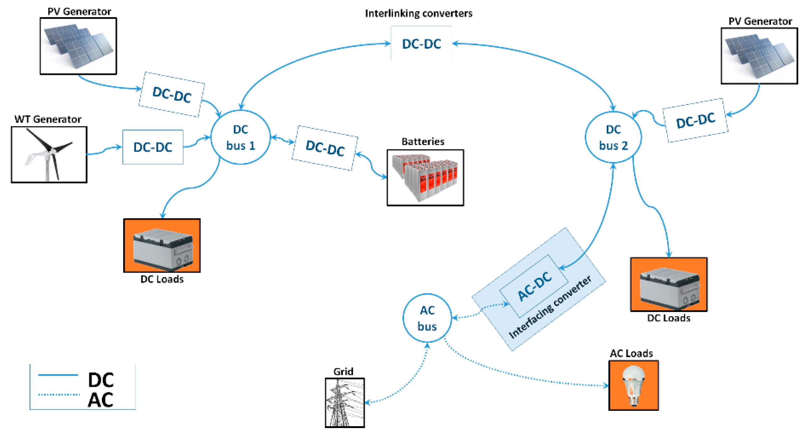
Diverging from the previously published approaches, this paper describes the development of a model for continuous simulation of a flexible architecture of hybrid microgrids integrating two DC buses and AC distribution. The main feature distinguishing the proposed simulation from those previously described is the simplicity of the used models, which are standardized to share power values as input and output variables. The programming of the block-based definition of the models allows the integration of multiple generators, energy storage units (ESU), and loads, configuring a control plant with a multiple-input multiple-output (MIMO) model able to apply different control approaches and validate its behavior. Additionally, because the model is focused on the real power flow, efficiency analysis of the microgrid can be easily derived.
The rest of the paper is organized as follows: Section 2 presents a description of the hybrid microgrid architecture selected as a case study. Section 3 details the modelling of the elements comprising the microgrid, and a detailed implementation description is presented in Section 4. Simulation results for different operation scenarios are provided, validating the correctness of the computation and the usefulness of the simulation application, in Section 5. Finally, conclusions and future work are summarized in Section 6.

2. Description of the Selected Microgrid Architecture

The model was developed considering a flexible architecture in which the majority of the concepts applied in microgrids can be studied. Because of this main feature, it also serves as a flexible basis for simulation of other simpler architectures of microgrids. The microgrid is composed of two DC distribution buses with different voltage levels and an AC bus. The AC bus is a standard single-phase point of common connection (PCC) interconnecting the microgrid, the grid, and AC loads. In Figure 1, the architecture of the hybrid microgrid selected as a case study is depicted.
Both DC buses of the microgrid are nodes integrating renewable generators, energy storage, and local loads. Photovoltaic modules (PV) and Wind Turbines (WT) are considered among the existing renewable energies. Each bus can integrate several generators, allowing the study of multiple control and energy management strategies. The microgrid uses energy storage units (ESU) connected to one of the DC buses; each DC bus can integrate multiple ESU. The loads connected to the buses are represented with a constant power behavior. The loads connected to the AC side can be fed by either the grid or the microgrid. They can be fed by the microgrid by using power converters taking the required energy from one or both DC buses. The exchange of energy between DC buses is enabled using one or two paralleled bidirectional DC–DC converters, named interlinking converters (ILC). The interaction between the DC buses and the AC bus is enabled by using bidirectional DC–AC converters, named as interfacing converters (IFC). Fundamentals considered in the architecture selection take the basis of the overview of power and control architectures presented in [10]. From a generalized perspective, the selected architecture allows the study of multiple alternatives for power flow into the microgrid, which are defined by the user through the rules programmed into the external decision algorithm as control. In this paper, we focus on the mathematical modelling of a hybrid microgrid as a plant with the aim to provide flexibility to the study’s multiple control strategies.

3. Modelling

The proposed model was built considering each component of the microgrid as a module with a mathematic model representing a power source or a power load. These modules were integrated through a generalized mathematic model of the microgrid buses and the control algorithms. For example, a battery module has a source behavior during the discharge process and a load behavior during the charging process, requiring that their model can consider bidirectional flow and different modes of operations. Similarly, although generators have a unidirectional power flow, they are composed of a chain of modules involving power production, efficiency profiles of the power converters, and the maximum power point tracking algorithms.
Mathematical expressions modelling different modules use numerical variables N p q x n z (taking values 0 and 1), allowing the configuration of different modes of operation. The sub-indexes p and q define the type of unit (PV: photovoltaic, WT: Wind, ES: Energy Storage), while x denotes the bus in which a unit is connected (1, 2 or 3), n defines the index if more than one unit of the same nature is connected to the same bus (1, 2, …), and z allows the differentiation of functions for each unit ( a , b , and c , if required). Using these signals, an external decision algorithm can control the power given or absorbed by each module. Similarly, the power variables are defined using the same convention with an added sub-index to identify the power in a conversion chain (1, 2 and 3).
The block diagrams used within the paper consider the results of computations at the right side of the blocks from the values available at the left side and the parameters selecting the operation modes. If computations consider the output value also as an input, the value corresponding to the previous sampling period is used as an input. The modelling for all modules used in the simulation is presented below.

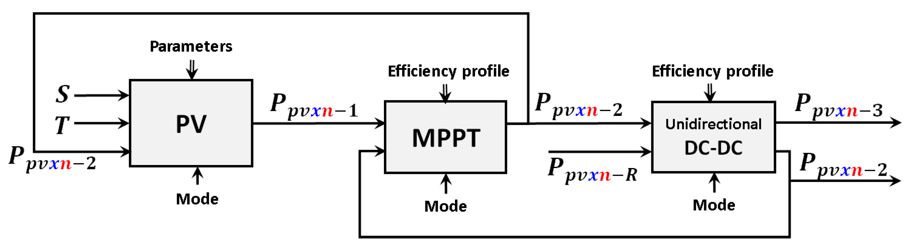
3.1. Modelling of the PVG

The power delivered by a PV generator depends on a chain composed by three modules: the solar panel, the maximum power point tracking (MPPT) algorithm, and one unidirectional DC–DC power converter. Integrated to a DC bus in the microgrid, each generator can operate in the three modes listed in Table 1. In the modes 0 and 3, the generator is deactivated and its power contribution is zero. Operating in the mode 1, the PV module delivers the maximum available power, which is affected by the MPPT efficiency and the DC–DC converter efficiency. Contrarily, operating in the mode 2, the solar panel delivers a fraction of the available power, tracking an external power reference given by a superior level of the control hierarchy of the microgrid. In mode 2, the power delivered by the solar panels is affected only by the efficiency of the DC–DC converter, as the MPPT algorithm does not operate (in this mode the MPPT efficiency is settled to 100%).

3.1.1. Solar Panel Model

A general but simple model of a photovoltaic panel calculating the maximum output power for specific irradiance and temperature values is given by the following expression:
P p v x n m a x = S p v S r e f P p v x n n o m 1 + γ T p v T r e f
where P p v x n m a x is the rated power of the PV module, S p v is the instantaneous irradiance, S r e f is the irradiance reference (1000 W/m2), T p v is the instantaneous temperature, T r e f is the temperature reference (25 °C), and γ is the maximum power correction factor for temperature, which takes values around −0.005, depending on the material employed to build the panel [39]. P p v x n n o m is the nominal power of the generator applied for both the PV module and power converter. Then, for a set of environmental conditions, this model provides the value of the maximum allowable power which can be extracted either totally or partially.

3.1.2. MPPT Algorithm

Conventionally, the efficiency of the MPPT algorithms used in PV applications depends on the irradiance level or consequently on the extracted power. This efficiency value can range from 80% to 99.9% in the more active MPPT algorithms [40,41]. Then, the efficiency of the MPPT is represented as a function of the maximum allowable power provided by the model of the PV module. As mentioned previously, the efficiency of the MPPT is settled to 100% when operating in the limited power mode. The MPPT efficiency profile of the PV generators can be loaded separately for each generator or unified for all generators integrated to a DC bus. The efficiency profile is defined by means of the coefficients A p v x n 1 and A p v x n 0 of the first order polynomial in (2), which depends on the relationship between the available power P p v x n 1 and the nominal power P p v x n n o m .
η p v x n m p p P p v x n 1   = A p v x n 1 P p v x n 1 P p v x n n o m + A p v x n 0

3.1.3. DC–DC Converter

To integrate PV generators into a DC bus of the microgrid, at least one DC–DC conversion stage is required. Regardless of the studied bus, the efficiency profiles of the converters are represented using static gains defined by first-order polynomials depending on the converted power. These profiles can be obtained from the results of laboratory tests measuring the efficiency of the converter for different output power values. The efficiency profile is defined by means of the coefficients B p v x n 1 and B p v x n 0 of the expression in (3), which depends on the relationship between the extracted power P p v x n 2 and the nominal power P p v x n n o m .
η p v x n d c P p v x n 2   = B p v x n 1 P p v x n 2 P p v x n n o m + B p v x n 0
At this point, it is also possible to compute the maximum power that can be provided by a PV generator in the mode 2 which corresponds to the maximum power at a defined operation point directly affected by the efficiency of the converter η p v 12 d c 1 . It is important to mention that the generator may be unable to provide the power defined by the external reference, in which case it will provide a power near to the maximum allowable.
η p v x n d c 1 P p v x n m a x   = D p v x n 1 P p v x n m a x P p v x n n o m + D p v x n 0
P p v x n a u x = max P p v x n m a x η p v x n d c 1 P p v x n m a x ,   P p v x n r e f
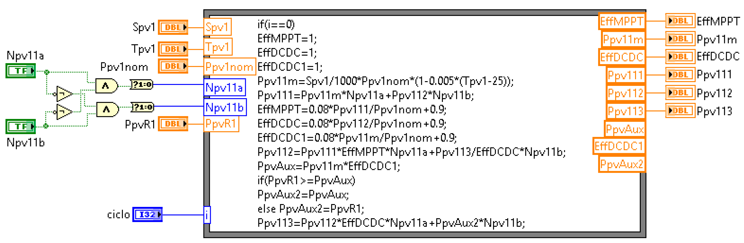
The complete modelling of the PV generators is synthesized in Expressions (6)–(8) computing the output of each block. P p v x n r e f is a power reference given by an outer loop regulating the bus voltage or by a superior layer in the hierarchical architecture of the microgrid control.
P p v x n 1 k   = P p v x n m a x N p v x n a + P p v x n 2 k 1 N p v x n b
P p v x n 2 k   = P p v x n 1 η p v x n m p p N p v x n a + P p v x n 3 k 1 / η p v x n d c N p v x n b
P p v x n 3 k   = P p v x n 2 η p v x n d c N p v x n a + P p v x n a u x k 1 N p v x n b
The resulting assembly of blocks conforming PV generators is depicted in Figure 2, showing the causal flow of the required computations.

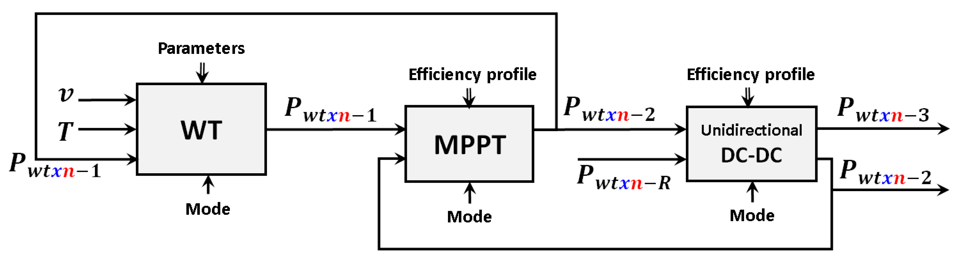
3.2. Modelling of the WTG

The power delivered by a wind generator depends on the chain composed of the following three modules: the wind turbine, the MPPT algorithm, and the power converter which is composed of an AC–DC stage and a DC–DC stage. The wind generator can operate in the modes listed in Table 2. In the modes 0 and 3, the generator is deactivated and its power contribution is zero. In the MPPT mode (namely mode 1), the generator delivers the maximum available power, which is affected by the MPPT efficiency and the AC–DC–DC converter efficiency. Operating in the mode 2, the wind generator delivers a fraction of the available power, tracking an external power reference. In this mode, the power delivered is affected only by the efficiency of the AC–DC–DC converter.

3.2.1. Wind Turbine

The wind turbine static behavior can be modelled by the piece-wise function in Expression (9) defining the produced power as a function of the wind speed besides some parameters from the geometry and size of the turbine. The conventional model defining this curve requires the cut-in speed v c i n , the nominal speed v r a t , and the cut-out speed v c o u t of the turbine as follows:
P W T = 0 0 < v v c i n 0.5 ρ A C p v 3 v c i n < v v r a t P r a t v r a t < v v c o u t
where v is the wind speed, ρ the air density, A the area swept by the rotor blades, C p the power coefficient of the turbine, and P r a t the nominal power [42]. A simplified version of this model is obtained following the shape of the saturation function as follows:
P w t x n = 0 0 < v < V m i n P m a x V m a x V m i n v P m a x V m i n V m a x V m i n V m i n v V m a x P m a x V V m a x
where the resulting piecewise model is defined by the coordinates V m i n , 0 and V m a x , P m a x .

3.2.2. MPPT Algorithm

The efficiency of the MPPT algorithms for wind generators depends on the wind speed or consequently depends on the extracted power. In a practical sense, the same algorithms used for PV generators can be used for wind turbines. The first order expression in (11) models the efficiency of that algorithm as a function of the rated power.
η w t x n m p p P w t x n 1 = A w t x n 1 P w t x n 1 P w t x n n o m + A w t x n 0

3.2.3. AC–DC–DC Converter

Low-power wind generators are commonly built integrating a Permanent Magnet Synchronous Generator (PMSG) to provide the conversion of mechanical energy into electrical energy. These generators have a three-phase AC output whose voltage and power depend on the wind speed and the connected load. Therefore, to integrate a wind generator into a DC bus of the microgrid, an AC–DC converter is required. The simpler topology is a two-stage power conversion chain composed by a three-phase diode bridge rectifier and a boost-type DC–DC converter, the second allowing the control of the extracted power. The efficiency profile is defined by means of the coefficients B w t x n 1 and B w t x n 0 of the first order polynomial in (12), which depends on the relationship between the extracted power P p v x n 2 and the nominal power P w t x n n o m .
η w t x n d c P w t x n 2   = B w t x n 1 P w t x n 2 P w t x n n o m + B w t x n 0
At this point, it is possible also to compute the maximum power that can be provided by the WT generator in the mode 2, which corresponds to the maximum power at a defined operation point directly affected by the efficiency of the converter η w t x n d c 1 . It is important to mention that the generator may be unable to provide the power defined by the external reference, in which case it will provide a power near to the maximum allowable.
η w t x n 1 P w t x n m a x   = B w t x n 1 P w t x n m a x P w t x n n o m + B w t x n 0
P w t x n a u x = max P w t x n m a x η p v x n 1 P w t x n m a x ,   P w t x n r e f
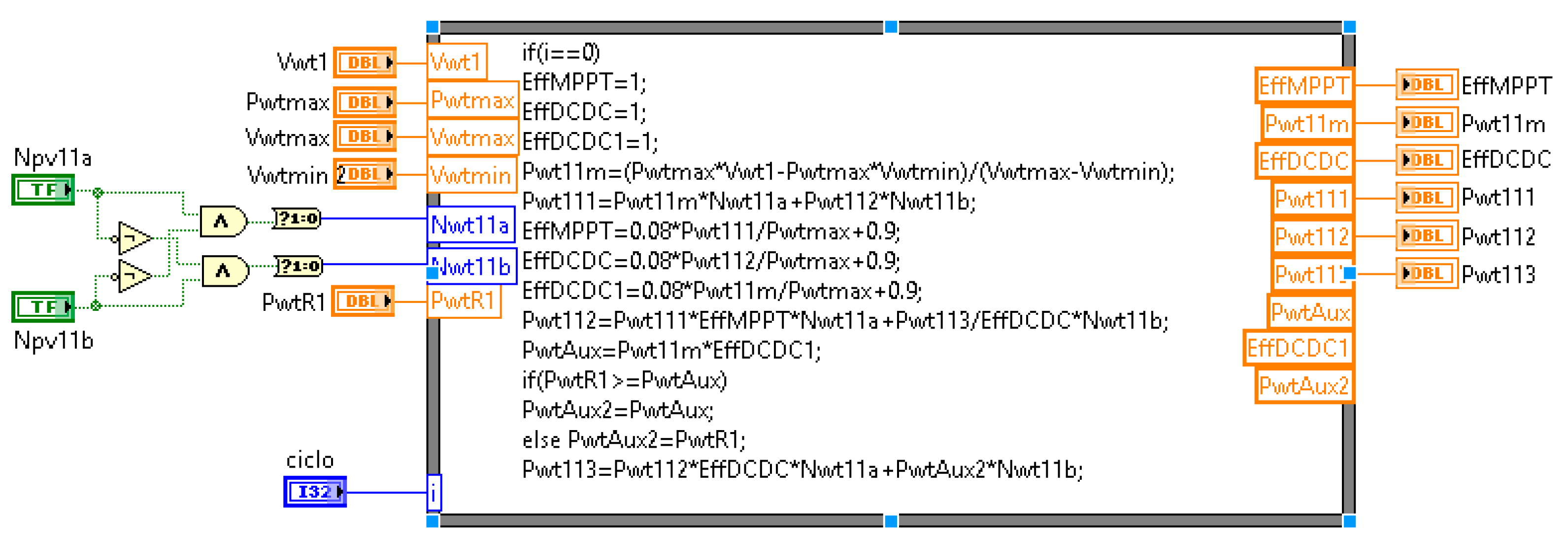
The complete modelling of the WT generators can be synthesized in Expressions (15)–(17), computing the output of each block. P w t x n R is a power reference given by an outer control loop.
P w t x n 1 k   = P w t x n v , T N w t x n a + P w t x n 2 k 1 N w t x n b
P w t x n 2 k   = P w t x n 1 η m p p t + P w t x n 2 k 1 / η w t x n d c N w t x n b
P w t x n 3 k   = P w t x n 2 η w t x n d c N w t x n a + P w t x n a u x k 1 N w t x n b
By assembling the three described modules, the wind generators (WTG) are modelled as depicted in the block diagram presented in Figure 3. Equivalent to the PV generators, the x sub-index defines the bus in which the generator is connected, and the n sub-index differentiates the generators connected to the same bus.

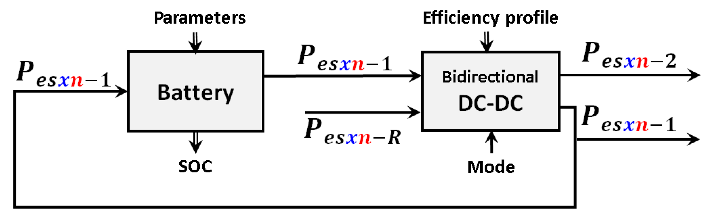
3.3. Modelling of the ESU

An Energy Storage Unit (ESU) is composed of a battery array and a bidirectional DC–DC converter which controls its charge/discharge regimes. An ESU can operate in the modes listed in Table 3. In the modes 0 and 3, ESU is deactivated. In the mode 1, batteries are charging according to the external power reference given by control. The maximum power injected is normally defined as a percentage of the nominal capacity given in Amperes multiplied by the charging voltage. This mode can remain active until the battery is charged to a desired level. In the mode 2, batteries are discharged, injecting power into the bus in which the ESU is connected. In this mode, the amount of power delivered by the ESU is defined by an outer reference which can be used to establish the power balance on the bus.

3.3.1. Batteries

To model the ESU, the State of Energy (SoE) indicator is selected [43]. As it can be shown in (18), the battery power is affected by the efficiency factor η e into the integral term, which allows the establishment of the similitude with the previously defined models of the simulation. The SoE can be defined as:
S o E = 1 + 0 t 1 η e P t E n ·   100 %

3.3.2. Bidirectional DC–DC Converter

The bidirectional DC–DC converter used in the ESU can transfer power from the bus to the battery and from the battery to the bus. Normally, the charging process requires a predefined amount of power established by the charge regime (constant current or constant power), but it can also be made using a different amount of power if the ESU regulates the voltage of the bus. The efficiency profile of the converter is separately defined for each power flow direction, as normally the voltage level of the buses differs from the voltage level of the battery array. Then, simulation differentiates the efficiency profiles η d c d c 2 P b t x n 1 and η d c d c 1 P b t x n 2 
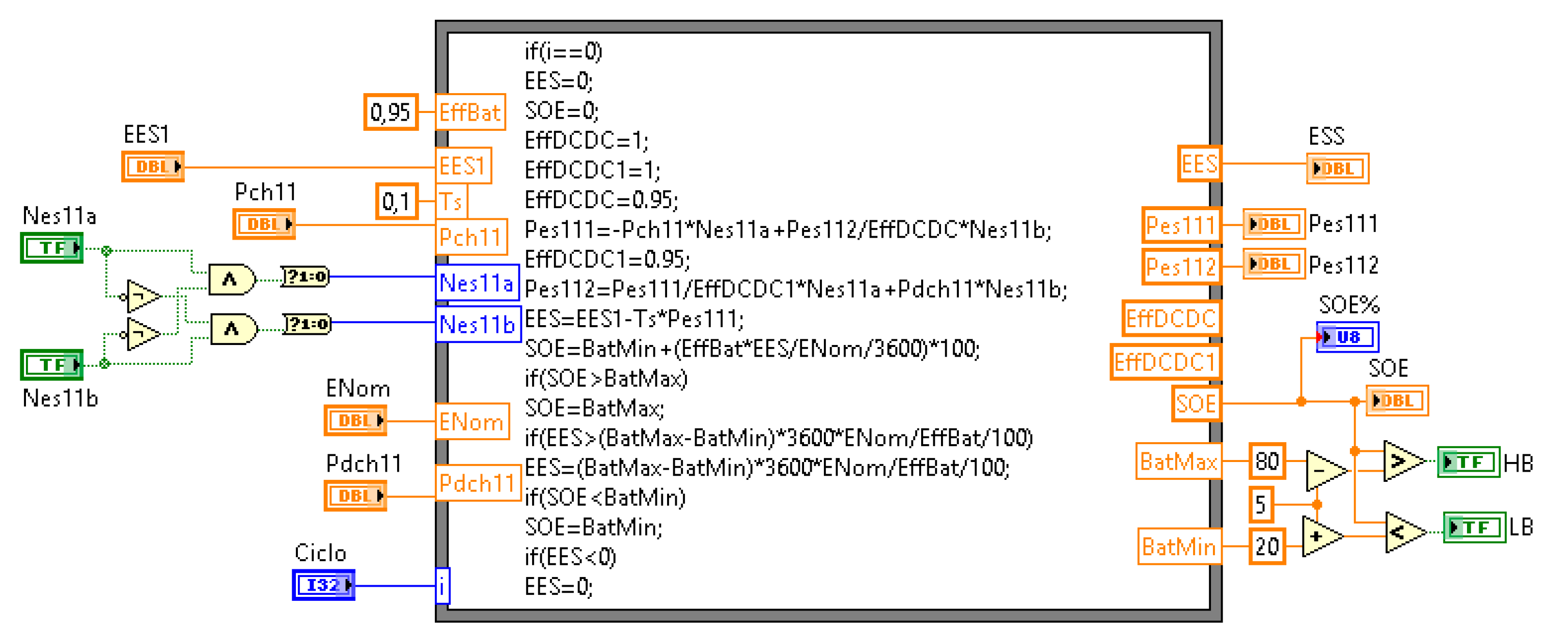
for charging and discharging modes, respectively, using expressions with the form of (3). The complete modelling of the ESU can be synthesized in Expressions (19) and (20) computing the output of each block. P b t x n R is a power reference given by an outer loop regulating charge and discharge processes.
P e s x n 1 k   = P e s x n I c h m a x , V b a t N e s x n a P e s x n 2 / η d c d c 1 N e s x n b
P e s x n 2 k   = P e s x n 1 / η d c d c 2 N b t x n a + P e s x n R k 1 N b t x n b
By assembling the two described modules, an ESU is modelled as it is depicted in the block diagram presented in Figure 4.

3.4. Modelling of the Power Consumption

The DC loads can be classified into three types: constant resistive load (CRL [44]), constant current load (CCL [45]), and constant power load (CPL [46]). The AC loads are classified into resistive, inductive, capacitive, or nonlinear groups [47]. The simulation considers the real power consumption of the loads in both DC and AC buses as a constant value that can suffer changes representing connection or disconnection of loads. The convention used by the model is P L x .

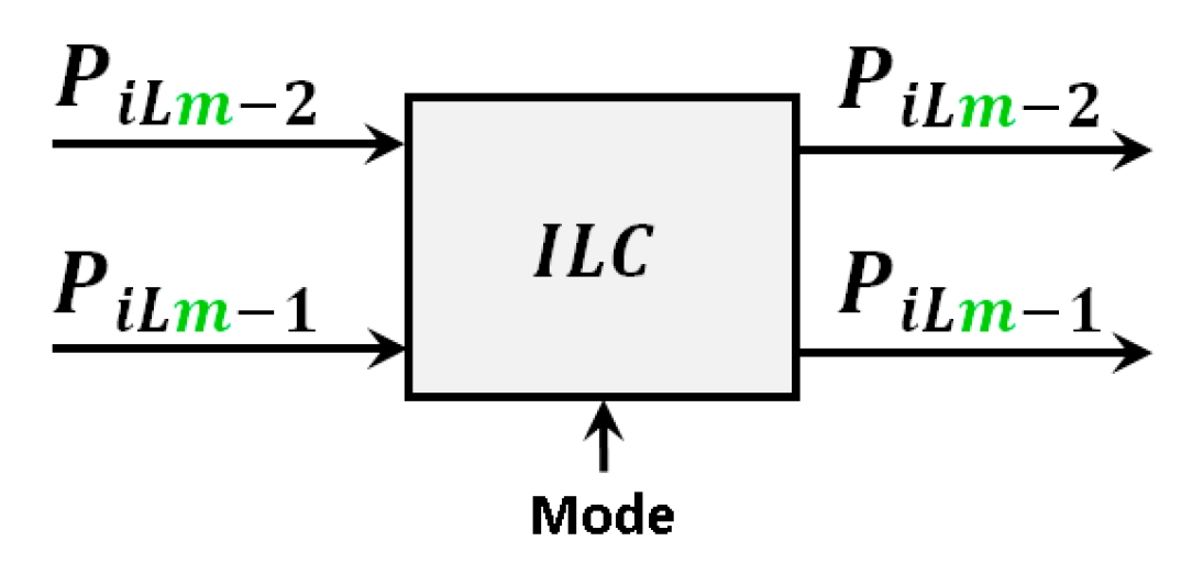
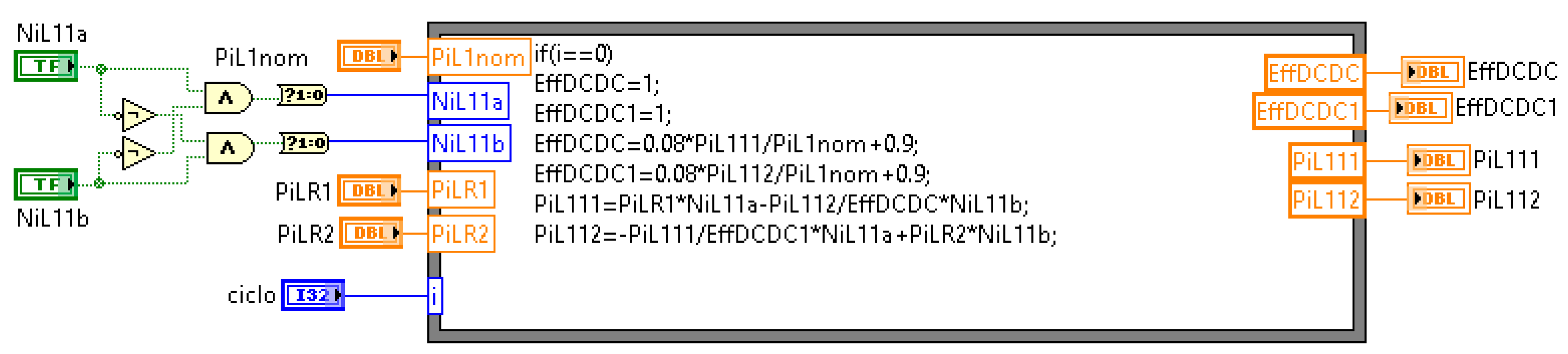
3.5. Modelling of the ILCs

The DC buses 1 and 2 can exchange power through the ILCs. Therefore, these converters are able to operate with bidirectional power flow. Considering voltage levels of the DC buses are regulated, the efficiency profile of these converters are defined by two curves with the form defined by (3). The possible modes of operation of this converter are listed in Table 4. When the IFC is operating in mode 0, the DC buses of the microgrid are disconnected, which in fact decouples their operation. In the modes 1 and 2, the converter transfers power from one DC bus to the other.
The simulation differentiates the efficiency profiles η d c d c 1 P i L m 1 and η d c d c 2 P i L m 2 for different modes, respectively. The following set of expressions allows the computation of the power at both ports of one ILC.
P i L m 1 k   = P i L m R 1 N i L m a + P i L m 2 k / η d c d c 2 N i L m b
P i L m 2 k   = P i L m 1 k / η d c d c 1 N i L m a + P i L m R 2 N i L m b  
where P i L m R 1 and P i L R 2 are the power references given by an outer control loop to define the amount of power transferred by one ILC. Parameters N i L m a and N i L m b define the priority of the ILCs, indicating which of the two ports fixes the required or demanded power and allowing the computation of the power in the other port. A block diagram of the model of the ILCs is depicted in Figure 5.

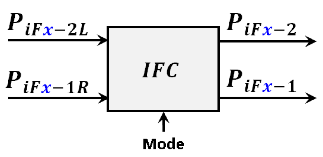
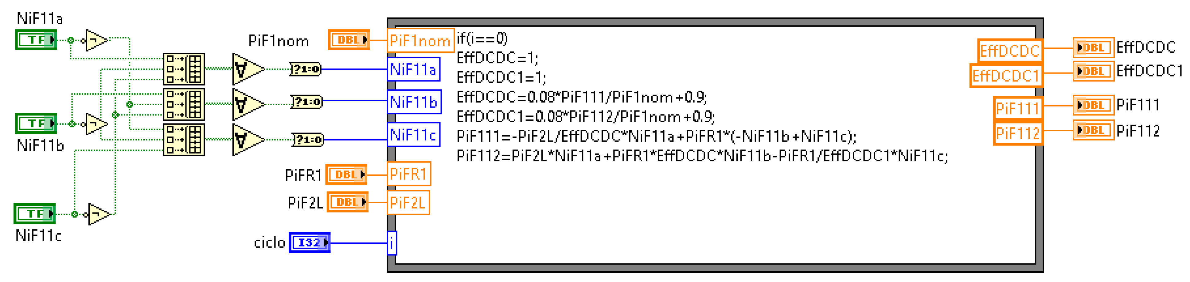
3.6. Modelling of the IFCs

The DC buses are connected to the AC side of the microgrid through the IFCs. These converters are able to operate with bidirectional power flow. However, when they operate connected to the auxiliary generator, the flow is limited to transfer power from the generator to the microgrid. As shown in Table 5, these converters have four operation modes. When the converter is OFF, the AC loads can only be fed directly from the grid or the generator. When the IFCs are operating in stand-alone mode (mode 1), they feed the AC loads. In modes 2 and 3, the IFCs are connected to the auxiliary generator or to the grid, and they establish the power balance of the DC buses.
A conditional logic was designed to avoid other possible modes resulting from undesired combinations of the N i f c x a values. The efficiency profiles of the IFCs are defined separately for operation in the two possible power directions. The efficiency profiles η d c a c x P i F x 1 and η a c d c x P i F x 2 have the form defined by Expression (3). The following set of expressions allows for the computation of the power at both ports of the IFCs.
P i F x 1 k   = P i F x 2 L / η a c d c N i F x a + P i F x R 1 k N i F x b + N i F x c
P i F x 2 k   = P i F x 2 L k N i F x a + P i F x R 1 k / η a c d c N i F x b P i F x R 1 k η d c a c N i F x c
where P i f c x 1 R is the power reference given by the control to define the amount of power transferred by the IFCs to or from a DC port and P i F x 2 L is the power load fed at the AC side (see Expressions (25) and (26)). Parameter N i F x a indicates if one IFC is operating in SAC mode while parameters N i F x b and N i F x c define the priority of the ILCs, indicating which of the two ports fixes the demanded or delivered power. A block diagram of the model of the IFCs is depicted in Figure 6.

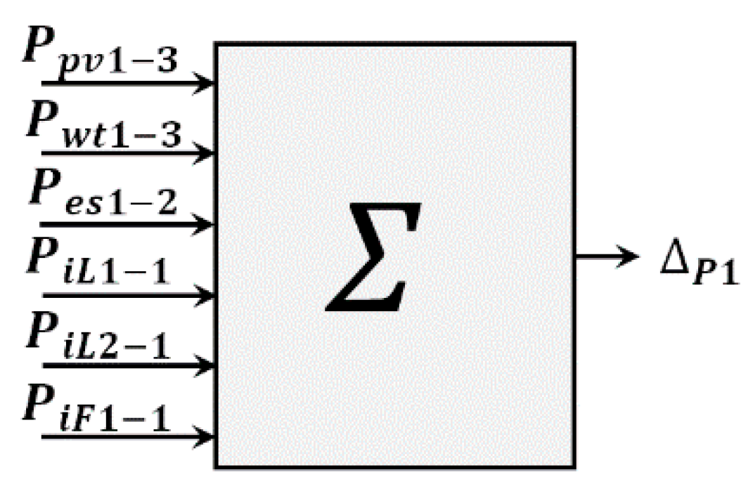
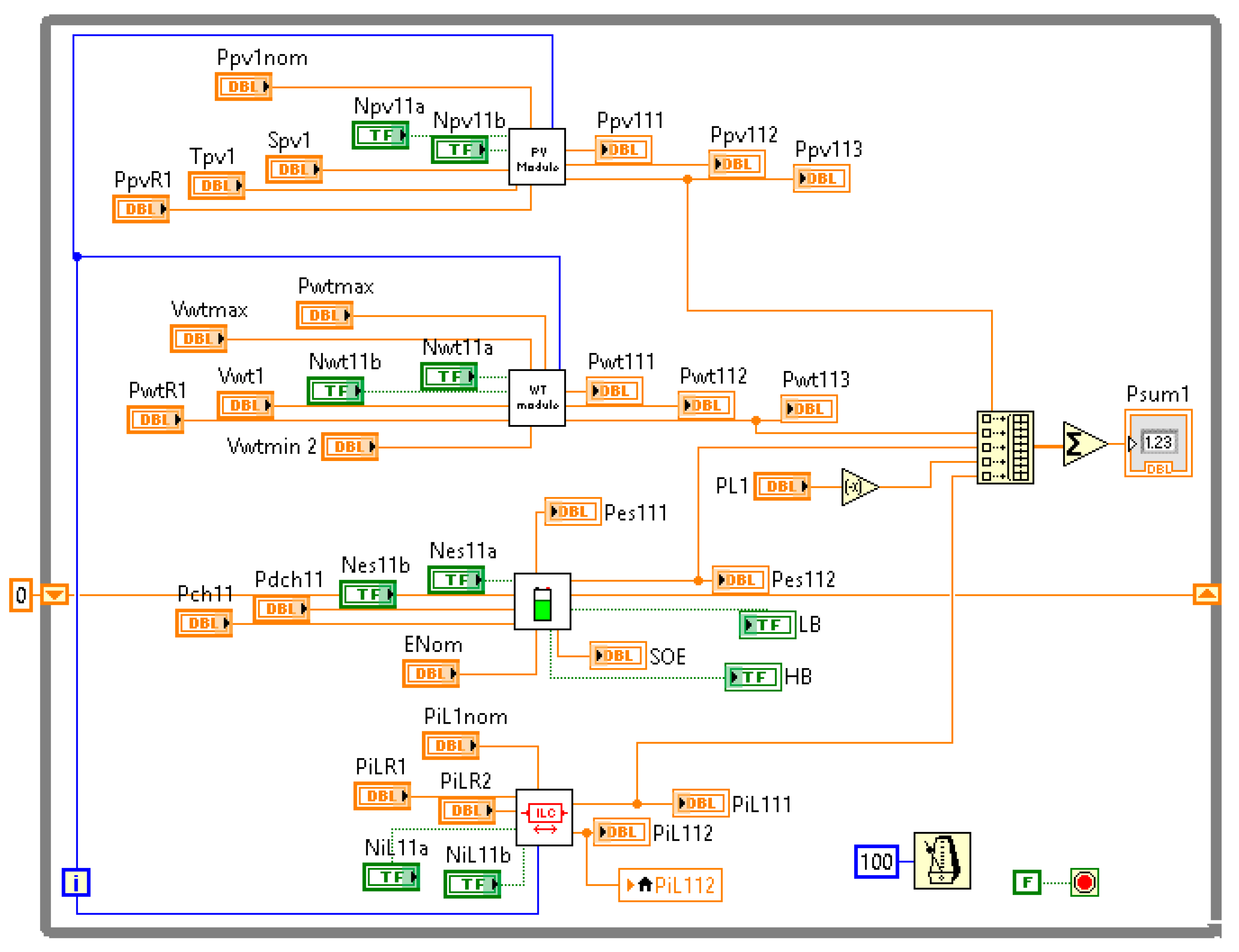
3.7. Modelling of the DC Buses

The DC buses allow the interconnection of the generation, storage, and consumption units. Each DC bus also integrates the power injected or extracted by one IFC and two ILCs. The model of each bus computes the instantaneous power balance defined by the variable Δ P 1 providing information to define the references of the control. A block diagram of the model corresponding to the DC bus 1 is depicted in Figure 7.

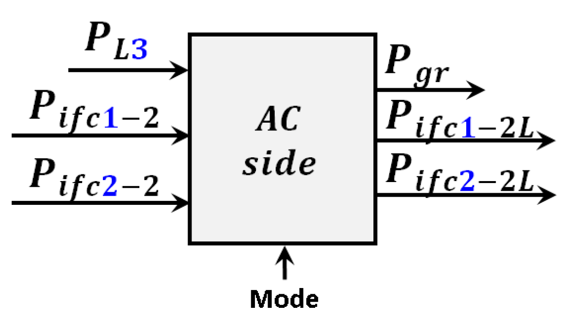
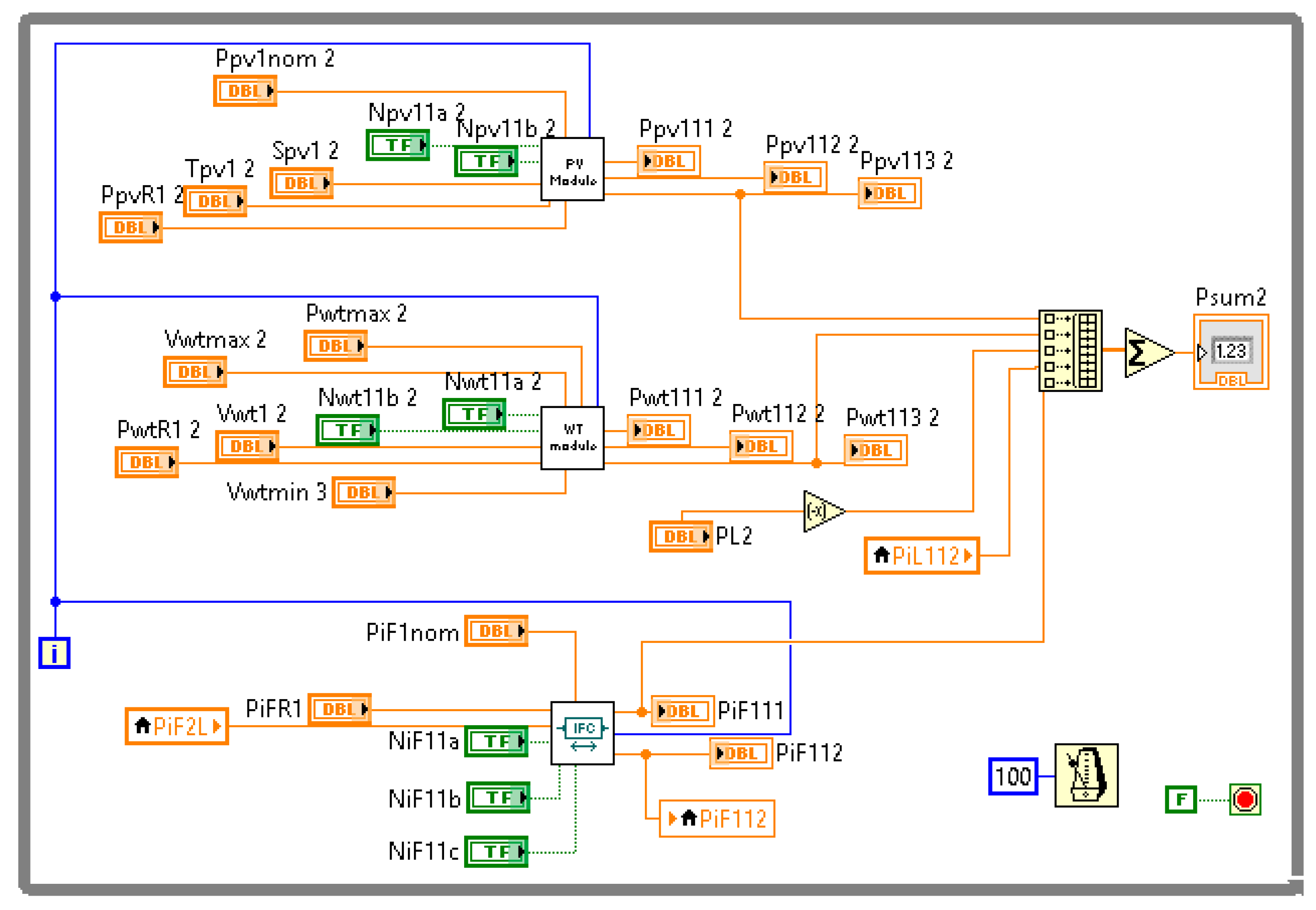
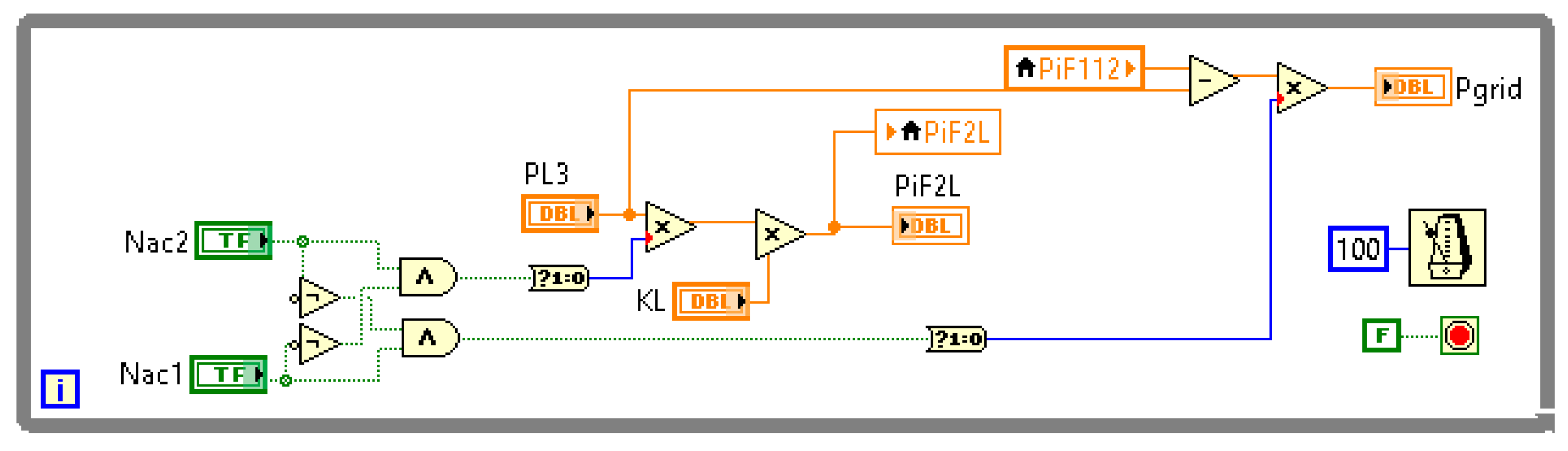
3.8. Modelling of the AC Side Interconnection

In the studied microgrid architecture, it is possible to feed the AC power consumption from three sources: the AC grid, an auxiliary fuel generator, and the DC buses through the IFCs operating in SAC mode. The presence of the AC grid and the auxiliary generator will determine if the AC load consumption P L 3 will be covered directly from them or indirectly through one or both of the IFCs. The following expressions allow modelling of the AC side of the microgrid:
P i F 1 2 L k   = P L 3 N a c 2 K L
P i F 2 2 L k   = P L 3 N a c 2 1 K L
The parameter K L is defined as the sharing index taking values between zero and one and defines the percentage of contribution of the IFCs operating as SAC feeding the loads. N a c 3 is an integer variable taking values into the set 0 ,   1 and defining the operation of the IFC in SAC mode. The power of the AC sources is defined by:
P g r k   = P L 3 N a c 2 + ( P i f c 1 2 k + P i f c 2 2 k ) N a c 1
Parameter N a c x defines which AC source fed the loads. Table 6 summarizes the connection/disconnection logic of the AC side.
A block diagram of the model of the AC side is depicted in Figure 8.

3.9. Modes of Operation and Special Features of the Simulated Microgrid

By considering the multiple modes of operation of the different units of the microgrid, the whole operation can be configured, but is not limited to operate in the following modes:
  • Islanded/DC (ISL-DCO): There is no AC source and the microgrid cannot produce enough energy to feed the AC loads, feeding the DC loads as priority.
  • Islanded/SAC (ISL-SAC): There is no AC source but the local generation is enough to feed both the DC and AC loads.
  • Grid/Grid (GRD/GRD): In this case, the grid has good quality and shares power consumption with the microgrid, which transfers power through the IFC.
A list of the suggested modes of operation is presented in Table 7 (Table 1, Table 2, Table 3, Table 4, Table 5 and Table 6 define the conventions of the modes and the corresponding values of N x x x for each of them).

4. Simulation Implementation

The simplified model developed in this work was implemented in a virtual instrument in the LabVIEW platform to obtain the continuous property. The main specifications for the software development were:
  • The user configures the parameters of the models of solar panels, wind turbines and batteries.
  • The user provides the coefficients of efficiency profiles of power converters and MPPT algorithms.
  • The user can change online environmental variables and power consumptions.
  • The simulation can interact with other algorithms through global variables.
The microgrid architecture depicted in Figure 9 was selected to provide details of the model programming. As it can be observed, the example has one PVG and one WTG integrated in the DC bus 1, one ESU integrated in the DC bus 1, one PVG integrated in the DC bus 2, one ILC interconnecting the DC bus 1 and the DC bus 2, and one IFC interconnecting the DC bus 2 with the AC bus. The programed functions developed for each of these units are shown in Figure 10, Figure 11, Figure 12, Figure 13 and Figure 14. Please consider that unlike the other units, programming of the ESU requires the creation of a shift register to obtain the delayed sample required to implement the integral function of the SoE ( E S S = S o E k and E E S 1 = S o E k 1 ).
As the different modules were programmed as subVis (in the context of LabVIEW programming), they could be inserted into the model of the whole microgrid, which was developed using three whole loops running separately (one loop per bus as shown in Figure 15, Figure 16 and Figure 17). The variables shared between buses through the ILC and IFC units were programmed as local variables. The loads connected to the buses were implemented as input variables. Controls and indicators used in the simulation were placed into a user interface, which is depicted in Figure 18.

5. Numerical Examples

5.1. Parameters of the Simulation

Simulations considered 250 W commercial solar panels [48], 300 W Permanent Magnet Generator Wind Turbines [49], and 12 V batteries with capacities of 100 Ah [50]. The main parameters are summarized in Table 8.
To facilitate correctness of the computations in the simulation, the efficiency of the MPPT and the efficiency profiles of all converters were defined by the following expressions using only the first order and constant terms:
η m p p t P x   = η c o n v e r t e r P x   = 0.08 P x P n o m + 0.9
where P n o m is the nominal power of the converter, which is defined as 3 kW.

5.2. Test Using Predefined Scenarios

Three scenarios were chosen for tests providing simulated results: Grid-connected GRD-GRD (night), Grid-connected GRD-GRD (day), and Islanded mode (ISL-SAC). The possible configurations of the microgrid to face each scenario are uncountable. A definition of the modes in which the units must operate to face each one of the selected scenarios is given in Table 9 (take this configuration only as example).
  • GRD-GRD (night): In this scenario, the complete operation of the microgrid is required because of the connection of loads to the three buses. The IFCs operate in grid-connected mode either as inverters or rectifiers. The ESU is settled to charging mode.
  • GRD-GRD (day): Similar to the previous scenario, the complete operation of the microgrid is required to feed the connected loads. The IFCs operate in grid-connected mode either as inverters or rectifiers. The ESU is settled to charging mode.
  • ISL-SAC: In this scenario, the microgrid operates without AC power supplied from the grid but the AC loads are fed by the IFC, which operates as SAC. The IFC cannot regulate the voltage of the DC bus 2, forcing the ILC to perform this task. As a consequence, the voltage of the DC bus 1 is regulated by the ESU, which can pass from a charging mode to a discharging mode depending on the renewable energy production which operates at MPPT.

5.2.1. Results for Scenario 1: Operation in GRD-GRD (Night)

In this scenario, the PVGs were off and the WTG contributed to the DC bus 1 with powers between 1500 and 2500 W. The total consumption of the loads into the microgrid varied between 2000 and 5000 W. The resulting power values establishing the stable operation of the microgrid in the example are presented in Table 10.
In this scenario, voltage regulation of the DC bus 1 was performed by the ILC while the voltage regulation of the DC bus 2 was performed by the IFC. In the three cases, the deficit of power was covered from the grid. In the first case, the efficiency was computed as 91.7%. In the second case, the efficiency was computed as 87.5%. In the third case, the efficiency was computed as 80%. As expected, these are the results obtained using the control rules manually provided to the simulation, which do not use the ESU to cover consumption. Then, for the other set of control rules, for example, the consumption of the DC bus 1 can be covered from the ESU while the consumption of the DC bus 2 is covered from the grid.

5.2.2. Results for Scenario 2: Operation in GRD-GRD (Day)

In this scenario, the microgrid fed the same power loads as in the cases of the previous scenario. The PVGs contributed with powers between 500 and 1500 W and the WTG contributed to the DC bus 1 with three different powers between 1300 and 2500 W. The total consumption of the loads into the microgrid varied between 2000 and 5500 W. The resulting power values establishing the stable operation of the microgrid in the example are presented in Table 11.
In this scenario, regulation of the buses was performed in the same way as it was performed for the scenario 1. In the three cases, the deficit of power was covered from the grid. In the first case, the efficiency was computed as 85.2%. In the second case, the efficiency was computed as 88%. In the third case, the efficiency was computed as 83.8%. As expected, these are the results obtained using the control rules manually provided to the simulation, which do not use the ESU to cover consumption. Then, for the other set of control rules, for example, the consumption of the DC bus 1 can be covered from the ESU while the consumption of the DC bus 2 is covered from the grid.

5.2.3. Results for Scenario 3: Operation in ISL-SAC Mode

In this scenario, the microgrid fed the same power load as in the previous scenarios. The PVGs contributed with powers between 1000 and 1500 W while the WTG contributed with powers between 1000 and 2500 W. The resulting power values establishing the stable operation of the microgrid in the control example are presented in Table 12.
In this scenario, voltage regulation of the DC bus 1 was performed by the ESU1 while the voltage regulation of the DC bus 2 was performed by the ILC1. The IFC1 was deactivated while the IFC2 operated as SAC, feeding the AC load. In the three cases, the power consumption was entirely covered by the microgrid. The efficiency was computed as 86%, 80.5%, and 84.4% for each case, respectively.

6. Conclusions

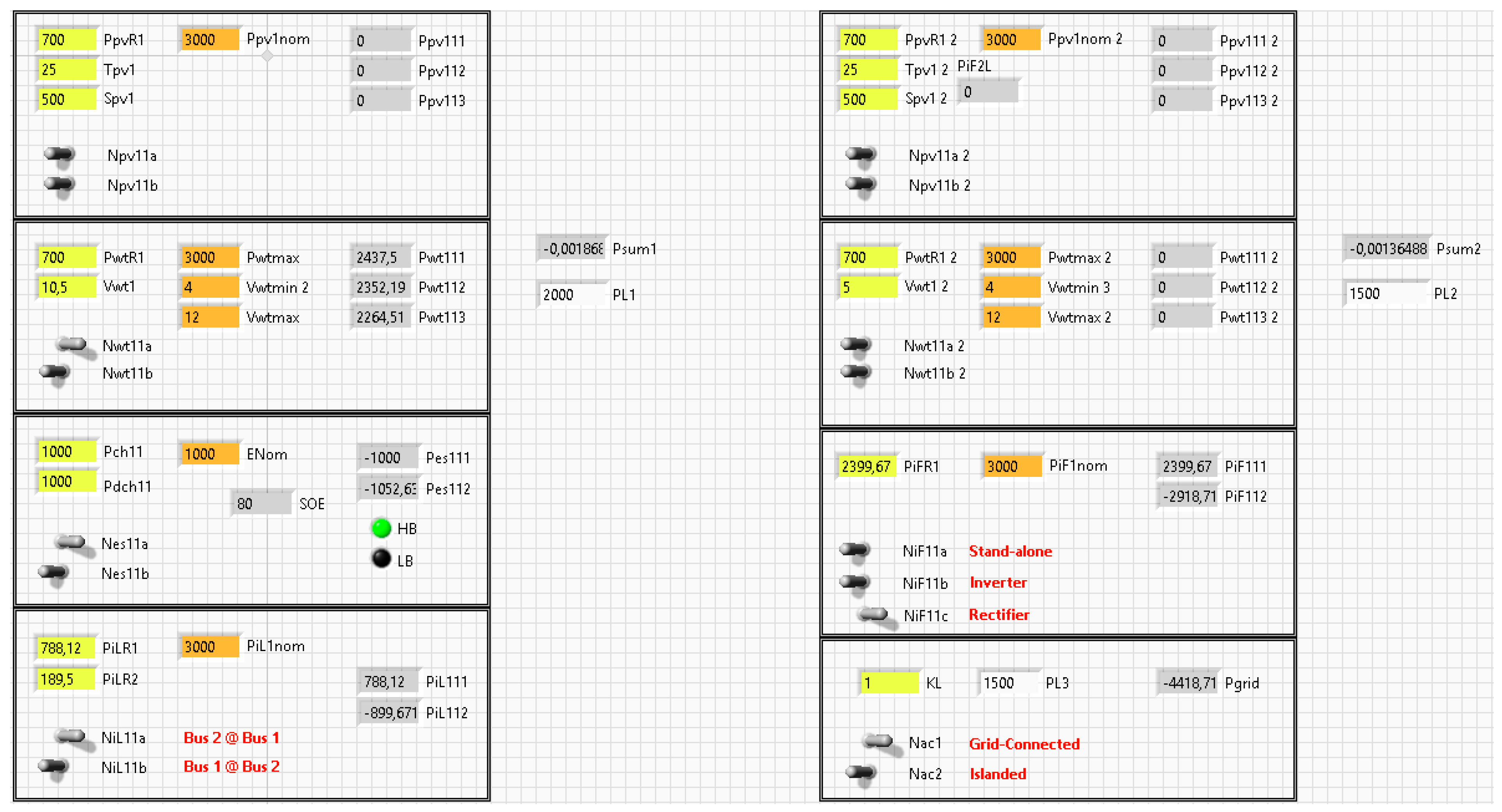
A flexible and simple model was proposed in this paper, allowing for the easy simulation of the power flow behavior for hybrid microgrids. The use of simplified models of solar panels, wind turbines, batteries, and loads and a binary logic to configure the operation of the microgrid allowed us to considerably reduce the computational cost of the simulation. Complementarily, the use of efficiency profiles to accurately model power-processing stages and MPPT algorithms increased the accuracy of the simulation without increasing its complexity, and allowed us to evaluate the efficiency of the entire microgrid for the studied scenarios and cases, providing elements to analyze how to improve the whole performance of the system. Simulated models were implemented in LabVIEW software.
Simple control rules ensuring power balances in DC and AC buses were used to test the functionality of the model in examples for three different scenarios (night and day operation having grid connection and islanding mode feeding AC loads) and three different cases in each of them, in which differences were introduced for power production and consumption. The power flow of the microgrid was analyzed from the power transferred by the IFC and ILC bidirectional converters.
As a relevant contribution to the study of microgrids, this simulation can operate as a model with input parameters and variables and output variables able to interact with other algorithms performing control functions. Moreover, the results showed the potentiality of the proposed model to serve as a plant to study the application of control algorithms in both educational and research environments.

Author Contributions

All authors contributed equally to all the stages of the research process and the preparation of the manuscript. All authors have read and agreed to the published version of the manuscript.

Funding

This research was developed with the partial support of the Ministerio de Ciencia, Tecnología e Innovación de Colombia (MinCiencias) under contract 018–2016.

Institutional Review Board Statement

Not applicable.

Informed Consent Statement

Not applicable.

Data Availability Statement

Not applicable.

Conflicts of Interest

The authors declare no conflict of interest.

References

  1. Chang, L. Editorial Special Issue on Resilient Microgrids. IEEE J. Emerg. Sel. Top. Power Electron. 2016, 4, 1145–1146. [Google Scholar] [CrossRef]
  2. Madduri, P.A.; Poon, J.; Rosa, J.; Podolsky, M.; Brewer, E.A.; Sanders, S.R. Scalable DC Microgrids for Rural Electrification in Emerging Regions. IEEE J. Emerg. Sel. Top. Power Electron. 2016, 4, 1195–1205. [Google Scholar] [CrossRef]
  3. Shahidehpour, M.; Pullins, S. Microgrids, Modernization, and Rural Electrification. IEEE Electrif. Mag. 2015, 3, 2–6. [Google Scholar] [CrossRef]
  4. Gaona, E.; Trujillo, C.; Guacaneme, J. Rural microgrids and its potential application in Colombia. Renew. Sustain. Energy Rev. 2015, 51, 125–137. [Google Scholar] [CrossRef]
  5. Battaiotto, P.E.; Cendoya, M.G.; Toccaceli, G.M.; Vignoni, R.J. Stand-alone hybrid microgrid for remote areas. Topology and operation strategy. In Proceedings of the IEEE URUCON, Montevideo, Uruguay, 23–25 October 2017; pp. 1–4. [Google Scholar]
  6. Prakash, S.S.; Mamun, K.A.; Islam, F.R.; Cirrincione, M. Design of a Hybrid Microgrid for a Rural Community in Pacific Island Countries. In Proceedings of the 4th Asia-Pacific World Congress on Computer Science and Engineering (APWC on CSE), Mana Island, Fiji, 11–13 December 2017; pp. 246–251. [Google Scholar]
  7. Roy, H.S.; Sarker, M.R.; Ahmed, T. Design and Analysis of Future Hybrid Micro Grid System for Matiranga. In Proceedings of the IEEE Region 10 Symposium (TENSYMP), Dhaka, Bangladesh, 5–7 June 2020; pp. 896–899. [Google Scholar]
  8. Hossain, E.; Kabalci, E.; Bayindir, R.; Perez, R. Microgrid testbeds around the world: State of art. Energy Convers. Manag. 2014, 86, 132–153. [Google Scholar] [CrossRef]
  9. Lidula, N.W.A.; Rajapakse, A. Microgrids research: A review of experimental microgrids and test systems. Renew. Sustain. Energy Rev. 2011, 15, 186–202. [Google Scholar] [CrossRef]
  10. Nejabatkhah, F.; Li, Y.W. Overview of Power Management Strategies of Hybrid AC/DC Microgrid. IEEE Trans. Power Electron. 2015, 30, 7072–7089. [Google Scholar] [CrossRef]
  11. Loh, P.C.; Li, D.; Chai, Y.K.; Blaabjerg, F. Autonomous Operation of Hybrid Microgrid with AC and DC Subgrids. IEEE Trans. Power Electron. 2013, 28, 2214–2223. [Google Scholar] [CrossRef]
  12. Aljohani, T.M.; Ebrahim, A.F.; Mohammed, O. Hybrid Microgrid Energy Management and Control Based on Metaheuristic-Driven Vector-Decoupled Algorithm Considering Intermittent Renewable Sources and Electric Vehicles Charging Lot. Energies 2020, 13, 3423. [Google Scholar] [CrossRef]
  13. Reich, D.; Oriti, G. Rightsizing the Design of a Hybrid Microgrid. Energies 2021, 14, 4273. [Google Scholar] [CrossRef]
  14. Kharrich, M.; Kamel, S.; Alghamdi, A.; Eid, A.; Mosaad, M.; Akherraz, M.; Abdel-Akher, M. Optimal Design of an Isolated Hybrid Microgrid for Enhanced Deployment of Renewable Energy Sources in Saudi Arabia. Sustainability 2021, 13, 4708. [Google Scholar] [CrossRef]
  15. Muhtadi, A.; Saleque, A.M. Modeling and simulation of a microgrid consisting solar PV & DFIG based wind energy conversion system for St. Martin’s island. In Proceedings of the IEEE 3rd International Conference on Engineering Technologies and Social Sciences (ICETSS), Bangkok, Thailand, 7–8 August 2017; pp. 1–6. [Google Scholar]
  16. Liang, B.; Kang, L.; Zhang, Z.; Hu, B.; Zhao, Y.; Liu, G.; Zhang, Z.; Yao, N. Simulation analysis of grid-connected AC/DC hybrid microgrid. In Proceedings of the 13th IEEE Conference on Industrial Electronics and Applications (ICIEA), Wuhan, China, 31 May–2 June 2018; pp. 969–974. [Google Scholar]
  17. Qachchachi, N.; Mahmoudi, H.; El Hasnaoui, A. Smart hybrid AC/DC microgrid: Power management based Petri Nets. In Proceedings of the International Conference on Information Technology for Organizations Development (IT4OD), Fez, Morocco, 30 March–1 April 2016; pp. 1–6. [Google Scholar]
  18. Hu, W.; Chen, H.; Yang, X.; Xu, K.; Hu, P. Control strategy of the bi-directional converter for hybrid AC/DC microgrid. In Proceedings of the IEEE PES Asia-Pacific Power and Energy Engineering Conference (APPEEC), Brisbane, Australia, 15–18 November 2015; pp. 1–5. [Google Scholar]
  19. Hamad, A.A.; El Saadany, E.F. Steady-state analysis for hybrid AC/DC microgrids. In Proceedings of the IEEE International Symposium on Circuits and Systems (ISCAS), Montreal, QC, Canada, 22–25 May 2016; pp. 2134–2137. [Google Scholar]
  20. Ahamed, M.H.F.; Dissanayake, U.D.S.D.; De Silva, H.M.P.; Kumara, H.R.C.G.P.; Lidula, N.W.A. Designing and simulation of a DC microgrid in PSCAD. In Proceedings of the IEEE International Conference on Power System Technology (POWERCON), Wollongong, Australia, 28 September–1 October 2016; pp. 1–6. [Google Scholar]
  21. Rosini, A.; Bonfiglio, A.; Invernizzi, M.; Procopio, R.; Serra, P. Power Management in Islanded Hybrid Diesel-Storage Microgrids. In Proceedings of the IEEE PES Innovative Smart Grid Technologies Europe (ISGT-Europe), Bucharest, Romania, 29 September–2 October 2019; pp. 1–5. [Google Scholar]
  22. Gao, Z.; Li, C.; Liu, Y.; Tian, C.; Teng, W.; Rao, Y. Bidirectional Droop Control of AC/ DC Hybrid Microgrid Interlinking Converter. In Proceedings of the 2nd International Conference on Safety Produce Informatization (IICSPI), Chongqing, China, 28–30 November 2019; pp. 213–217. [Google Scholar]
  23. Tsai, C.; Shen, T.; Chen, Y.; Hsu, P. Control Strategy of PV/Diesel/Battery Hybrid System for Island-Based Microgrid. In Proceedings of the International Symposium on Computer, Consumer and Control (IS3C), Taichung, Taiwan, 6–8 December 2018; pp. 121–124. [Google Scholar]
  24. Elsaraf, H.; Jamil, M.; Pandey, B. Techno-Economic Design of a Combined Heat and Power Microgrid for a Remote Community in Newfoundland Canada. IEEE Access 2021, 9, 91548–91563. [Google Scholar] [CrossRef]
  25. Bagudai, S.K.; Ray, O.; Samantaray, S.R. Evaluation of Control Strategies within Hybrid DC/AC Microgrids using Typhoon HIL. In Proceedings of the 8th International Conference on Power Systems (ICPS), Jaipur, India, 20–22 December 2019; pp. 1–6. [Google Scholar]
  26. Shi, D.; Jin, C.; Zhang, Z.; Choo, F.H.; Hai, K.L.; Wang, P. Implementation of hardware-in-the-loop simulation workbench for a hybrid AC/DC microgrid. In Proceedings of the IEEE Power & Energy Society Innovative Smart Grid Technologies Conference (ISGT), Washington, WA, USA, 23–26 April 2017; pp. 1–4. [Google Scholar]
  27. Gkountaras, A.; Dieckerhoff, S.; Sezi, T. Real time simulation and stability evaluation of a medium voltage hybrid microgrid. In Proceedings of the 7th IET International Conference on Power Electronics, Machines and Drives (PEMD 2014), Manchester, UK, 8–10 April 2014; pp. 1–6. [Google Scholar]
  28. Abrishambaf, O.; Faria, P.; Gomes, L.; Spínola, J.; Vale, Z.; Corchado, J.M. Implementation of a Real-Time Microgrid Simulation Platform Based on Centralized and Distributed Management. Energies 2017, 10, 806. [Google Scholar] [CrossRef] [Green Version]
  29. Logenthiran, T.; Srinivasan, D.; Khambadkone, A.M.; Aung, H.N. Multiagent System for Real-Time Operation of a Microgrid in Real-Time Digital Simulator. IEEE Trans. Smart Grid 2012, 3, 925–933. [Google Scholar] [CrossRef]
  30. Palahalli, H.; Ragaini, E.; Gruosso, G. Real-time Smart Microgrid Simulation: The integration of communication layer in electrical simulation. In Proceedings of the 22nd IEEE International Conference on Industrial Technology (ICIT), Shanghai, China, 22–25 August 2021; pp. 631–636. [Google Scholar] [CrossRef]
  31. Deeter, T.; Green, D.H.; Kidwell, S.; Kane, T.J.; Donnal, J.S.; Vasquez, K.; Sievenpiper, B.; Leeb, S.B. Behavioral Modeling for Microgrid Simulation. IEEE Access 2021, 9, 35633–35645. [Google Scholar] [CrossRef]
  32. Solano, J.; Jimenez, D.; Ilinca, A. A Modular Simulation Testbed for Energy Management in AC/DC Microgrids. Energies 2020, 13, 4049. [Google Scholar] [CrossRef]
  33. Ortiz, L.; Orizondo, R.; Águila, A.; González, J.W.; López, G.J.; Isaac, I. Hybrid AC/DC microgrid test system simulation: Grid-connected mode. Heliyon 2019, 5, e02862. [Google Scholar] [CrossRef] [PubMed] [Green Version]
  34. Frivaldsky, M.; Morgos, J.; Prazenica, M.; Takacs, K. System Level Simulation of Microgrid Power Electronic Systems. Electronics 2021, 10, 644. [Google Scholar] [CrossRef]
  35. Bonfiglio, A.; Brignone, M.; Invernizzi, M.; Labella, A.; Mestriner, D.; Procopio, R. A Simplified Microgrid Model for the Validation of Islanded Control Logics. Energies 2017, 10, 1141. [Google Scholar] [CrossRef] [Green Version]
  36. Alzahrani, A.; Ferdowsi, M.; Shamsi, P.; Dagli, C.H. Modeling and Simulation of Microgrid. Procedia Comput. Sci. 2017, 114, 392–400. [Google Scholar] [CrossRef]
  37. Thornburg, J. Comparison of Simulators for Microgrid Modeling and Demand Response. In Proceedings of the IEEE PES/IAS PowerAfrica, Nairobi, Kenya, 23–27 August 2021; pp. 1–5. [Google Scholar] [CrossRef]
  38. Mitulet, L.A.; Nedelcu, A.; Nicolaie, S.; Chihaia, R.A. LabVIEW Design and Simulation of a Small Scale Microgrid. UPB Sci. Bull. 2016, 78, 235–246. [Google Scholar]
  39. Rosell, J.I.; Ibáñez, M. Modelling power output in photovoltaic modules for out-door operating conditions. Energy Convers. Manag. 2006, 47, 2424–2430. [Google Scholar] [CrossRef]
  40. Lopez-Santos, O.; Garcia, G.; Martinez-Salamero, L.; Giral, R.; Vidal-Idiarte, E.; Merchan-Riveros, M.C.; Moreno-Guzman, Y. Analysis, Design, and Implementation of a Static Conductance-Based MPPT Method. IEEE Trans. Power Electron. 2018, 34, 1960–1979. [Google Scholar] [CrossRef]
  41. Rezk, H.; Eltamaly, A.M. A comprehensive comparison of different MPPT techniques for photovoltaic systems. Sol. Energy 2015, 112, 1–11. [Google Scholar] [CrossRef]
  42. Janssens, O.; Noppe, N.; Devriendt, C.; Van de Walle, R.; Van Hoecke, S. Data-driven multivariate power curve modeling of offshore wind turbines. Eng. Appl. Artif. Intell. 2016, 55, 331–338. [Google Scholar] [CrossRef]
  43. Hickey, R.; Jahns, T.M. Direct Comparison of State-of-Charge and State-of-Energy Metrics for Li-Ion Battery Energy Storage. In Proceedings of the IEEE Energy Conversion Congress and Exposition (ECCE), Baltimore, MD, USA, 29 September–3 October 2019; pp. 2466–2470. [Google Scholar] [CrossRef]
  44. Baherník, M.; Höger, M.; Braciník, P.; Dezelak, K. Model of photovoltaic power plant with constant resistive load. In Proceedings of the IEEE ELEKTRO, Rajecke Teplice, Slovakia, 19–20 May 2014; pp. 252–255. [Google Scholar]
  45. Ceylan, M.; Balikei, A. Design and implementation of an electronic constant current DC load for battery discharge and power supply test systems. In Proceedings of the 16th International Power Electronics and Motion Control Conference and Exposition, Antalya, Turkey, 21–24 September 2014; pp. 924–927. [Google Scholar]
  46. El Aroudi, A.; Martínez-Treviño, B.A.; Vidal-Idiarte, E.; Cid-Pastor, A. Fixed Switching Frequency Digital Sliding-Mode Control of DC-DC Power Supplies Loaded by Constant Power Loads with Inrush Current Limitation Capability. Energies 2019, 12, 1055. [Google Scholar] [CrossRef] [Green Version]
  47. Shaffer, R. Fundamentals of Power Electronics with MATLAB; Charles River Media: Boston, MA, USA, 2007; p. 401. [Google Scholar]
  48. Mitsubishi Electric, MLU Series, PV-MLU250HC Photovoltaic Module. 2011, pp. 1–2. Available online: https://www.mitsubishielectricsolar.com/images/uploads/documents/specs/MLU_spec_sheet_250W_255W.pdf (accessed on 4 December 2021).
  49. Aeolos, V. Wind Turbine Brochure 300 W Datasheet. 2012, pp. 1–3. Available online: https://www.renugen.co.uk/content/micro_wind_turbine_brochures/micro_wind_turbine_brochures/Aeolos%20Wind%20Turbine/Aeolos-Aeolos-V-300w-300W-Wind-Trubine-Brohcure.pdf (accessed on 4 December 2021).
  50. Leoch, Leoch Battery 100 AH Datasheet. 2014. Available online: http://www.leoch.com/pdf/reserve-power/enerpure/plh-series/PLH100.pdf (accessed on 4 December 2021).
Figure 1. Proposed architecture for the hybrid microgrid.
Computation 10 00052 g001
Figure 2. Block diagram of the programmed model of PVG.
Computation 10 00052 g002
Figure 3. Block diagram of the programmed model of WTG.
Computation 10 00052 g003
Figure 4. Block diagram of the programmed model of ESU.
Computation 10 00052 g004
Figure 5. Block diagram of the programmed model of the ILC.
Computation 10 00052 g005
Figure 6. Block diagram of the programmed model of the IFC.
Computation 10 00052 g006
Figure 7. Block diagram of the model of the DC bus 1.
Computation 10 00052 g007
Figure 8. Block diagram of the programmed model of the AC side.
Computation 10 00052 g008
Figure 9. Microgrid architecture selected as a case study.
Computation 10 00052 g009
Figure 10. LabVIEW programming for PV generators.
Computation 10 00052 g010
Figure 11. LabVIEW programming for WT generators.
Computation 10 00052 g011
Figure 12. LabVIEW programming for ESUs.
Computation 10 00052 g012
Figure 13. LabVIEW programming for ILCs.
Computation 10 00052 g013
Figure 14. LabVIEW programming for IFCs.
Computation 10 00052 g014
Figure 15. LabVIEW programming for DC bus 1.
Computation 10 00052 g015
Figure 16. LabVIEW programming for DC bus 2.
Computation 10 00052 g016
Figure 17. LabVIEW programming for the AC bus.
Computation 10 00052 g017
Figure 18. User interface of the simulation implemented in LabVIEW software.
Computation 10 00052 g018
Table 1. Operation modes of PV generators.
ModeModeConventionParameters
N p v x n a N p v x n b
0Module OFFOFF00
1MPPTMPP10
2Limited powerREF01
3Module OFFOFF11
Table 2. Operation modes of wind generators.
ModeNameConventionParameters
N w t x n a N w t x n b
0Module OFFOFF00
1MPPTMPP10
2Limited powerREF01
3Module OFFOFF11
Table 3. Operation modes of the ESU.
ModeNameConventionParameters
N e s x n a N e s x n b
0Unit OFFOFF00
1ChargingCCH10
2Discharging DCH01
3Unit OFFOFF11
Table 4. Operation modes of the ILCs.
ModeNameConvention N i L m a N i L m b
0Converter OFFOFF00
1Bus 1 priorityILP110
2Bus 2 priorityILP201
3Converter OFFOFF11
Table 5. Operation modes of the IFCs.
ModeNameConvention N i f c x a N i f c x b N i f c x c
0Converter OFFOFF000
1Stand-aloneSAC100
2RectifierIFR010
3InverterIFS001
Table 6. Modes of operation at the AC side.
ModeMode (Convention)Voltage Source N a c 1   N a c 2
0AC offAny00
1IslandedIFCs01
2Grid-connectedGrid10
3AC offAny11
Table 7. Suggested modes of operation for components as a function of the microgrid modes.
ComponentsPVG1WTG1ESU1ILC1IFC1PVG2WTG2ESU2ILC2IFC2GRD
Modes
ISL-DCOMPPMPPDCHREFOFFMPPMPPCHGREFOFFOFF
ISL-SACMPPMPPDCHREFSACMPPMPPCHGREFSACOFF
GRD/GRDMPPMPPCHGREFIFIMPPMPPCHGREFIFION
Table 8. Parameters used in simulation tests.
PVG in DC buses 1 and 2 (REC250PE)
ConventionIrradiance (S) [W/m2]Temperature (T) [°C]Nominal Power [W]
PVG1250–10002512 × 250
PVG2250–10002512 × 250
WTG in the DC bus 1 (Aeolos300)
ConventionWind speed [m/s]Nominal power [W]
WTG14–1210 × 300
Table 9. Operation modes of the microgrid elements.
ComponentsPVG1WTG1ESU1ILC1PVG2WTG2ESU2ILC2IFC2GRD
Simulation Scenarios
Scenario 1
(GRD-GRD)
MPPMPPOFFREFMPPOFFCHGOFFREFON
Scenario 2
(GRD-GRD)
MPPMPPDCHREFMPPOFFOFFOFFREFON
Scenario 3
(ISL-SAC)
MPPMPPDCHREFMPPOFFOFFOFFSACOFF
Table 10. Results for scenario 1 evaluated for the three selected cases.
Power Generation/Consumption (W)
CaseDC Bus 1DC Bus 2AC Side
PVG1WTG1ESU1L1ILC1PVG2L2ILC1IFC2IFC2L3Grid
102264.5−1052.6−1000−211.90−1000189.5810.5−925.5−10001925
202264.5−1052.6−2000788.120−1500−899.72399.7−2918.7−15004418.7
301322−1052.6−15001230.60−250−1427.71677.7−1980.4−2502230.4
Table 11. Results for scenario 2 evaluated for the three selected cases.
Power Generation/Consumption Profile (W)
CaseDC Bus 1DC Bus 2AC Side
PVG1WTG1ESU1L1ILC1PVG2L2ILC1IFC2IFC2L3Grid
113222264.5−526.3−1000−2060.21040−20001741−781686.5−20001313.5
213222264.5−1052.6−2500−33.91613.4−150030.5−143.8128.9−15001371
3633.71322−1052.6−1500596.9502.7−250−676.8424.1-478−250728
Table 12. Results for scenario 3 evaluated for the three selected cases.
Power Generation/Consumption Profile (W)
CaseDC Bus 1DC Bus 2AC Side
PVG1WTG1ESU1L1ILC1PVG2L2ILCIFCIFCL3Grid
110402464.5−396.9−2500−607.61613.5−1000536.9−1150.41000−10000
222252464.5−12.3−2000−2677.21040−15002218.2−1758.21500−15000
31322970.8−724.3−1500−30.5502.7−25027.4−280.1250−2500
Publisher’s Note: MDPI stays neutral with regard to jurisdictional claims in published maps and institutional affiliations.

