Article

E-MuLA: An Ensemble Multi-Localized Attention Feature Extraction Network for Viral Protein Subcellular Localization

by
Grace-Mercure Bakanina Kissanga
1,
Hasan Zulfiqar
2,
Shenghan Gao
3,
Sophyani Banaamwini Yussif
4,
Biffon Manyura Momanyi
4,
Lin Ning
5,
Hao Lin
1,* and
Cheng-Bing Huang
6,*
1
School of Life Science and Technology and Center for Informational Biology, University of Electronic Science and Technology of China, Chengdu 610054, China
2
Yangtze Delta Region Institute (Huzhou), University of Electronic Science and Technology of China, Huzhou 313001, China
3
School of Computer Science, Georgia Institute of Technology, Atlanta, GA 30332, USA
4
School of Computer Science and Engineering, University of Electronic Science and Technology of China, Chengdu 610056, China
5
School of Healthcare Technology, Chengdu Neusoft University, Chengdu 611844, China
6
School of Computer Science and Technology, Aba Teachers University, Aba 623002, China
*
Authors to whom correspondence should be addressed.
Information 2024, 15(3), 163; https://doi.org/10.3390/info15030163
Submission received: 10 February 2024 / Revised: 5 March 2024 / Accepted: 7 March 2024 / Published: 13 March 2024
(This article belongs to the Special Issue Applications of Deep Learning in Bioinformatics and Image Processing)

Abstract

:
Accurate prediction of subcellular localization of viral proteins is crucial for understanding their functions and developing effective antiviral drugs. However, this task poses a significant challenge, especially when relying on expensive and time-consuming classical biological experiments. In this study, we introduced a computational model called E-MuLA, based on a deep learning network that combines multiple local attention modules to enhance feature extraction from protein sequences. The superior performance of the E-MuLA has been demonstrated through extensive comparisons with LSTM, CNN, AdaBoost, decision trees, KNN, and other state-of-the-art methods. It is noteworthy that the E-MuLA achieved an accuracy of 94.87%, specificity of 98.81%, and sensitivity of 84.18%, indicating that E-MuLA has the potential to become an effective tool for predicting virus subcellular localization.

1. Introduction

Accurate prediction of subcellular locations of viral proteins plays a critical role in comprehending their functions [1]. A precise understanding of the viral protein’s location within host cells is paramount for drug discovery and design [2,3]. Additionally, the prediction of the subcellular location of viral proteins provides insights into their functions and interactions within the host cell, facilitating the development of antiviral strategies and the identification of appropriate vaccine targets [4]. Subcellular localization information can guide the search for small molecules or therapeutics, specifically targeting viral proteins at distinct cellular locations, thereby disrupting critical processes such as viral replication, assembly, or other essential processes. The subcellular localization of viral proteins can also serve as biomarkers for specific viral infections, aiding in the diagnosis of viral diseases [5,6,7], tracking infection progression, or evaluating treatment efficacy [8,9]. However, due to the complex interactions between the host cell and the host virus, predicting the subcellular location of viral proteins remains challenging. Nevertheless, the utilization of machine learning for predicting the subcellular localization of viral proteins is currently an important area of research. This approach contributes to a deeper understanding of viral infections and facilitates the development of effective antiviral strategies and drugs.
With the continuous accumulation of protein sequence data, several computational models have been proposed to address this challenge, each with its strengths and limitations [10]. For instance, Virus-PLoc [4], developed by Shen and Chou, utilized gene ontology information to formulate protein samples. However, it has limitations in handling proteins that can exist or move across multiple subcellular locations. To overcome this limitation, Shen and Chou proposed Virus-mPLoc [8], which can predict the subcellular multi-localization of viral proteins. Xiao et al. established iLoc-Virus [10]. This more powerful predictor infers the subcellular localization of viral proteins based on amino acid sequences and shows promising results, but it has limitations in extracting information from protein sequences. Li et al. proposed a classifier that combined K-nearest neighbor (KNN) and support vector machine (SVM) algorithms [11]. This classifier successfully predicted the subcellular localization of Eukaryotic, gram-negative bacterial, and viral proteins, including proteins with multiple locations, by employing a voting strategy. An SVM-based webserver developed by Anamika et al. [12], called MSLVP, is capable of predicting the single, double, and multiple subcellular locations of viral proteins. PLoc_bal-mVirus predicts the subcellular localization of viral proteins using amino acid correlation information and achieves good prediction results [13]. Shao et al. introduced pLoc_Deep-mVirus [14], a predictor based on a convolutional neural network (CNN) for predicting the subcellular localization of viral proteins. This predictor effectively extracted features from sequences by employing a deep learning framework that combined a bidirectional long short-term memory (BiLSTM) network and a CNN. In addition, machine learning techniques were also employed for RNA subcellular localization prediction [15,16].
Despite the satisfactory results achieved by the aforementioned models, further, enhanced prediction performance is still needed. Therefore, this paper introduces a computational framework for feature engineering called E-MuLA, designed to process and predict the subcellular localization of viral proteins, as shown in Figure 1. E-MuLA is an ensemble multi-localized attention network that incorporates multiple local attention modules to enhance the extraction of features from viral proteins. Extensive experimentation was conducted on reliable viral protein subcellular data, and comparisons were made with traditional machine learning classifiers (AdaBoost, decision tree, and KNN), deep learning models (LSTM and CNN), and state-of-the-art methods (Virus-mPLoc). The results demonstrate the superiority of our approach.

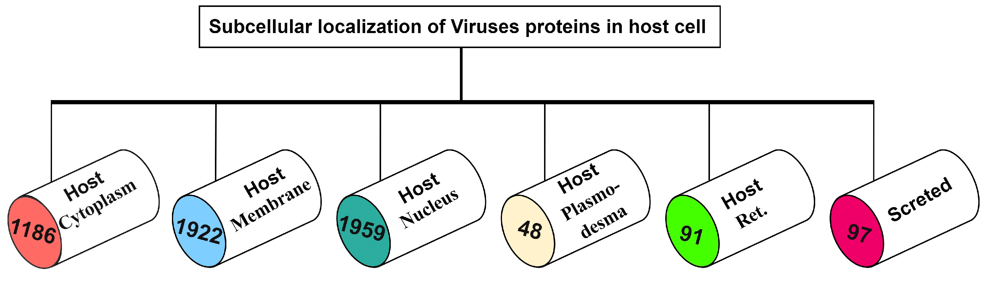
2. Materials and Methods
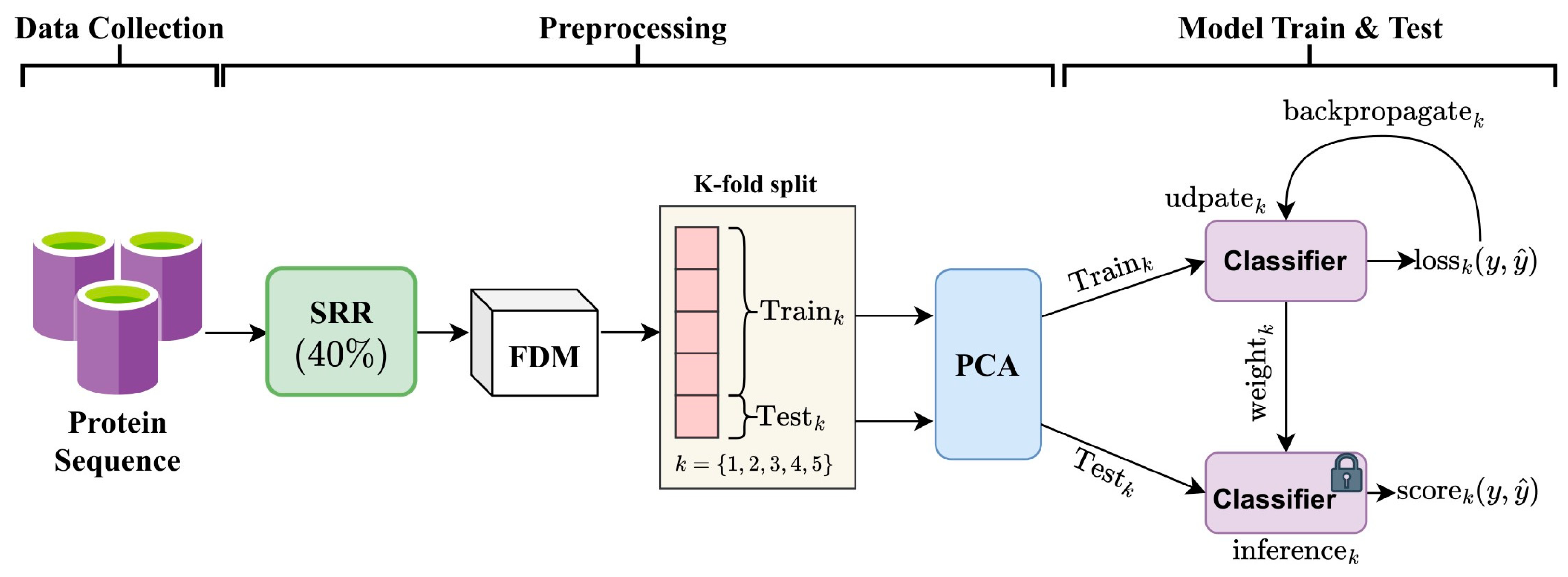
2.1. Framework

High-quality data is the foundation of an excellent model [17,18,19]. In this study, protein sequences were extracted from the Universal Protein Source (UniProt) and underwent several preprocessing stages to ensure data quality, as illustrated in Figure 1. Initially, sequences containing non-standard amino acid characters were removed. Furthermore, the CD-HIT program was employed to eliminate protein sequences with a sequence identity > 40%. Consequently, a high-quality dataset comprising 5303 non-redundant proteins was obtained, as shown in Figure 2. Subsequently, the processed protein sequences underwent feature extraction, and the sequences were converted into numeric feature values based on amino acid composition (AAC), pseudo-amino acid composition (PseAAC), or dipeptide deviation from the expected mean (DDE) descriptors. Principal component analysis (PCA) was applied for dimensionality reduction of the features.
During model testing, we employed 5-fold cross-validation, meaning that 4/5 of the data was used for training, and 1/5 for testing, repeated five times. A fixed random seed was set for K-fold splitting. To train the classifier model, a batch of training data (Traink) was fed into the classifier. The error (loss) was computed and utilized for backpropagation to fine-tune the weights of the model. After iterating through the entire training data with classifier weight updates, we evaluated the learned classifier on the Testk data (inference) and assessed model performance using metrics such as accuracy, F1 score, and sensitivity.

2.2. Data Transformation and Feature Extraction

Transforming protein sequences into vectors is a crucial step in using machine learning for protein prediction [20,21]. Here, we employed the iFeature program to convert protein sequences into three distinct types of protein features: amino acid composition (AAC) [22,23,24], pseudo-amino acid composition (PseAAC), and dipeptide deviation from the expected mean (DDE). These features are capable of capturing essential characteristics of protein sequences, thereby facilitating the construction of subsequent prediction models. In the following sections, these features will be comprehensively described and elaborated.

2.2.1. Amino Acid Composition (AAC)

f t = N ( t ) N ,   t A , B , C , ,   Y ,  
where the frequency f(t) describes the frequency of amino acids t occurring in a protein sequence with length N, while N(t) represents the total number of amino acids in the protein sequence.

2.2.2. Pseudo-Amino Acid Composition (PseAAC)

PseAAC is a powerful descriptor for protein sequence. It could include AAC and contain the correlation of physicochemical properties between two residues. Next, we will provide a detailed introduction to this method. At first, assuming   H 1 o i ,   H 2 o i ,   M o ( i ) represent the original hydrophobicity, hydrophilicity, and side chain masses of the 20 natural amino acids, a standard conversion should be performed. Taking hydrophobicity as an example, its standard conversion can be calculated as shown in Equation (2).
H 1 i = H 1 0 ( i ) 1 20 i = 1 20 H 1 0 i i = 1 20 H 1 0 i 1 20 i = 1 20 H 1 0 i 2 20  
Then, we could use the same formulation to standardize the hydrophilicity and side chain masses. The correlation function of the three properties between two residues, Ri and Rj can be defined as shown in Equation (3). At the same time, the sequence order-correlated factor is formulated as shown in Equation (4).
Θ R i , R j = 1 3 H 1 R i H 1 R j 2 + H 2 R i H 2 R j 2 + M R i M R j 2
θ λ = 1 N λ i = 1 N λ Θ R i , R i + λ
where λ is the integer parameter to be chosen that describes the order of association of amino acids. If using fi as the normalized occurrence frequency of amino acid i in a protein sequence, the PseAAC can be defined as described in Equation (5).
x c = f c r = 1 20 f r + y j = 1 λ θ j ,   1 < c < 20   y θ c 20 r = 1 20 f r + y j = 1 λ θ j ,   21 < c < 20 + λ    
where y is the weighting factor for the sequence-order effect. Here, we selected y = 0.05 in iFeature.

2.2.3. Dipeptide Deviation from Expected Mean (DDE)

Three descriptors, dipeptide composition (Dc), theoretical mean (Tm), and theoretical variance (Tv), have been proposed to formulate protein samples. Based on these three parameters, the DDE can be calculated. The Dc can be obtained first, as shown in Equation (6).
D c r , s = N r s N 1 , r , s A , B , C , , Y
where Dc(r,s) is the dipeptide composition of dipeptide ‘rs’. N is the length of the protein or peptide, and Nrs is the number of dipeptides ‘rs’. Tm(r,s) is the theoretical mean defined in Equation (7).
T m r , s = C r C N × C s C N  
where the first and second amino acids in the given dipeptide ‘rs’ are encoded by Cr and Cs, respectively. CN is the number of possible codons, excluding the three-stop codons. As a final step, DDE(r,s) is calculated as shown in Equation (8).
D D E r , s = D c r , s T m ( r , s ) T v ( r , s )  
where Tv(r,s) is defined as the theoretical variance of the dipeptide ‘rs’.

2.3. Principal Component Analysis (PCA)

Biological data often contain a significant amount of noise or irrelevant information, and high-dimensional data introduce challenges such as the curse of dimensionality. Therefore, to address these issues, we employed PCA for dimensionality reduction [25].
PCA is a widely used multivariate statistical analysis technique designed to reduce the dimensionality of a dataset while preserving its information content. It transforms the data into a new set of uncorrelated variables, known as principal components, that capture the maximum variance in the original data. PCA is commonly employed to decrease the number of variables in a dataset, minimize noise, and enhance the interpretability of results. By applying PCA, we can obtain a reduced-dimensional data representation that retains the most important features and allows for efficient analysis and visualization. In this study, we explored different dimensionality reduction ratios calculated as E′ = ρ × E, where E is the number of features depending on the descriptors (AAC, PseAAC, and DDE) and ρ is the reduced rate.

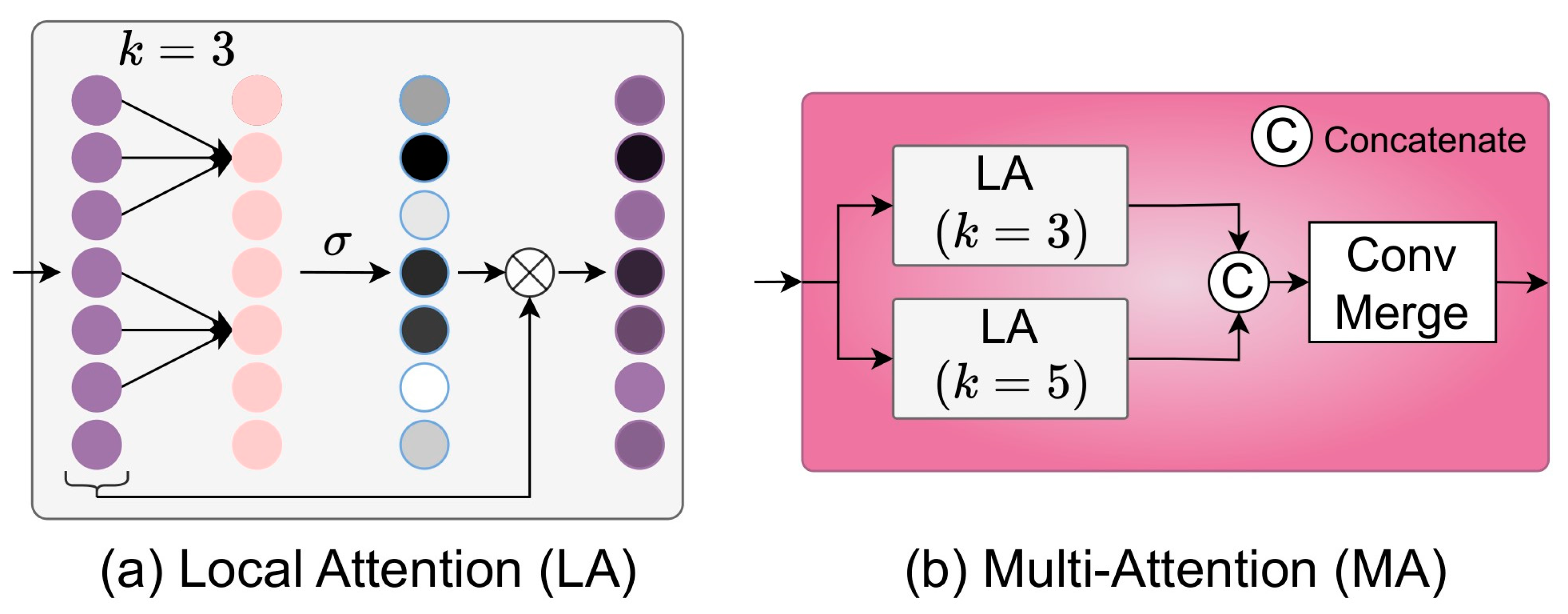
2.4. Ensemble MuLA (E-MuLA) Network

We have proposed an ensemble multi-localized attention (E-MuLA) network for predicting the subcellular localization of viral proteins. Due to feature differences among descriptors (AAC, PseAAC, and DDE), each one yields distinct prediction scores on viral protein subcellular (VPS) sequence data. Hence, we utilize the ensemble technique to improve the prediction performance of our model. The E-MuLA network comprises three descriptor encoders, each receiving a descriptor feature and extracting relevant features. The descriptor encoders in Figure 3 share the same structure, except for differences in the dimension and composition of input features X A C C R E 1 , X P s e A A C R E 2 , X D D E R E 3 . E-MuLA is represented as
E m u l a X A C C , X P s e A A C , X D D E = s o f t m a x   L   U X A C C , X P s e A A C , X D D E ,
where U (·) is a ternary operation, X A C C , X P s e A A C , X D D E are the output descriptor features modeled with their respective encoders {EAAC (·), EPseAAC (·), EDDE (·)}, and L is a linear function with weights {w R 6 × U C , b R 6 }. U C is dependent on the operator in U (·). We employ maximum (M R U C = 64 ), concatenation (C R U C = 64 × 2 ), and summation (S R U C = 64 ) operations in the U (·) to achieve the best accuracy for subcellular localization.

2.4.1. Descriptor Encoder

We have proposed an encoder branch for modeling features of viral protein sequences. As illustrated in Figure 3, there are three encoders, and we focus on detailing one since they share the same architecture. The AAC descriptor encoder is formulated as
X A C C = E A A C ( X A A C )
where E A A C ( . ) R 256   is a descriptor encoder. Each descriptor encoder comprises three feature-extracting blocks and a fully connected network (FCN). A feature-extracting block contains three neural layers: linear, ReLU, and multi-attention. The linear layer is defined as L(X) = wX + b, where w ∈ RC′ × C and b ∈ RC′ are the learnable weight matrix and bias vector, respectively. C′ and C are the output and input features, respectively. We utilize the linear layer to project the input features into high-level features. The rectified linear unit (ReLU) function takes in output from the linear layer and performs non-linear operations on the features using R(X′) = max (0, X′). This helps alleviate the vanishing gradient problem common in training deep neural networks. Finally, the feature-extracting block ends with a multi-attention (MA) module. This module comprises two local attention (LA) modules initialized with varied receptive fields. The receptive fields (k) aid in extracting distinct feature scales from a single input feature, enhancing the output feature. Detailed information about the MA module can be found in Section 2.4.2. After passing the descriptor input feature X through the feature-extracting blocks, the FCN module takes the output and reduces the feature dimension gradually. The FCN is sequentially stacked with linear and ReLU layers. FCN is formulated as F(X) = R(L″(R(L′(X)))) where L′ contains learnable matrices {w R 128×256, b R 128}, and L′′ has learnable matrices {w R 64×128, b R 64}.

2.4.2. Multi-Attention (MA) Module

The multi-attention module comprises multiple local attention modules that utilize different receptive fields (kernel sizes). A large amount of aggregation can be carried out by using various receptive fields. Given the output feature from the previous layer, the local attention module can be formulated as
Χ ~ = σ f w Χ Χ ,  
where σ denotes the Sigmoid function and fw( ) represents the attention function with kernel weight W of the form:
W = w 1,1 0 0 w 2,2 w 1 , k 0 0 w 2 , k + 2 0 0 0 0 w c , c k + 1 0   0 0 w c , c    
The i-th weight of xi can be calculated as
w i = σ j = 1 k w i Χ i j ,   Χ i j Ω i k  
where Ωk represents a set of k neighboring features of xi. This is implemented with a 1D convolution, which is simplified as X ~ = σ C 1 D k X X , where C1D is a 1D convolution function. Using the multiple receptive fields, the multi-attention can be calculated as
Χ = C M σ C 1 D k 1 Χ Χ , σ C 1 D k 2 Χ Χ ,
where k1 = 3, k2 = 5, and CM(.)     RC (conv merge) denotes a 1d convolution function that has learnable weight w   RC×C×2. The visual representation of our local attention and multi-attention modules is shown in Figure 4.

2.5. Other Algorithms

For other machine learning algorithms, we used the Scikit-learn library.

2.5.1. AdaBoost Classifier

The AdaBoost algorithm was originally developed for binary classification, and Hastie et al. extended it to handle multi-classification problems [26]. Its principle is to combine multiple weak classifiers obtained through an iterative process. Each classifier is assigned a weight, and the final AdaBoost model is formulated as a linear combination of these weighted classifiers. In this work, we set the number of estimators to 100.

2.5.2. Decision Trees (DTs)

DT is also a common machine learning method. Each internal node in the decision tree corresponds to an input feature, and each node is labeled with possible target features or sub-decision nodes representing different input features. The tree leaves are labeled with class labels or probability distributions over the classes.

2.5.3. K-Nearest Neighbors (KNNs)

The KNN algorithm assigns each test data to its k-nearest neighbor class. Given the value of k, the label of a data sample is determined by the most common label assigned to its k-nearest training samples. The Euclidean distance is used to measure the proximity between data samples with continuous features.

2.5.4. SGD Classifier

The SGD classifier approximates regularized linear algorithms by using stochastic gradient descent learning. The loss is calculated for each data sample, and the model is updated based on the learning rate. The SGD classifier employs a mini-batch approach, where a subset of the data is fed to the model at each iteration. The linear algorithm used in this classifier is SVM. For this work, we set the number of iterations to 1000.

2.5.5. Gaussian Process Classifier (GPC)

GPCs extend Gaussian Processes used in regression for classification. In this process, functions are modeled as a distribution rather than as a fixed, deterministic function. This can be useful in situations with limited or noisy data. The GPC aims to classify data into multiple classes by inferring decision boundaries based on a Gaussian Process. This is done by assuming data points from each class follow a Gaussian distribution. This approach allows probabilistic decision-making, enhancing classification performance [27].

2.5.6. Linear Support Vector Machine (LSVM)

SVM is a robust and widely used supervised machine learning algorithm for binary classification tasks [28,29,30,31]. It can also be extended to handle multi-class classification problems using techniques such as one-vs-all or one-vs-one. Its principle is to find the most appropriate hyperplane that separates data points of different classes in a high-dimensional feature space. The hyperplane is chosen to maximize the margin between the two types, i.e., the distance between the hyperplane and the closest data points (support vectors) from each category. In this work, we used a linear kernel function in SVM.

2.5.7. Long Short-Term Memory (LSTM) Classifier

The LSTM is a type of recurrent neural network (RNN) architecture that addresses the issues of vanishing and exploding gradients in traditional RNNs [32]. It is particularly effective in processing sequential and time-dependent data [33]. For this study, we constructed a three-layer LSTM network with 32, 64, and 128 output feature dimensions. Following the LSTM layers, we added a fully connected layer with input features of size 128 × 16 to classify the data samples into distinct classes [34].

2.5.8. Convolutional Neural Network (CNN) Classifier

CNN is a widely used and powerful technique in deep learning for classification tasks [35]. CNN utilizes learnable parametric kernels to extract informative feature maps from the input data. In this work, we designed a CNN consisting of three 1D convolutional layers, each followed by a ReLU activation function. The final component of the network is a fully-connected layer that assigns class labels to the input data samples. The output channels for the three convolutional layers were set to 32, 64, and 128, respectively. The fully-connected layer has input features of size 128 × 10.

3. Experimentation

This section discusses the experimental setup and evaluation metrics used for this work.

3.1. Implementation Details

The proposed deep learning methods were implemented using the PyTorch framework and executed on an RTX 2070 GPU. We utilized a batch size of eight for training and evaluation, with a learning rate of 0.0001. The model was trained for 100 epochs to ensure convergence. To assess the generalizability of our models, we employed a 5-fold cross-validation approach in our experiments. The implementation code is available at https://github.com/mercurehg/emula, accessed on 6 March 2024.

3.2. Evaluation Metrics

Additionally, we compared our method with other methods to evaluate its performance. Equation (15) presents the formulation of Precision, Recall, Accuracy, F1, Specificity, Sensitivity, and MCC, which are utilized in this work as evaluation metrics [19,36,37,38,39]. These evaluation metrics play a crucial role in assessing the efficiency and effectiveness of machine learning models. In Equation (15), TP represents the number of true positive predictions (correctly predicted positive subcellular localizations), FP represents the number of false positive predictions (incorrectly predicted positive subcellular localizations), TN represents the number of true negative predictions (correctly predicted negative subcellular localizations), FN represents the number of false negative predictions (incorrectly predicted negative subcellular localizations), and MCC represents Mathew’s correlation coefficient. These metrics provide valuable insights into the accuracy and performance of the subcellular localization predictions.
P r e c i s i o n   ( P r e c ) = T P T P + F P   R e c a l l   ( R e c ) = T P T P + F N   A c c u r a c y   ( A c c ) = T P + T N T P + F P + T N + F N F 1 s c o r e ( F 1 ) = 2 × P r e c i s o n × R e c a l l P r e c i s i o n + R e c a l l   S p e c i f i c i t y   ( S p e c ) = T N T N + F P S e n s i t i v i t y   ( S e n ) = T P T P + F N M C C = T P × T N × F N T P + F N T P + F N T N + F P T N + F N

4. Results and Discussion

We conducted a detailed examination of the performance of the proposed models and compared them with state-of-the-art methods.

4.1. Investigation of PCA

In this study, the performance of each encoding feature (AAC, PseAAC, or DDE) was also examined using 5-fold cross-validation. Firstly, we applied Principal Component Analysis (PCA) to reduce the dimensionality of the three types of feature descriptors. Different reduction rates (ρ) were set for each input feature, and the results were compared, as shown in Table 1. We observed that when the reduction rate reached 0.8, both AAC and PseAAC descriptors showed significant improvements in precision, recall, and F1 scores. In the case of DDE, the optimal results were obtained when the reduction rate reached 0.2. These results indicate that utilizing PCA for dimensionality reduction is effective in eliminating redundant information and noise.
Figure 5 shows the results of 100 epochs for CNN, LSTM, Virus-mPLoc, and MuLA models, displaying both the average performance (line plots) and the corresponding standard deviation (shaded region around the line plots), offering a comprehensive view of the model’s variability. The MuLA network performs better and converges faster than the Virus-mPLoc, LSTM, and CNN deep learning networks for the three descriptors. MuLA networks have lower standard deviation than the other models, which proves MuLA is more consistent and has less variability.

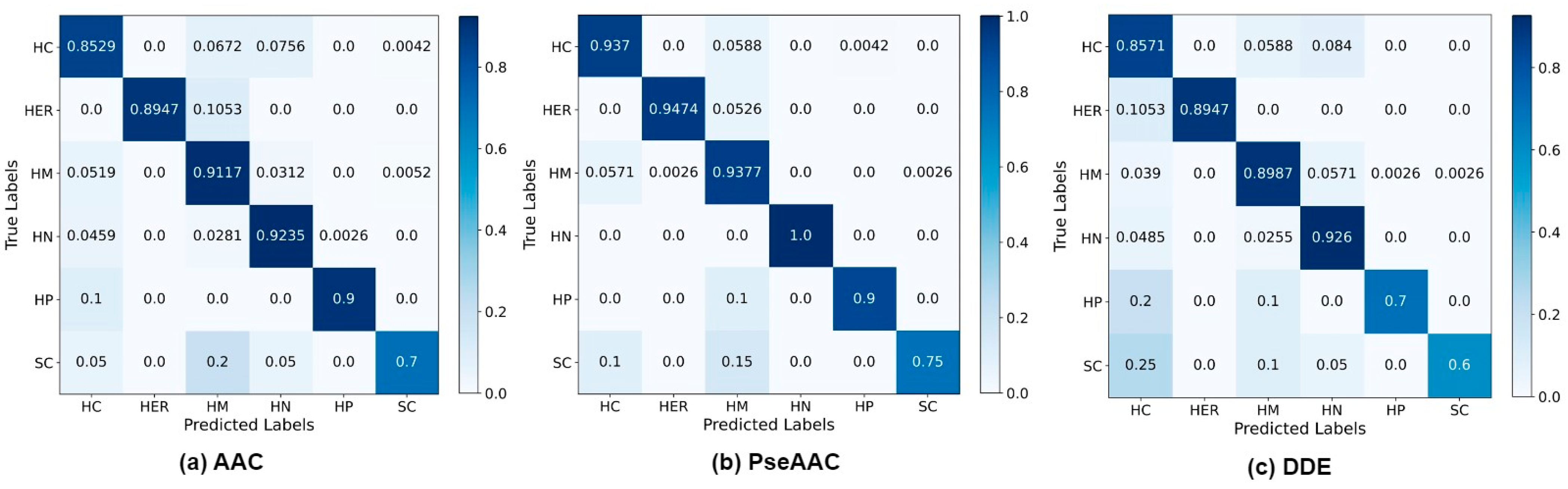
4.2. Investigation of MuLA

We further investigated the impact of multi-attention (MA) in the MuLA model on the performance of multiple descriptors. It was observed that in the absence of MA, the predictive performance of MuLA using AAC, PseAAC, and DDE descriptors decreased, as shown in Table 2. The model performance when using only receptive fields k1 = 3 and k1 = 5 without MA is also documented in Table 2. It can be observed that the results with k1 = 5 surpass those with k1 = 3 for all metrics that utilized AAC, PseAAC, and DDE descriptors. Employing MA with two receptive fields (k1 = 3, k2 = 5) yielded the highest scores for accuracy, precision, recall, F1, and MCC metrics across all descriptors. These results indicate that the correlation of neighboring features in feature descriptors is beneficial for enhancing the predictive capability of the model.
The confusion matrix provides a value description of misclassification rates between subcellular localizations of viral protein. These misclassifications occur because of the similarity of features between samples belonging to different classes and the difficulty of the model in accurately distinguishing these subtle feature differences. Figure 6a–c shows the confusion matrices for the AAC, PseAAC, and DDE descriptors. In these matrices, subcellular localizations are abbreviated as follows: Host Cytoplasm (HC), Host Endoplasmic Reticulum (HER), Host Membrane (HM), Host Nucleus (HN), Host Plasmodesma (HP), and Secreted (SC).
For the AAC descriptor matrix, it is evident that several subcellular localizations are prone to misclassification. For instance, approximately 20% of SC subcellular samples are incorrectly classified as HM, and 5% are misclassified as HC. Similarly, about 10% of HER subcellular samples are misclassified as HM. For the PseAAC descriptor, the misclassification rate is relatively high for HP and SC subcellular localizations. Approximately 20% of HP samples are incorrectly predicted as HN and 16% of SC samples are misclassified as HC. Furthermore, about 15% of SC samples are wrongly classified as HM.

4.3. Comparison with State-of-the-Art Methods

We compared the proposed method with other machine learning methods, deep learning models, and a published model (Virus-mPLoc) to validate the effectiveness of our proposed approach. The results for the AAC descriptor in Table 3 show that the GPC model outperformed the LSTM, CNN, and Virus-mPLoc models in terms of accuracy, precision, recall, F1-score, specificity, sensitivity, and MCC metrics, with values of 86.70%, 84.43%, 77.25%, 80.01%, 96.49%,77.25%, and 80.85%, respectively. Similarly, the KNN model is superior to the LSTM, CNN, and Virus-mPLoc models. As depicted in Table 3, our model performed excellently in all metrics when compared to those of machine learning algorithms, LSTM, CNN and Virus-mPLoc models. For the PseAAC descriptor in Table 3, the GPC classifier outperformed all other MLCs in terms of accuracy, MCC, and specificity, with values of 92.85%, 89.88%, and 97.80%, respectively. Likewise, the GPC classifier outperformed all other MLCs for the DDE descriptor in terms of accuracy, precision, recall, F1-score, specificity, sensitivity, and MCC, achieving values of 85.85%, 86.48%, 77.36%, 80.09%, 95.99%, 77.36%, and 78.98%, respectively. These comparisons demonstrate that MuLA can effectively learn relevant features to distinguish various subcellular sequences of viral proteins.
Given the prediction improvement demonstrated by ensemble networks, we finally evaluated our E-MuLA network using the AAC, PseAAC, and DDE branch encoders. Table 3 includes results of maximum (M), concatenation (C), and summation (S) operations used in the ternary fusion U. E-MuLA performed worse in using C than M. E-MuLA with S outperformed all the other ternary fusion operations. E-MuLA achieved better results than employing a single MuLA network on the individual descriptors.

5. Conclusions

This study introduced the E-MuLA network, a novel deep-learning model that incorporates a multi-attention module to enhance the accuracy of viral protein subcellular localization classification. Through extensive experiments and evaluations, the superiority of the E-MuLA model has been demonstrated. Our research shows the importance of deep-learning models in bioinformatics, particularly in predicting the subcellular localization of viral proteins. The E-MuLA model provides a powerful framework for accurate protein subcellular localization prediction, which will greatly contribute to the development of antiviral therapy and our understanding of the behavior of viral proteins in cells. Future work includes expanding the dataset for training and evaluation as well as exploring the application of the E-MuLA model in other fields of bioinformatics by combining systems biology [40,41,42].

Author Contributions

Conceptualization, C.-B.H. and H.L.; methodology, G.-M.B.K.; software, S.B.Y.; validation, H.Z.; formal analysis, G.-M.B.K., S.G. and S.B.Y.; investigation, H.Z. and B.M.M.; resources, H.Z., L.N. and H.L.; data curation, G.-M.B.K. and H.L.; writing original draft preparation, G.-M.B.K.; writing review and editing, B.M.M., L.N., C.-B.H. and H.L.; visualization, H.Z.; supervision, H.L.; project administration: H.L.; funding acquisition, H.L. All authors have read and agreed to the published version of the manuscript.

Funding

This work was funded by the National Nature Science Foundation of China (62372088).

Institutional Review Board Statement

Not applicable.

Informed Consent Statement

Not applicable.

Data Availability Statement

The datasets analyzed in the current study are available in UniProt. Other data are available upon request to the corresponding author.

Conflicts of Interest

The authors declare no conflicts of interest.

References

  1. Scott, M.S.; Oomen, R.; Thomas, D.Y.; Hallett, M.T. Predicting the subcellular localization of viral proteins within a mammalian host cell. Virol. J. 2006, 3, 24. [Google Scholar] [CrossRef] [PubMed]
  2. Li, J.; Zou, Q.; Yuan, L. A review from biological mapping to computation-based subcellular localization. Mol. Ther. Nucleic Acid 2023, 32, 507–521. [Google Scholar] [CrossRef] [PubMed]
  3. Cheng, H.; Rao, B.; Liu, L.; Cui, L.; Xiao, G.; Su, R.; Wei, L. PepFormer: End-to-End transformer-based siamese network to predict and enhance peptide detectability based on sequence only. Anal. Chem. 2021, 93, 6481–6490. [Google Scholar] [CrossRef] [PubMed]
  4. Shen, H.B.; Chou, K.C. Virus-PLoc: A fusion classifier for predicting the subcellular localization of viral proteins within host and virus-infected cells. Biopolym. Orig. Res. Biomol. 2007, 85, 233–240. [Google Scholar] [CrossRef]
  5. Cao, C.; Shao, M.; Zuo, C.; Kwok, D.; Liu, L.; Ge, Y.; Zhang, Z.; Cui, F.; Chen, M.; Fan, R.; et al. RAVAR: A curated repository for rare variant-trait associations. Nucleic Acids Res. 2024, 52, D990–D997. [Google Scholar] [CrossRef]
  6. Ning, L.; Liu, M.; Gou, Y.; Yang, Y.; He, B.; Huang, J. Development and application of ribonucleic acid therapy strategies against COVID-19. Int. J. Biol. Sci. 2022, 18, 5070–5085. [Google Scholar]
  7. Ren, L.; Ning, L.; Yang, Y.; Yang, T.; Li, X.; Tan, S.; Ge, P.; Li, S.; Luo, N.; Tao, P.; et al. MetaboliteCOVID: A manually curated database of metabolite markers for COVID-19. Comput. Biol. Med. 2023, 167, 107661. [Google Scholar] [CrossRef]
  8. Shen, H.-B.; Chou, K.-C. Virus-mPLoc: A fusion classifier for viral protein subcellular location prediction by incorporating multiple sites. J. Biomol. Struct. Dyn. 2010, 28, 175–186. [Google Scholar] [CrossRef]
  9. Ren, L.; Xu, Y.; Ning, L.; Pan, X.; Li, Y.; Zhao, Q.; Pang, B.; Huang, J.; Deng, K.; Zhang, Y. TCM2COVID: A resource of anti-COVID-19 traditional Chinese medicine with effects and mechanisms. iMETA 2022, 1, e42. [Google Scholar] [CrossRef] [PubMed]
  10. Xiao, X.; Wu, Z.-C.; Chou, K.-C. iLoc-Virus: A multi-label learning classifier for identifying the subcellular localization of virus proteins with both single and multiple sites. J. Theor. Biol. 2011, 284, 42–51. [Google Scholar] [CrossRef] [PubMed]
  11. Li, J.; Zhang, L.C.; He, S.D.; Guo, F.; Zou, Q. SubLocEP: A novel ensemble predictor of subcellular localization of eukaryotic mRNA based on machine learning. Brief. Bioinform. 2021, 22, bbaa401. [Google Scholar] [CrossRef]
  12. Thakur, A.; Rajput, A.; Kumar, M. MSLVP: Prediction of multiple subcellular localization of viral proteins using a support vector machine. Mol. BioSyst. 2016, 12, 2572–2586. [Google Scholar] [CrossRef] [PubMed]
  13. Xiao, X.; Cheng, X.; Chen, G.; Mao, Q.; Chou, K.-C. pLoc_bal-mVirus: Predict subcellular localization of multi-label virus proteins by Chou’s general PseAAC and IHTS treatment to balance training dataset. Med. Chem. 2019, 15, 496–509. [Google Scholar] [CrossRef] [PubMed]
  14. Shao, Y.; Chou, K.-C. pLoc_Deep-mVirus: A CNN model for predicting subcellular localization of virus proteins by deep learning. Nat. Sci. 2020, 12, 388–399. [Google Scholar] [CrossRef]
  15. Ding, Y.J.; Tiwari, P.; Guo, F.; Zou, Q. Shared subspace-based radial basis function neural network for identifying ncRNAs subcellular localization. Neural Netw. 2022, 156, 170–178. [Google Scholar] [CrossRef] [PubMed]
  16. Wang, R.; Jiang, Y.; Jin, J.; Yin, C.; Yu, H.; Wang, F.; Feng, J.; Su, R.; Nakai, K.; Zou, Q. DeepBIO: An automated and interpretable deep-learning platform for high-throughput biological sequence prediction, functional annotation and visualization analysis. Nucleic Acids Res. 2023, 51, 3017–3029. [Google Scholar] [CrossRef] [PubMed]
  17. Zhang, Y.; Pan, X.; Shi, T.; Gu, Z.; Yang, Z.; Liu, M.; Xu, Y.; Yang, Y.; Ren, L.; Song, X.; et al. P450Rdb: A manually curated database of reactions catalyzed by cytochrome P450 enzymes. J. Adv. Res. 2023, in press. [Google Scholar] [CrossRef] [PubMed]
  18. Wu, S.; Feng, J.; Liu, C.; Wu, H.; Qiu, Z.; Ge, J.; Sun, S.; Hong, X.; Li, Y.; Wang, X.; et al. Machine learning aided construction of the quorum sensing communication network for human gut microbiota. Nat. Commun. 2022, 13, 3079. [Google Scholar] [CrossRef]
  19. Tang, Y.; Pang, Y.; Liu, B. IDP-Seq2Seq: Identification of intrinsically disordered regions based on sequence to sequence learning. Bioinformatics 2021, 36, 5177–5186. [Google Scholar] [CrossRef]
  20. Pham, N.T.; Phan, L.T.; Seo, J.; Kim, Y.; Song, M.; Lee, S.; Jeon, Y.J.; Manavalan, B. Advancing the accuracy of SARS-CoV-2 phosphorylation site detection via meta-learning approach. Brief. Bioinform. 2023, 25, bbad433. [Google Scholar] [CrossRef]
  21. Pham, N.T.; Rakkiyapan, R.; Park, J.; Malik, A.; Manavalan, B. H2Opred: A robust and efficient hybrid deep learning model for predicting 2’-O-methylation sites in human RNA. Brief. Bioinform. 2023, 25, bbad476. [Google Scholar] [CrossRef]
  22. Zhu, W.; Yuan, S.S.; Li, J.; Huang, C.B.; Lin, H.; Liao, B. A First Computational Frame for Recognizing Heparin-Binding Protein. Diagnostics 2023, 13, 2465. [Google Scholar] [CrossRef]
  23. Zou, X.; Ren, L.; Cai, P.; Zhang, Y.; Ding, H.; Deng, K.; Yu, X.; Lin, H.; Huang, C. Accurately identifying hemagglutinin using sequence information and machine learning methods. Front. Med. 2023, 10, 1281880. [Google Scholar] [CrossRef]
  24. Li, H.; Pang, Y.; Liu, B. BioSeq-BLM: A platform for analyzing DNA, RNA, and protein sequences based on biological language models. Nucleic Acids Res. 2021, 49, e129. [Google Scholar] [CrossRef] [PubMed]
  25. Sun, B.; Chen, S.; Wang, J.; Chen, H. A robust multi-class AdaBoost algorithm for mislabeled noisy data. Knowl.-Based Syst. 2016, 102, 87–102. [Google Scholar] [CrossRef]
  26. Hastie, T.; Rosset, S.; Zhu, J.; Zou, H. Multi-class adaboost. Stat. Its Interface 2009, 2, 349–360. [Google Scholar] [CrossRef]
  27. MacKay, D.J. Introduction to Gaussian processes. NATO ASI Ser. F Comput. Syst. Sci. 1998, 168, 133–166. [Google Scholar]
  28. Wang, Y.; Zhai, Y.; Ding, Y.; Zou, Q. SBSM-Pro: Support Bio-sequence Machine for Proteins. arXiv 2023, arXiv:2308.10275. [Google Scholar]
  29. Zhang, H.Y.; Zou, Q.; Ju, Y.; Song, C.G.; Chen, D. Distance-based Support Vector Machine to Predict DNA N6-methyladenine Modification. Curr. Bioinform. 2022, 17, 473–482. [Google Scholar] [CrossRef]
  30. Liu, B.; Gao, X.; Zhang, H. BioSeq-Analysis2.0: An updated platform for analyzing DNA, RNA and protein sequences at sequence level and residue level based on machine learning approaches. Nucleic Acids Res. 2019, 47, e127. [Google Scholar] [CrossRef]
  31. Ao, C.; Ye, X.; Sakurai, T.; Zou, Q.; Yu, L. m5U-SVM: Identification of RNA 5-methyluridine modification sites based on multi-view features of physicochemical features and distributed representation. BMC Biol. 2023, 21, 93. [Google Scholar] [CrossRef] [PubMed]
  32. Muhuri, P.S.; Chatterjee, P.; Yuan, X.; Roy, K.; Esterline, A. Using a long short-term memory recurrent neural network (LSTM-RNN) to classify network attacks. Information 2020, 11, 243. [Google Scholar] [CrossRef]
  33. Chen, J.; Zou, Q.; Li, J. DeepM6ASeq-EL: Prediction of Human N6-Methyladenosine (m6A) Sites with LSTM and Ensemble Learning. Front. Comput. Sci. 2022, 16, 162302. [Google Scholar] [CrossRef]
  34. Tang, Y. Deep learning using linear support vector machines. arXiv 2013, arXiv:1306.0239. [Google Scholar]
  35. Zou, Q.; Xing, P.; Wei, L.; Liu, B. Gene2vec: Gene Subsequence Embedding for Prediction of Mammalian N6-Methyladenosine Sites from mRNA. RNA 2019, 25, 205–218. [Google Scholar] [CrossRef]
  36. Zulfiqar, H.; Guo, Z.; Ahmad, R.M.; Ahmed, Z.; Cai, P.; Chen, X.; Zhang, Y.; Lin, H.; Shi, Z. Deep-STP: A deep learning-based approach to predict snake toxin proteins by using word embeddings. Front. Med. 2024, 10, 1291352. [Google Scholar] [CrossRef] [PubMed]
  37. Zhu, H.; Hao, H.; Yu, L. Identifying disease-related microbes based on multi-scale variational graph autoencoder embedding Wasserstein distance. BMC Biol. 2023, 21, 294. [Google Scholar] [CrossRef]
  38. Hasan, M.M.; Tsukiyama, S.; Cho, J.Y.; Kurata, H.; Alam, M.A.; Liu, X.; Manavalan, B.; Deng, H.W. Deepm5C: A deep-learning-based hybrid framework for identifying human RNA N5-methylcytosine sites using a stacking strategy. Mol. Ther. 2022, 30, 2856–2867. [Google Scholar] [CrossRef]
  39. Bupi, N.; Sangaraju, V.K.; Phan, L.T.; Lal, A.; Vo, T.T.B.; Ho, P.T.; Qureshi, M.A.; Tabassum, M.; Lee, S.; Manavalan, B. An Effective Integrated Machine Learning Framework for Identifying Severity of Tomato Yellow Leaf Curl Virus and Their Experimental Validation. Research 2023, 6, 0016. [Google Scholar] [CrossRef]
  40. Manavalan, B.; Patra, M.C. MLCPP 2.0: An Updated Cell-penetrating Peptides and Their Uptake Efficiency Predictor. J. Mol. Biol. 2022, 434, 167604. [Google Scholar] [CrossRef]
  41. Shoombuatong, W.; Basith, S.; Pitti, T.; Lee, G.; Manavalan, B. THRONE: A New Approach for Accurate Prediction of Human RNA N7-Methylguanosine Sites. J. Mol. Biol. 2022, 434, 167549. [Google Scholar] [CrossRef] [PubMed]
  42. Thi Phan, L.; Woo Park, H.; Pitti, T.; Madhavan, T.; Jeon, Y.J.; Manavalan, B. MLACP 2.0: An updated machine learning tool for anticancer peptide prediction. Comput. Struct. Biotechnol. J. 2022, 20, 4473–4480. [Google Scholar] [CrossRef] [PubMed]
Figure 1. The illustrative flow of the framework for training and testing learning classifiers for predicting viral protein subcellular.
Information 15 00163 g001
Figure 2. Groupings of Viruses Proteins in the host cell and number of samples for each group.
Information 15 00163 g002
Figure 3. Illustration of our proposed Ensemble MuLA (E-MuLA) network.
Information 15 00163 g003
Figure 4. Schematic representation of proposed (a) local attention (LA) and (b) multi-attention (MA) modules.
Information 15 00163 g004
Figure 5. Average and standard deviation results of MuLA (Ours), CNN, LSTM, and Virus-mPLoc during training.
Information 15 00163 g005
Figure 6. The visualization of misclassification of subcellular localization categories for AAC, PseAAC, and DDE descriptors.
Information 15 00163 g006
Table 1. The results of different numbers of PCA components.
Rat (ρ) AAC PseAAC DDE
AccPrecRecF1MCCAccPrecRecF1MCCAccPrecRecF1MCC
0.274.6071.8365.3366.8762.6290.0980.7272.1574.185.4586.3387.9378.1981.9479.89
0.484.5580.9175.8377.3977.3292.5585.578.6480.7489.0782.7782.8874.3977.5474.64
0.686.9884.4678.5480.6780.8593.5988.180.7983.2190.680.6481.7171.8275.3771.47
0.887.7186.5579.5382.1681.9294.0088.6682.284.1791.2179.1581.3569.5573.7169.22
1.087.6285.7279.4081.7481.8093.9488.1281.3883.6291.1274.5676.3265.5769.4462.43
Table 2. Performance comparison of MuLA model with (w) and without (w/o) multi-attention (MA) with receptive fields (k1 = 3, k2 = 5).
MAAACPseAACDDE
AccMCCAccMCCAccMCC
w/o84.1379.6593.0190.2280.7473.89
w (k1 = 3)85.4380.1193.7490.8382.6374.44
w (k2 = 5)86.7280.4693.8490.9884.4777.15
w (k1 = 3, k2 = 5)87.7181.9294.0091.2186.3379.89
Table 3. Classification report on AAC, PseAAC, and DDE descriptors and comparison against baselines.
ModelAccPrecRecF1SpecSenMCC
AAC (Only)
AdaBoost38.0428.8832.225.6186.9632.220.61
DT78.4968.6169.7568.8494.8269.7568.48
KNN84.1681.1771.3573.9596.2171.3576.83
GPC86.784.4377.2580.0196.4977.2580.85
LSVM69.7348.9344.0445.3292.3344.0454.69
SGD64.8144.0334.6535.4491.1134.6547.21
LSTM63.7541.9340.7440.5790.8740.7445.73
CNN62.8338.6636.0635.8490.4936.0644.14
Virus-mPLoc [8]65.6342.1339.2939.5791.3339.2948.41
MuLA87.7186.5579.5382.1697.079.5381.92
PseACC (only)
AdaBoost51.1521.2423.3918.9588.2623.3931.67
DT89.3173.5175.6573.5197.675.6584.36
KNN92.7484.1480.180.4997.3680.189.4
GPC92.8587.0681.1982.5997.881.1989.88
LSVM86.3758.4855.5456.5796.7455.5479.8
SGD84.4155.9348.3849.5196.2848.3876.92
LSTM80.9250.3148.7748.5595.3848.7772.03
CNN82.7251.6548.1948.3495.7148.1974.94
Virus-mPLoc [8]81.2147.1345.2545.195.3845.2572.37
MuLA94.088.6682.284.1798.6182.291.21
DDE (only)
AdaBoost48.0640.8832.8431.1887.0632.8425.24
DT77.6769.1568.0968.1194.6168.0967.25
KNN84.8684.0976.6279.7695.3676.6277.78
GPC85.8586.4877.3680.0995.9977.3678.98
LSVM79.4677.6862.5466.2494.9262.5469.53
SGD73.5669.4960.2763.7193.5260.2760.92
LSTM60.5242.138.9539.2290.038.9540.68
CNN58.0637.6833.7633.7689.3133.7637.15
Virus-mPLoc [8]57.2736.5632.4132.5389.1532.4135.57
MuLA86.3387.9378.1881.9496.6578.1879.89
Ensemble (AAC, PseAAC, and DDE) with the ternary operators U (·) = {M, C, S} to merge the descriptors features.
E-MuLA (M = maximum)94.7292.3184.1587.3998.7884.1592.26
E-MuLA (C = concatenate)94.5591.5683.8386.8498.7483.8392.01
E-MuLA (S = summation)94.8792.7284.1887.6198.8184.1892.47
Disclaimer/Publisher’s Note: The statements, opinions and data contained in all publications are solely those of the individual author(s) and contributor(s) and not of MDPI and/or the editor(s). MDPI and/or the editor(s) disclaim responsibility for any injury to people or property resulting from any ideas, methods, instructions or products referred to in the content.

