Article

Explainable Machine Learning for Malware Detection on Android Applications †

1
ISEL, Instituto Superior de Engenharia de Lisboa, Instituto Politécnico de Lisboa, 1959-007 Lisboa, Portugal
2
Instituto de Telecomunicações, 1049-001 Lisboa, Portugal
3
IST, Instituto Superior Técnico, Universidade de Lisboa, 1049-001 Lisboa, Portugal
*
Author to whom correspondence should be addressed.
This paper is an extended version of our paper published in 14th Simpósio de Informática (INForum), Porto, Portugal, 7–8 September 2023.
Information 2024, 15(1), 25; https://doi.org/10.3390/info15010025
Submission received: 9 November 2023 / Revised: 29 December 2023 / Accepted: 30 December 2023 / Published: 1 January 2024
(This article belongs to the Special Issue Digital Privacy and Security)

Abstract

:
The presence of malicious software (malware), for example, in Android applications (apps), has harmful or irreparable consequences to the user and/or the device. Despite the protections app stores provide to avoid malware, it keeps growing in sophistication and diffusion. In this paper, we explore the use of machine learning (ML) techniques to detect malware in Android apps. The focus is on the study of different data pre-processing, dimensionality reduction, and classification techniques, assessing the generalization ability of the learned models using public domain datasets and specifically developed apps. We find that the classifiers that achieve better performance for this task are support vector machines (SVM) and random forests (RF). We emphasize the use of feature selection (FS) techniques to reduce the data dimensionality and to identify the most relevant features in Android malware classification, leading to explainability on this task. Our approach can identify the most relevant features to classify an app as malware. Namely, we conclude that permissions play a prominent role in Android malware detection. The proposed approach reduces the data dimensionality while achieving high accuracy in identifying malware in Android apps.

1. Introduction

The worldwide use of smartphones has grown exponentially over the past decade. As of November 2023, the estimated number of smartphone users is 5.25 billion, and it continues to grow [1]. This growth has been accompanied by the popularization of Android, an open-source operating system (OS) mainly designed for touchscreen mobile devices. It is the mobile OS with the largest market share, with roughly 70% [2]. In November 2023, the app store Google Play Store had 3.718 million apps available for Android users to download [3].
The rapid wide-scale expansion of the use of smartphone devices, the increased popularity of the Android OS, and the wide variety and number of Android apps have attracted the attention of malware developers. Attackers can target a wide range of applications that deal with a significant number of user-sensitive data. They can also target the user’s data on the smartphone or may use the device to carry out other attacks. Furthermore, from the attacker’s perspective, the massive number of users are all targets and potential victims who can download their malware. Since the Android system has become a popular and profitable target, malicious attacks against Android mobile devices have increased. In 2021, 9.5 million malware Android packages were detected, three times more than in 2019 (3.1 million) [4]. Millions of users can download one app (possibly with malicious software) in a matter of minutes. Thus, the need to detect malicious apps is a major issue.
Some software and applications focus on security, and app stores have security and detection mechanisms to mitigate malicious apps. To some extent, these are successful, but malware keeps growing in sophistication and diffusion, sometimes easily bypassing these mechanisms. ML approaches have shown to be effective and versatile in various fields, being a milestone in the tech industry. Thus, in recent years, ML techniques have been proposed for the malware detection problem in Android applications [4,5,6,7,8,9,10].

Paper Contributions

This work focuses on the use of ML techniques for malware detection in Android applications, and its main contributions are the following:
  • Assessing the impact of different data pre-processing techniques using four different datasets. Data pre-processing is an essential step and, to the best of our knowledge, this aspect is lacking attention in the literature on this problem.
  • Enriching the literature by identifying the most decisive features for malware detection among the public-domain datasets used and identifying the ML classifiers that provide the best results.
  • Expanding the literature by using real-world Android applications (developed and existing) to extend test scenarios over the ones made available by the datasets. To the best of our knowledge, no previous work has developed specific applications for malware model testing.
In this paper, we extend our previous work [11] with (non-deep) machine learning techniques, providing the following novel contributions and extensions:
  • The use of real-world apps in the assessment of the ML model learned from standard datasets. We also provide a discussion on the challenges posed by the mapping from the real-world app to our learned models.
  • The use of more datasets, feature selection filters, classifiers, and data pre-processing techniques, namely, different instance (numerosity) sampling techniques. The combination of these techniques on an ML pipeline is addressed and evaluated.
  • A detailed and deeper discussion of the experimental results on four datasets instead of two. These four datasets have different characteristics regarding the key aspects of the data. This leads to the need to analyze the results from each dataset individually.
  • For each dataset, we report the top five features that seem to be more decisive regarding malware classification, yielding some explainability on the classification. We highlight the features that most contribute to explaining the classification.
The remainder of this paper is organized as follows. Section 2 provides an overview of Android apps and related work. The proposed approach is described in Section 3. The experimental evaluation is reported in Section 4. Finally, Section 5 ends the paper with concluding remarks and directions for future work.

2. Related Work

This section briefly overviews Android malware detection, approaching ML techniques, algorithms, and datasets. It begins with a general Android app overview in Section 2.1 and malware types and security measures in Section 2.2. Then, it discusses data acquisition, namely, analysis types, and datasets in Section 2.3 and explores techniques for data pre-processing and splitting in Section 2.4. ML algorithms and their evaluation metrics are presented in Section 2.5 and Section 2.6, respectively. This section ends by summarizing previous approaches to malware detection that have been proposed in the literature, in Section 2.7 and Section 2.8.

2.1. Android Applications

Android is an open-source OS based on the Linux kernel, designed mainly for touchscreen mobile devices. First launched in 2008, it has many versions, with releases every few months. To understand how malware can exploit the Android OS, it is essential to know the key components of an Android app. Figure 1 depicts the elements that compose the Android package kit (APK) file of an Android app [10].
Knowledge about the structure of an Android app allows for a better understanding of some of the critical security aspects. For instance, apps require system permissions to perform specific functionalities. Malware often exploits these accesses and permissions to perform attacks [12]. Thus, the AndroidManifest.xml file, with the permissions requested by the app, is relevant in determining if an app is malicious, as discussed in Section 2.3.

2.2. Malware on Android Applications

Malware takes different forms and approaches, such as remote access trojans, banking trojans, ransomware, adware, spyware, scareware, and premium text short message service (SMS). Malware exploits system vulnerabilities, design weaknesses, and security flaws in many Android applications that threaten end-users and/or lure the user through social engineering to install apps containing malware [13]. There are well-documented Android malware families, such as “ExpensiveWal”, “HummingBad”, and “Chamoi”, which can be embedded or hidden in many apps available in app stores and then downloaded by millions of users.
There are several security measures to mitigate malware attacks, such as using secure internet connections, installing anti-malware apps, and the validation of the apps performed by the app stores. Android also inherits some security measures since the kernel provides application sandboxing and process isolation [12]. These security measures, to some extent, successfully mitigate malware attacks. However, sometimes they can be bypassed with a variety of techniques to hinder the identification and neutralization of malware [9].

2.3. Data Acquisition

This section provides insight into the different types of analysis used to extract features from Android apps and into some of the datasets for Android malware detection found in the literature.

2.3.1. Type of Analysis

Three types of approaches can be followed to extract features from Android apps: static, dynamic, and hybrid. Static analysis is the most popular, followed by the dynamic and hybrid approaches [10]. In static analysis, the app is analyzed in a non-runtime environment. Feature extraction is usually carried out by analyzing the code and the AndroidManifest.xml file [9]. It is generally faster and more straightforward than the other analysis types. Dynamic analysis occurs during the app’s regular operation in a monitored, controlled, or sandbox environment [10] to analyze its behavior. Thus, it is computationally more demanding than static analysis [12]. Features can be extracted by analyzing network traffic, system calls, system resources, and other app behaviors [9]. Finally, hybrid analysis combines the previous two types of analysis [12]. However, as with dynamic analysis, researchers are discouraged by the time and computational resources it requires and its complexity, making it the less popular type of analysis.

2.3.2. Datasets

Several standard datasets for malware detection in Android apps are mentioned in the literature [10]. Unfortunately, frequently these are not easy to obtain. Often, the access is restricted, involving payment or authorization. In other cases, the sources may not be trustworthy.
Alkahtani and Aldhyani considered the Drebin and CICAndMal2017 datasets in their study [4], available in [14,15], respectively. The Drebin dataset, first published in 2014, contains 215 features extracted from 15,036 applications, with 9476 benign apps and 5560 malware apps from 179 different malware families. The CICAndMal2017 dataset, published in 2018, contains 183 features and 29,999 instances extracted from several sources, such as the Google Play Store. The malware samples can be organized into adware, ransomware, scareware, and SMS malware, from a total of 42 unique malware families.
The Android Malware (AM) and the Android Malware static feature (AMSF) datasets, available in [16,17], respectively, are also considered in this paper. The AM dataset was created by Martín et al. in 2016, in the context of their study [8]. It contains meta information on Android apps with 183 features and 11,476 instances. The AMSF dataset is organized into six parts, each with different features: permissions, intents, system commands, application programming interface (API) calls, API packages, and opcodes. These datasets were extracted from the same APK. In total, it contains 1062 features and 5019 samples of apps collected from the Google Play Store, APKPure, and VirusShare.

2.4. Data Pre-Processing and Splitting

This section overviews some data pre-processing and data-splitting techniques.

2.4.1. Data Pre-Processing

Data pre-processing can be generalized and aggregated into four categories [18]: cleaning, integration, reduction, and transformation. Data cleaning includes handling missing values, which can be done with different approaches, such as discarding instances with missing values or performing missing value imputation. It also addresses reformatting the data to ensure standard formats and attribute conversions, such as one-hot or label encoding. Data cleaning includes the identification of outliers and the smoothing of noisy data. Data integration consists of merging data from multiple sources into a single dataset. Data reduction techniques aim to derive a reduced representation in terms of volume, keeping the integrity of the original data. The main strategies for data reduction are dimensionality reduction, and numerosity reduction, which includes instance sampling. Dimensionality reduction can be performed by feature selection techniques, such as the relevance-redundancy feature selection(RRFS) filter approach [19]. RRFS involves discarding the weakly relevant and redundant features while keeping the relevant ones adding more value to the model. For relevance analysis, different measures can be applied, such as the unsupervised mean–median (MM) relevance measure given by
M M i = | X i ¯ m e d i a n ( X i ) | ,
with X i ¯ denoting the sample mean of feature X i . We also consider the supervised Fisher’s ratio (FR) relevance metric
F R i = X ¯ i ( 1 ) X ¯ i ( 1 ) var ( X i ) ( 1 ) + var ( X i ) ( 1 ) ,
where X ¯ i ( 1 ) , X ¯ i ( 1 ) , var ( X i ) ( 1 ) , and var ( X i ) ( 1 ) are the sample means and variances of feature X i , for the patterns of each class. The redundancy analysis between two features, X i and X j , is done with the absolute cosine (AC)
A C X i , X j = | c o s ( θ X i X j ) | = | X i , X j | | X i | | | | X j | | | = k = 1 n X i k X j k k = 1 n X i k 2 k = 1 n X j k 2 ,
where , and | | . | | denote the inner product and L 2 norm, respectively.
Numerosity reduction includes instance sampling, a method that balances imbalanced data. Undersampling consists of removing samples of the majority class, yielding information loss. To balance data, oversampling, which involves replicating instances of the minority class, can also be applied, yielding a higher chance of overfitting. Other techniques, such as the synthetic minority oversampling technique (SMOTE) [20], perform oversampling by creating synthetic data instead of copying existing instances.
Lastly, data transformation aims to change the data’s value, structure, or format to shape it into an appropriate form. The most widely used techniques are normalization and discretization. The first involves scaling attributes to ensure they fit within a specified range. One of the most popular techniques for this task is min–max normalization. The use of discretization techniques reduces the number of continuous feature values by partitioning the feature range into intervals to replace the actual data values. The original feature values are replaced by integer indexes that represent each discretization interval, achieving a simplified representation of the data.

2.4.2. Data Splitting

Data are typically split into two or three sets: training, testing, and validation, based on random or stratified sampling. Cross-validation (CV) [21] is a resampling method that splits the data into subsets and rotates their use among them. The nested CV strategy is applied to the training, testing, and validation sets. It consists of an outer loop and an inner loop. The outer loop deals with the training and testing sets and estimates the generalization error by averaging test set scores over several dataset splits. The inner loop deals with the training and validation sets, with all subsets being obtained from the training set of the outer loop. In the inner loop, the score is approximately maximized by fitting a model to each training set and then directly maximized by selecting hyperparameters over the validation set. There are different types of CV, such as stratified K-fold CV and leave-one-out cross-validation (LOOCV). Stratified K-fold CV splits the data into K folds of approximately equal size with stratified sampling. LOOCV is the exhaustive holdout splitting approach, being a particular case of K-fold CV where K is equal to the number of instances.

2.5. Classifiers

In this section, a brief description of the classifiers used in this research is presented. Random forests(RF) [22] is an ensemble method that aggregates the output of multiple decision trees (DT) [23,24] to reach a single result. Support vector machines (SVM) [25] work by mapping data to a high-dimensional feature space to categorize data points. Even when the classes are not linearly separable, the data are transformed so that the separator can be drawn as a hyperplane that best splits the data into two classes [26]. K-nearest neighbors (KNN) [24,27] classifies a data point by a majority vote of its neighbors, with the data point being assigned to the class most common among its K nearest neighbors. Naïve Bayes (NB) classifiers follow a probabilistic approach based on Bayes’ Theorem that relies on incorporating prior probability distributions to generate posterior probabilities [24,28].
As an additional technique, we also consider a classic multilayer perceptron(MLP) [29,30] as a classifier. An MLP has the advantage of learning non-linear models; the ability to train models in real-time (online learning); handling large numbers of input data; and, once trained, making quick predictions. However, it is more computationally costly than other classifiers and may be sensitive to feature scaling. We use the default implementation of MLP from the scikit-learn library, without resorting to deep learning techniques implementations.

2.6. Evaluation Metrics

This section describes the evaluation metrics used to assess the performance of the ML models. In this study, we adopt the following terminology: a true positive (TP) means to classify a malicious app as malicious correctly, a true negative (TN) is to classify a benign app as benign, a false positive (FP) is to classify a benign app as malicious, and a false negative (FN) refers to classifying a malicious app as benign. The accuracy (Acc) evaluation metric conveys the fraction of correct predictions made by the model and is given by
Acc = TP + TN TP + TN + FP + FN .
In very unbalanced scenarios, accuracy can be misleading and other evaluation metrics are used. The positive predictive value, or precision (Prec), is given by
Prec = TP TP + FP ,
whereas the true positive rate (TPR), or sensitivity, also known as recall (Rec), is computed as
Rec = TP TP + FN .
Finally, the F1-score, given by the harmonic mean of the precision and recall metrics
F 1 = 2 Precision × Rec Precision + Rec ,
is also considered, as well as the area under the curve—receiver operating characteristic (AUC-ROC) evaluation metric is also considered.

2.7. Overview of Machine Learning Approaches

This section focuses on the use of some common ML approaches for Android malware detection found in the literature. Section 2.8 addresses other techniques such as deep learning (DL).
Alkahtani and Aldhyani [4] applied SVM and KNN to two standard datasets: CICAndMal2017 and Drebin. SVM achieved an 80.71% accuracy with the Drebin dataset. For the CICAndMal2017 dataset, the authors claim to have achieved 100% accuracy. Regarding KNN, it achieved 81.57% on the Drebin dataset and 90% on the CICAndMal2017 dataset. Overall, SVM and KNN successfully detected malware, but SVM was more effective.
Muzaffar et al. [12] identified that many existent studies cite high accuracy rates. However, many use outdated datasets and inappropriate evaluation metrics that may be misleading. Kouliaridis and Kambourakis [9] concluded that, among the surveyed works, static analysis is the predominant approach, while publicly available datasets are often outdated. ML-based models are the most commonly used, and accuracy is the preferred evaluation metric. In studies from 2014 to 2021, RF and SVM are the most frequently employed algorithms. Wu et al. [10] provided insight into the most popular datasets used in the literature and concluded that the most used ML algorithms for Android malware detection between 2019 and 2020 were SVM, RF, and KNN.
Keyvanpour et al. [7] conducted experiments with the Drebin dataset and proposed embedding effective FS with RF. Other classifiers, such as KNN and NB, were tested, but RF outperformed other models based on several metrics. FS was shown to improve the RF classifier, with the authors reporting 99.49% accuracy and AUC of 95.6%, when using effective FS and RF with 100 trees.
Islam et al. [6] used the CCCS-CIC-AndMal2020 dataset, with 53,439 instances and 141 features. Missing data imputation was applied with the “mean” strategy, and SMOTE was used to deal with class imbalance. Min–max normalization was applied, and one-hot encoding was used for feature conversion. Recursive feature elimination (RFE) was used to perform FS, discarding 60.2% of the features. The reduced set of features lessened the complexity and improved the accuracy. The authors proposed multi-classification based on dynamic analysis, with an ensemble ML approach with weighted voting that incorporates RF, KNN, MLP, DT, SVM, and logistic regression (LR), which showed 95% accuracy.
Alomari et al. [31] proposed a multi-classification approach using the CICMalDroid2020 dataset, with 11,598 instances and 470 features. The z-score normalization, SMOTE and principal component analysis (PCA), were applied. SMOTE and z-score normalization improved the results, while PCA was not beneficial. Their approach was based on the light gradient boosting mode (LightGBM), but the performance of KNN, RF, DT, and NB was also analyzed. LightGBM presented the best accuracy and F1-score, achieving 95.49% and 95.47%, respectively.
Kouliaridis et al. [32] review the literature on Android malware detection, spanning the period from 2012 to 2020. On the Drebin, VirusShare, and AndroZoo datasets, the authors rank the importance of features with the Information Gain metric. They found that features related to permissions and intents rank higher than others. However, the single use of permission-related features alone, and the mixture of permission- and intent-related features, does not yield remarkable results in malware detection. Thus, the authors identify the need to check supplementary and more weighty features.
In another work by Kouliaridis et al. [33], the authors explore the use of the dimensionality reduction techniques PCA and t-SNE (t-distributed stochastic neighbor embedding) in malware detection. The authors propose a simple ensemble aggregated base model of similar feature types and a complex ensemble with heterogeneous base models. The experimental results on the Androzoo dataset show the adequacy of ensembles for malware detection.
The Androtomist tool for the static and dynamic analysis of applications on the Android platform is proposed by Kouliaridis et al. in [34]. This hybrid approach resorts to features stemming from static analysis along with dynamic instrumentation. The approach resorts to machine learning and signature-based detection techniques. Androtomist software is made publicly available as open source and can be installed as a web application. The authors also provide an ensemble approach with an insight on the most influencing features regarding the classification process. The approach shows promising to excellent results in terms of the accuracy, F1-score, and AUC-ROC metrics.
Potha et al. [35] find that heterogeneous ensembles can provide malware detection solutions that are better than individual models. They propose the extrinsic random-based ensemble (ERBE) method, which uses a given set of repetitions and a subset of external (malware or benign) instances. The classification features are randomly selected, and an aggregation function combines the output of all base models for each test case separately. Using solely static analysis, the ERBE method takes advantage of the availability of multiple external instances of different sizes and genres. The experimental results with the AndroZoo dataset show the effectiveness of the proposed method.
Table 1 summarizes some results reported in the existing approaches.

2.8. Other Approaches and Surveys on the Topic

There are other approaches to detecting malware in Android apps. For example, the use of deep learning (DL) techniques has provided satisfactory results, as reported in the works by [4,10,31,36,37,38], in relation to detecting malware on Android apps.
An ML approach with data from the Canadian Institute for Cybersecurity is reported by Akhtar and Feng [39], showing that DT, SVM, and convolutional neural networks (CNNs) performed well, with DT being the best classifier. A hybridization of CNN and ML techniques is proposed by Hashin in [40].
The work by Djenna et al. [41] addresses the combination of behavior-based deep learning and heuristic-based approaches for malware detection, comparing them with static deep learning methods. Online learning has also been proposed by Muzaffar et al. [12]. Shaojie Yang et al. [42] proposed an Android malware detection approach based on contrastive learning. A malware detection model for malicious network traffic identification based on FS and neural networks is reported by Lu et al. [43].
Adebayo and Aziz [44] proposed an improved malware-detection model using the A-priori algorithm to learn association rules. A malware detection technique based on the semantic information of behavioral features, with a vectorized representation of the API calls sequence by a word embedding model, is proposed by Zhang et al. [45].
The DexRay technique, which converts the bytecode of the app DEX files into grayscale “vector” images and feeds them to a 1-dimensional CNN model, was proposed by [46]. Over 158k apps, DEXRAY achieves a high detection rate regarding the F1-score metric. The Hybroid malware detection framework performs a hybrid (static and dynamic) approach and was proposed by Kabakus [47].
The Androtomist tool proposed in [34] is available at https://androtomist.com (accessed on 29 December 2023) and https://github.com/billkoul/AndrotomistLite (accessed on 29 December 2023).
Malware detection is a hot topic of research with many survey and review papers. For recent surveys, please see the works by Aboaoja et al. [48], Agrawal and Trivedi [49], Almomani et al. [50], Deldar and Abadi [51], Faruki et al. [52], Gyamfi et al. [53], Kouliaridis et al. [9], Liu et al. [54], Meijin et al. [55], Muzaffar et al.  [12], Naseeret al.  [56], Odusami et al. [57], Razgallah et al. [58], Souri et al. [59], Qiu et al. [60], Vasani et al. [61], Wang et al. [62], and Wu et al. [10], as well as the many references therein.

3. Proposed Approach

In this section, we detail our proposed approach. In Section 3.1, we formulate our ML approach, presenting it step by step and explaining our key choices. Afterwards, in Section 3.2, the component of our approach using real-world applications is described.

3.1. Machine Learning Module

The Android malware detection task is formulated as a binary classification problem, with a benign app considered a negative sample and a malicious app as a positive one. Figure 2 depicts the first segment of the proposed approach, showing that we use binary classification datasets for which we apply different data pre-processing techniques.
We start by getting data from Android apps with a dataset, such as Drebin or CICAndMal2017. Next, data pre-processing techniques, namely, techniques to handle missing values, for numerosity balancing and feature selection [63,64], are applied to properly prepare the data and to assess their impact on the model’s performance. Additionally, a set of the most relevant features will be obtained with a feature selection technique. Figure 3 describes the following steps of our proposed approach, after properly preparing the data.
After the data pre-processing stage, three data subsets are obtained from the data splitting action: the training, testing, and validation sets. The training set is used to train/learn the model that, given input data, can make a prediction, in this case, to classify an app as benign or malicious. The testing set enables the analysis of the model through standard evaluation metrics. Based on the values reported by the evaluation metrics, the techniques used in the data pre-processing and data splitting phases can be changed or improved, thus leveraging the model’s performance. The standard metrics also allow comparisons with the existing studies, as reported in Section 2.6.
Figure 4 depicts how the use of the validation set improves the model by evaluating it via the CV procedure and allowing for the tuning of the hyperparameters of the ML algorithms. This diagram also depicts the complete ML module, developed in the Python programming language, that is responsible for building, improving, and evaluating the model that will classify Android apps as benign or malicious.

3.2. Complete Approach—Full Block Diagram

A diagram completely representing our proposed approach is depicted in Figure 5. It incorporates the ML module from Figure 4, as well as the feature extraction module and Android applications, which are described next.
The feature extraction module follows a static analysis approach. It was developed in Python, and in Androguard, a tool and Python library to interact with Android files, which enables the extraction of the features from the Android app files. Thus, this module extracts static features from an Android app’s APK file. The features sought for extraction were related to: permissions, classes, methods, intents, activities, services, receivers, providers, software, and hardware. These groups of features were preferred since they are often found in the analyzed datasets to be the most relevant features obtained via FS and are frequently mentioned in the literature in the context of static analysis.
The mapping between the extracted features and the features deemed more indicative of the presence of malware in Android apps provides the input data to the model, which can then classify/predict the Android application as benign or malicious. Here, a significant challenge emerged since the names of the features throughout the datasets are not standardized. For example, when extracting the names of the permissions required by the app, the feature android.permission.SEND_SMS is obtained. However, this feature in the Drebin dataset corresponds to SEND_SMS and in the AMSF dataset to androidpermissionSEND_SMS. This is an example of how the mapping between the dataset features and the features extracted from the APK file can be challenging. To improve the feature extraction module on this issue, an approach based on string similarity was adopted. With this, although the feature extraction module was not able to identify/map correctly all features, its mapping is improved.
Basic Android applications, shown on the bottom right hand side of Figure 5, were developed in the Kotlin programming language to allow for an assessment of the developed prototype of the proposed approach with real-world apps. The specifically developed apps were the following:
  • ‘App1’, which tries to, unknowingly to the user, send an SMS message when the user clicks on the button in the app. Requests permissions regarding SMS and other features included in the top ten most relevant features in the Drebin and AMSF datasets.
  • ‘App2’, which does not request/use any unnecessary features; thus, it is a benign app.
  • ‘App3’, which requests permissions present among the most relevant features selected in the Drebin and AM datasets, although it does not require any of them for any functionality.
The expected labelling (ground-truth) for these apps is malicious, benign, and benign, respectively. Figure 6 depicts screen-shots of these apps.

4. Experimental Evaluation

We now report the experimental evaluation process, conducted using Python and the ML library ‘scikit-learn’. We have considered the classifiers mentioned in Section 2.5 and the evaluation metrics described in Section 2.6.
This section is organized as follows. Section 4.1 performs dataset analysis. Baseline experimental results are presented in Section 4.2. Section 4.3 reports experimental results after applying some data pre-processing techniques. Section 4.4 presents the outcomes of applying FS. Section 4.5 displays the results obtained via CV and by performing hyperparameter tuning. Section 4.6 compares some of the obtained experimental results with those from existing studies. In Section 4.7, real-world Android applications are used to assess the prototype of the proposed approach. Finally, Section 4.8 provides an overall assessment of the experimental evaluation and a comparison with existing approaches.

4.1. Dataset Analysis

The datasets used were Drebin [14], CICAndMal2017 [15], Android Malware (AM) [16], and Android Malware static feature (AMSF) [17]. Since the proposed approach is based on static analysis, only static features are considered. Thus, dynamic features were removed if a dataset contained both types. The Drebin and AM datasets only have static features. However, the CICAndMal2017 dataset contained 110 static features and 73 dynamic features from a total of 183. The removal process was facilitated by the authors of the dataset, who properly identified the static and dynamic features. The AMSF dataset also presents static and dynamic features. Given that it was decomposed into six datasets, each one affiliated with a different group of features, only the ones containing static features were merged into the single dataset that was then used. Subsequently, the dimensionality of each used dataset is depicted in Table 2.
The class distribution in the datasets was analyzed to evaluate if there were cases of strong imbalance. Table 3 depicts the number of instances (n) per class for each dataset.
Both the Drebin and CICAndMal2017 datasets present a ratio of approximately one-third between class labels. Thus, both datasets are not perfectly balanced but cannot be considered as imbalanced. The AM dataset is the most unbalanced among the chosen datasets, with the malicious class labels being less than half of the benign ones. The AMSF dataset is almost perfectly balanced. Regarding the data types of the features, Table 4 presents the number of features (d) of a categorical and non-categorical nature in each dataset. These datasets have many binary features.
Concerning the number of missing values, Table 5 exhibits the number of occurrences found in each dataset.
The Drebin and AMSF datasets have no missing values. The CICAndMal2017 dataset has 204 missing values, and the AM dataset contains 19,888 missing values. The AM dataset, among the used datasets, requires more data pre-processing tasks since it is the most unbalanced and contains the largest number of categorical features. Additionally, it possesses a high number of missing values. The Drebin and AMSF datasets require fewer data pre-processing tasks since they contain no missing values and their features are essentially numerical.

4.2. Experimental Results—Baseline

To perform the first experiments, two significant issues were addressed: categorical features and missing values, since some classifiers cannot deal with them. As a first approach, all categorical features were converted to numerical ones via label encoding. The missing values were dealt with by removing the instances that contained them unless all instances of a feature were missing; in that case, the feature was removed. On the first experiments, no validation set was obtained and no hyperparameter tuning was performed. Training and testing sets were obtained via a random stratified sampling with a 70–30 ratio for training and testing, respectively. Figure 7, Figure 8 and Figure 9 summarize the results obtained for each dataset and classifier regarding the accuracy, F 1 -score, and AUC-ROC metrics, respectively.
With the Drebin dataset, the best accuracy results were obtained by the MLP and RF classifiers, closely followed by SVM. Overall, all classifiers presented good results on this dataset, with the worst result being NB, with 92.66% accuracy, nevertheless a good result. The CICAndMal2017 dataset had the worst results, with the best one being 79.14% accuracy with the RF classifier and the worst 62.01% accuracy with the KNN classifier. With the AM dataset, the RF classifier obtained the best result, with the other classifiers showing less satisfactory results, with the lowest being 64.91% accuracy, with the NB classifier. For the AMSF dataset, 99.33% accuracy was obtained with the RF classifier, and the worst accuracy was 96.81% with the SVM classifier. For the F 1 -score and the AUC-ROC metrics, the RF classifier attains the best results, which coincides with the findings in the literature. In the following experiments, we will address the most popular ML classifiers for this problem, which are the RF and SVM classifiers. The good results of the MLP classifier will be further explored in future work.

4.3. Experimental Results—Data Pre-Processing Stage

In this section, the results regarding different data pre-processing techniques are presented and compared with the baseline values. We address the handling of missing values, normalization, and numerosity balancing techniques.

4.3.1. Handling Missing Values

Initially, removing instances containing missing values was the method applied to deal with missing values, which yield data loss. Experiments with different methods to deal with missing values were performed to better understand their impact. We have considered the following approaches:
  • Removing instances with missing values.
  • Removing features with missing values.
  • Missing value imputation with the mean of the explicit remaining feature values.
Since the Drebin and AMSF datasets had no missing values, only the CICAndMal2017 and AM datasets were considered in these experiments. Figure 10 depicts the accuracies obtained with different methods to deal with missing values on the AM dataset.
The accuracy results obtained with the different methods to deal with missing values do not differ significantly. The same was verified with the remaining evaluation metrics. With both RF and SVM, removing instances containing missing values provided the best results in terms of accuracy. The corresponding results for the CICAndMal2017 dataset also did not vary substantially.
The results obtained by removing instances or features (containing missing values) do not differ significantly from the ones where the missing values are imputed with the estimated value based on the feature information. This is an indicator that the CICAndMal2017 and AM datasets possess irrelevant data, maybe even harmful, for the training of the model. Thus, it is adequate to perform dimensionality reduction by using, for example, FS techniques. This is further explored in Section 4.4.
In the following experiments, missing value imputation with the mean strategy was the approach chosen since it does not yield data loss, being a straightforward approach that keeps the data distribution.

4.3.2. Normalization

The conversion of categorical to numerical features via label encoding can introduce large differences in the scales of features, mainly when applied to categorical features with many distinct values. Additionally, algorithms that rely on distance calculations, such as SVM, tend to be sensitive to feature scales. Normalizing features can improve the model performance and result in faster convergence since normalized features are often more interpretable by algorithms. Thus, min–max normalization was applied to accommodate values between zero and one while maintaining the original data distribution. Table 6 reports the experimental results for accuracy (Acc), F 1 score, and AUC-ROC with and without min–max normalization, for the RF and SVM classifiers for the datasets with the largest numbers of categorical features—the CICAndMal2017 and AM datasets.
Overall, the results with the RF classifier do not differ significantly, most likely because the RF algorithm does not rely on distance calculations and, thus, is generally more robust to large differences in the scales of features. The SVM classifier results greatly improve on the CICAndMal2017 and AM datasets. Namely, these results highlight how the accuracy metric can be misleading in some cases. Without min–max normalization, the SVM classifier achieved 66.13% accuracy on the CICAndMal2017 dataset. However, the AUC-ROC metric was 51.51%, suggesting a result close to a random classifier. With the min–max normalization, the AUC-ROC improved from 51.51% to 63.22%, and the accuracy improved from 66.13% to 70.81%.
These results were even more meaningful on the AM dataset, with the accuracy improving by approximately 20%, with normalization; the AUC-ROC value was previously 50% (a random classifier), and it reached 85.89% after min–max normalization. The Precision, Recall, and F 1 score metrics were 0.0%, with zero true positives. After min–max normalization, these indicators improved to 94.60%, 73.56%, and 82.77%, respectively.

4.3.3. Numerosity Balancing

To further improve the model, numerosity balancing techniques were applied to deal with data imbalance, namely, random undersampling, random oversampling, and the synthetic minority over-sampling technique (SMOTE) [20]. Table 7 reports the results, in terms of accuracy (Acc) and Recall (Rec), for the RF and SVM classifiers with the different numerosity balancing approaches for the AM dataset, the most imbalanced among all of the datasets.
The results with the AM dataset improved significantly, with both RF and SVM classifiers, namely, with the use of random oversampling. Moreover, on the AM dataset the SVM classifier improved in terms of both accuracy and AUC-ROC, from 70.81% and 63.22%, respectively, to 89.47%. With the CICAndMal2017 dataset, the results also improved, especially with random oversampling and the RF classifier. On both Drebin and AMSF datasets, the results did not vary significantly.
Overall, random oversampling provided the best results, closely followed by SMOTE and random undersampling. The latter yields information loss, resulting in fewer training instances. SMOTE and random oversampling often provided the best results, not differing significantly between them. Random oversampling is more straightforward than SMOTE but can lead to overfitting; however, SMOTE is less prone to overfitting. Since the minority class is moderately imbalanced in the chosen datasets, random oversampling is effective. Thus, this was the chosen approach to numerosity balancing.

4.4. Experimental Results—Feature Selection

This section reports the experimental results obtained in the FS experiments, namely, with the RRFS algorithm by Ferreira and Figueiredo [19]. Different relevance measures were tested, namely, the supervised relevance measure FR and the unsupervised relevance measure MM. The redundancy measure used was the AC, with an allowed maximum similarity ( M s ) between consecutive pairs of features of 0.3. Table 8 reports the accuracy (Acc) values for the SVM classifier on each dataset in the following settings: baseline (without FS), using RRFS with MM relevance, and using RRFS with the FR metric.
Overall, the results worsen slightly after applying RRFS, and the same applies to the RF classifier. However, these slight drops in accuracy in some of the results are arguably compensated for by the reduction in the number of features. The original number of features versus the number of features after applying the RRFS approach with different relevance measures for each dataset are presented in Figure 11.
Regardless of the relevance metric, the RRFS approach significantly reduced the number of features in each dataset. The supervised relevance measure FR led to a more considerable reduction in dimensionality than the unsupervised relevance measure MM. The number of reduced features combined with the evaluation metrics results indicate that the FR relevance measure presents overall better results. Thus, the use of the class label improves on the results for this task.
With the FR measure, a subset of the most relevant features is obtained. The RRFS approach continues by removing redundant features from this subset to obtain the best feature subset [19], consisting of the most relevant and non-redundant features.
The redundancy measure applied was the AC. The M s value can define the maximum allowed similarity between pairs of features. Different values of M s were tested (0.2, 0.3, and 0.4) to balance better the number of reduced features while maintaining good results in the evaluation metrics. The results obtained with different M s were similar. However, a pattern could be seen where, typically, M s = 0.4 would provide the best results, closely followed by M s = 0.3 and then M s = 0.2 . The higher the M s value, the less strict the selection is regarding redundancy between features; thus, more features are kept. Based on the results, to better accommodate both reducing features and maintaining good results, M s = 0.3 seems to be the best choice.
Overall, the results with the SVM classifier seem to vary more with the use of FS than the results obtained with the RF classifier, with the latter being more robust to irrelevant features. The results with the SVM classifier suffered more influence of FS, with a tendency to get slightly worse. This could be because of the removal of too many features, which may oversimplify the model (underfitting), or the dimensionality reduction was too aggressive, leading to SVM struggling to find a reasonable decision boundary. However, the slightly worse results in terms of evaluation metrics are the cost of being able to reduce the dataset’s dimensionality, with a reduction of 56% for the Drebin dataset, 76% for the CICAndMal2017 dataset, 92% for the AM dataset and 87% for the AMSF dataset.
Besides dimensionality reduction, RRFS enables the identification of the most relevant features for malware detection in Android apps, which is a key factor for the proposed approach. To better understand if the most relevant features follow a pattern or are the same among the different datasets, the five most decisive features are enumerated next.
For the Drebin dataset, RRFS (FR) selects:
1.
transact
2.
SEND_SMS
3.
Ljava.lang.Class.getCanonicalName
4.
android.telephony.SmsManager
5.
Ljava.lang.Class.getField
For the CICAndMal2017 dataset, RRFS (FR) selects:
1.
Category
2.
Price
3.
Network communication : view network state (S)
4.
Your location : access extra location provider commands (S)
5.
System tools : set wallpaper (S)
For the AM dataset, RRFS (FR) selects:
1.
com.android.launcher.permission.UNINSTALL_SHORTCUT
2.
android.permission.VIBRATE
3.
android.permission.ACCESS_FINE_LOCATION
4.
name
5.
android.permission.BLUETOOTH_ADMIN
6.
android.permission.WAKE_LOCK
For the AMSF dataset, RRFS (FR) selects:
1.
androidpermissionSEND_SMS
2.
android.telephony.SmsManager.sendTextMessage
3.
float-to-int
4.
android.telephony.SmsManager
5.
android.support.v4.widget
The most relevant features in the Drebin and AMSF datasets are permissions and classes or methods. Permissions are the most relevant features in the AM dataset. In the CICAndMAl2017 dataset, the most relevant features are permissions and meta information. Summarizing, across the different datasets, we have that some of the most relevant features for Android malware detection are android.permission.SEND_SMS and android.telephony.SmsManager. Overall, we found that the most indicative features regarding the presence of malware in Android apps are permissions and typically SMS-related.

4.5. Experimental Results—CV and Hyperparameter Tuning

This section reports the experimental results obtained after performing the hyperparameter tuning of the RF and SVM classifiers and the use of CV. Initially, a random stratified split was applied to the datasets with a 70–30 ratio for training and testing, respectively, with no validation set considered and no hyperparameter tuning performed.
To perform the hyperparameter tuning of the RF and SVM classifiers, the function GridSearchCV [65] of the scikit-learn library was applied. This function performs an exhaustive search over specified parameter values for an estimator. The parameters of the estimator are optimized by CV. The training set is provided to the function, which splits it into training and validation sets. By default, the CV splitting strategy is stratified five-fold CV. This function also enables the specification of the hyperparameters to be optimized and their range of values.
The parameters we deemed more relevant and, thus, the parameters set during hyperparameter tuning were as follows. For the RF classifier, we considered:
  • the number of trees in the range [100, 1000] with steps of 100.
  • the maximum tree depth with the values 3, 5, 7, and None. The latter means the nodes are expanded until all leaves are pure or until all leaves contain less than the minimum number of samples required to split an internal node.
  • the split quality measure as Gini, Entropy, or Log Loss.
For the SVM classifier, we considered:
  • the regularization parameter (C) in the range [1, 20] with steps of 1.
  • the kernel type to be used in the algorithm: the radial basis function (RBF) kernel, the polynomial kernel, the linear kernel, and the Sigmoid kernel.
  • the kernel coefficient (gamma) for the previous kernel types (except the linear kernel).
Overall, the results improved across all evaluation metrics. However, this improvement did not surpass 2%, thus only slightly improving the performance.
To also perform CV with the training and testing sets, an outer loop for CV was added. In this case, we have a nested CV considering the CV performed in the GridSearchCV function with the training and validation sets. For the outer loop, 10-fold CV and LOOCV were applied. Here, the training time for the ML models frequently led to a “training time bottleneck” due to the limited computational resources, the number of iterations, and the number of hyperparameter combinations being tested. This was an even more significant issue with LOOCV, where the number of iterations matches the number of instances of the dataset used. As an attempt to sidestep this issue, the number of hyperparameter combinations in the GridSearchCV function was reduced by considering the values more often chosen in the optimization for each of the used datasets. However, some results still could not be obtained, namely, with LOOCV, which is much slower than 10-fold CV. Although it takes longer, its results are more stable and reliable than 10-fold CV since it uses more training samples and iterations. With 10-fold CV, some results were obtained, namely, in the form of the mean and standard deviation measures for each evaluation metric. Overall, the results were satisfying, with the mean values not differing substantially from those obtained after performing hyperparameter tuning, and the standard deviation obtained throughout the different evaluation metrics was low, indicating that the results are clustered around the mean, thus being more stable and reliable.

4.6. Comparative Analysis of Results—Discussion

In this section, some of the experimental results are compared to those from the literature, namely, the ones in Table 1. However, this comparison is not straightforward; often, the results are not directly comparable due to the use of different ML classifiers, datasets (that might not be available), and data pre-processing techniques that often are not fully described in the existing studies, with the source code also not being available for analysis. Thus, only comparisons deemed reasonable according to these aspects were made.
Since two of the datasets herein used, the Drebin and CICAndMal2017 datasets, are also used by Alkahtani and Aldhyani [4], the results obtained are briefly compared with theirs. These authors performed a random split, with 70% for training and 30% for testing. Regarding data pre-processing, only min–max normalization is mentioned. Aside from this, no other pre-processing methods or tuning of hyperparameters are mentioned. Thus, the methodology with which the results were obtained differs from ours. Since the authors did not use the RF classifier, we will compare only the SVM accuracy results. Table 9 summarizes these results.
The proposed approach presented better accuracy on the Drebin dataset, achieving 97.47% accuracy compared to the 80.71% reported by Alkahtani and Aldhyani [4]. However, regarding the CICAndMal2017 dataset, the proposed approach only achieved 73.22% compared to the accuracy of 100% claimed by the authors. This disparity in the obtained results between the two studies using the same datasets lies in the different approaches in the pre-processing applied, further emphasizing its importance since it significantly impacts the obtained results.
Regarding the most relevant features for malware detection in Android applications, Keyvanpour et al. [7] applied FS with effective and high-weight FS and reported the most relevant features on the Drebin dataset. Two features deemed more relevant to classify malware were SEND_SMS and android.telephony.SmsManager. These coincide with the most relevant features to classify malware obtained with the RRFS (with FR and M s = 0.3 ) approach on the Drebin dataset where SEND_SMS ranked second and android.telephony.SmsManager ranked fourth, and on the AMSF dataset where they ranked first and fourth, respectively.

4.7. Experimental Results—Real-World Applications

In this section, the real-world application component of our proposed approach described in Section 3.2 and depicted in Figure 5 is assessed with real-world apps.
First, we check on the malware detection results with our three developed apps, referenced in Section 3.2 and depicted in Figure 6. The expected classifications for apps ‘App1’, ‘App2’, and ‘App3’, were malicious, benign, and benign, respectively. We train our ML model using each dataset and then we evaluate each app with that model. We assessed the predictions obtained with each model, and the results were as follows:
  • ‘App1’ was classified as malicious, with the Drebin, CICAndMal2017, and AMSF datasets.
  • ‘App2’ and ‘App3’ were classified as benign, with the Drebin, AM, and AMSF datasets.
To further test the developed approach, APK found online were used. As benign samples, APK of known apps were obtained from APKPure. The benign samples used were the APK files ‘WhatsAppMessenger’ and ‘Amazon Shopping’, and in both cases, they were correctly classified as benign when using the Drebin and AM datasets. Examples of malicious APK were obtained from the website [66] that presents a collection of Android malware samples. Three APK were used:
  • an SMS stealer, which was classified by the ML model as benign, in most cases, thus not corresponding to the expected prediction;
  • a ransomware disguised as a simple screen locker app, such that the ML model classified it as benign when learned with the Drebin and AM datasets and correctly as malicious with the CICAndMal2017 and AMSF datasets;
  • an app that makes unwanted calls and has some obfuscation techniques, which the proposed approach correctly identified as malware with half of the datasets.
The proposed approach could not correctly identify malware in all cases, which was expected. The issue of feature mapping should be taken into account as it negatively influences the performance, often not identifying the features or misidentifying them. Additionally, some of the malware samples tested used obfuscation techniques, which are known to be a weakness of static analysis. Furthermore, the datasets used also greatly impact the obtained prediction.

4.8. Discussion of the Experimental Results

This section discusses and performs an overall assessment of the experimental results, with remarks on the techniques that achieved the best results across the different datasets.
The datasets that provided the best results starting at the baseline experiments were the ones requiring less data pre-processing, Drebin, and AMSF. Meanwhile, the datasets containing more missing values and categorical features, CICAndMal2017 and AM, provided worse results. AM is also the most unbalanced dataset out of the used datasets, yielding some extra learning challenges. Whether the dataset contained a large number of missing values, as was the case of the AM dataset, or none, as with Drebin and AMSF, the use of different techniques to handle missing values did not provide any noticeable result changes. Normalization was shown to greatly improve the results with the SVM classifier when there were significant differences in the scale of features, which is the case with datasets having many categorical features converted to numerical ones.
Often, the choices made in data pre-processing provided a better result for one dataset but a worse outcome for another. Thus, we found no ideal solution for all datasets. However, overall, the use of numerosity balancing techniques was shown to improve the results across all the datasets. Meanwhile, RRFS provided a significant reduction in the number of features at the cost of a slight metric decrease. Using RRFS, we were able to identify the top relevant features for classification, for each dataset. These features are mostly related to permissions and communications. The improvement of the FS stage is an aspect to improve on in future work. The extensive hyperparameter tuning stage provided very slight improvements (about 2%) on the key evaluation metrics.

5. Conclusions and Future Work

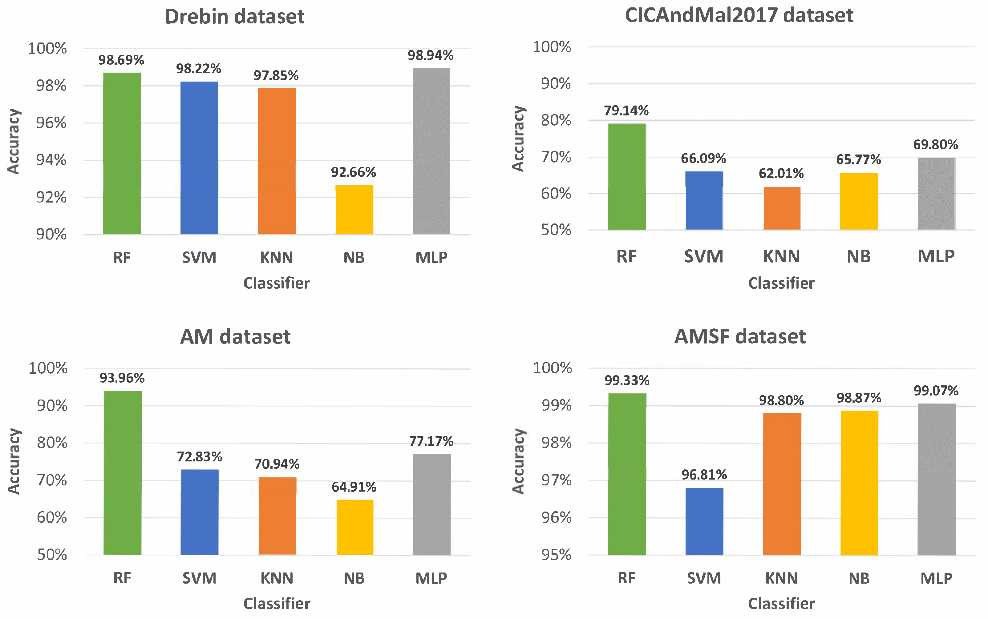
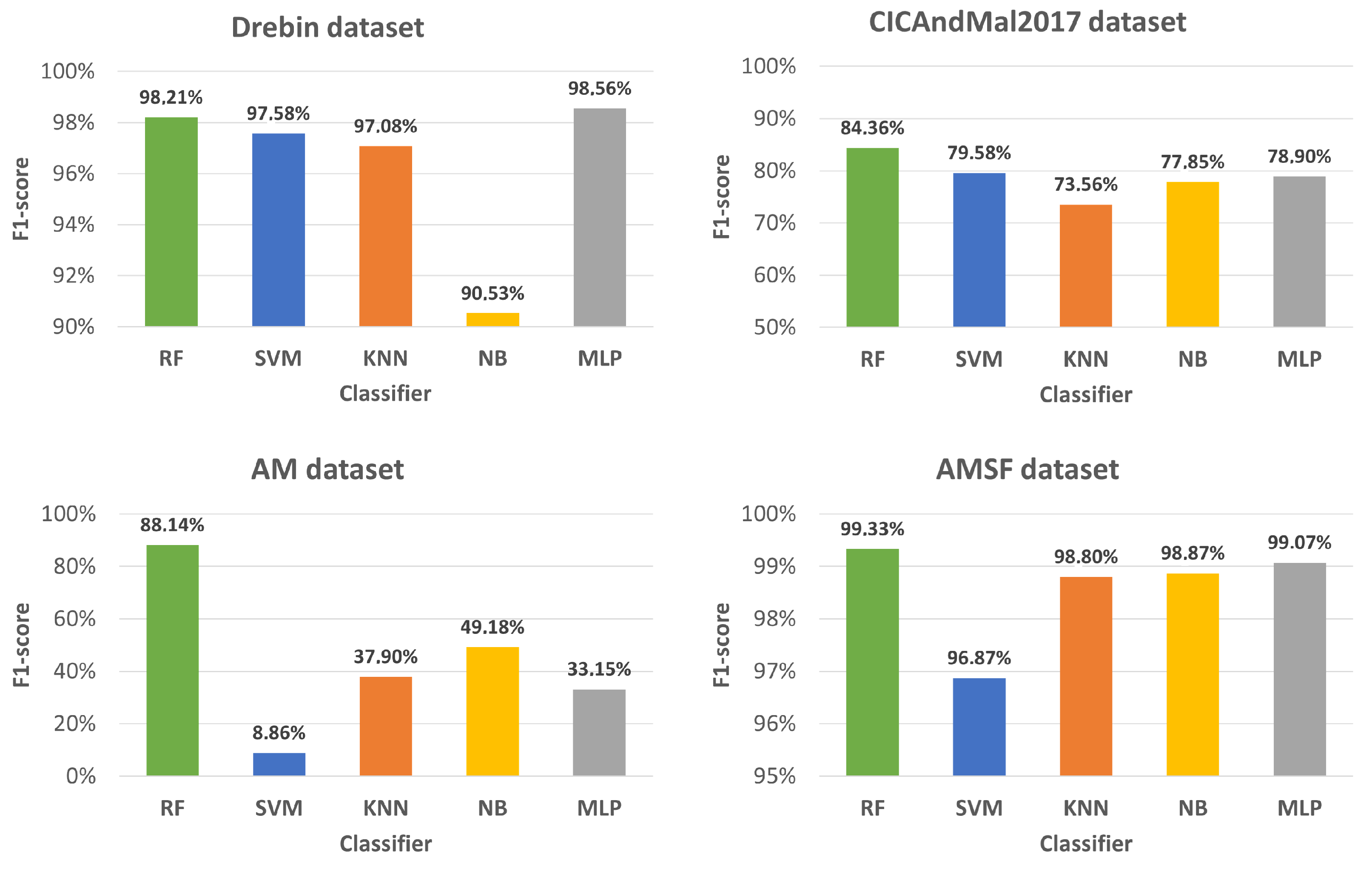
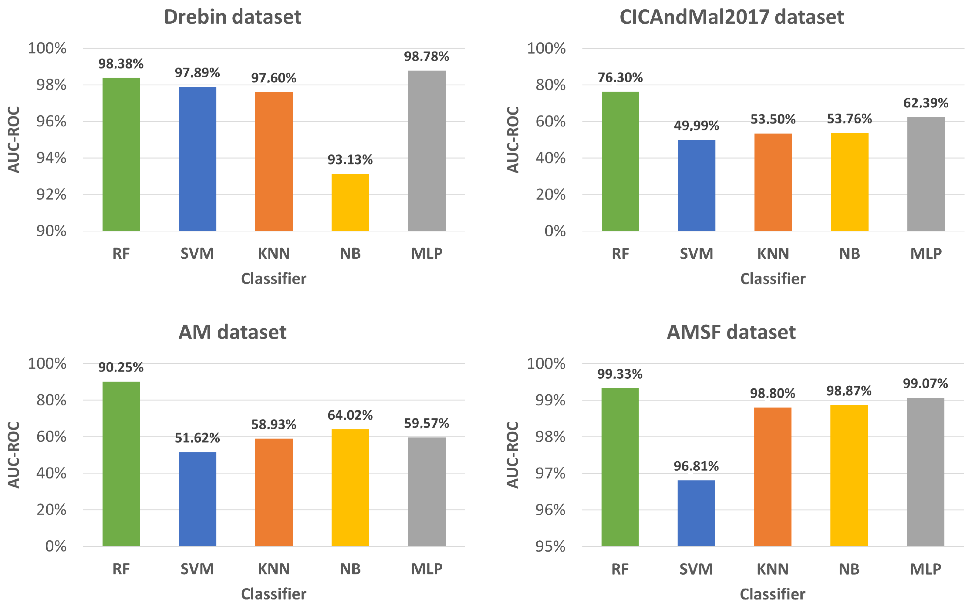
Malware in Android applications affects millions of users worldwide and is constantly evolving. Thus, its detection is a current and relevant problem. In the past few years, ML approaches have been proposed to mitigate malware in mobile applications. In this study, a prototype that resorts to ML techniques to detect malware in Android applications was developed. This task was formulated as a binary classification problem, and public domain datasets (Drebin, CICAndMal2017, AM, and AMSF) were used. Experiments were performed with RF, SVM, KNN, NB, and MLP classifiers, showing that the RF and SVM classifiers are the most suited for this problem.
Data pre-processing techniques were also explored to improve the results. Emphasis was given to FS by applying the RRFS approach to obtain the most relevant and non-redundant subset of features. Although RRFS provided slightly worse results regarding the evaluation metrics, these were arguably compensated for by the dimensionality reduction achieved in each of the used datasets. A reduction of 56% was achieved for the Drebin dataset, 76% for the CICAndMal2017 dataset, 92% for the AM dataset, and 87% for the AMSF dataset. Aside from the dimensionality reduction, RRFS selected the most relevant subset of features to identify the presence of malware. Overall, permissions have a prevalent presence among the most relevant features for Android malware detection.
A nested CV was used to evaluate the trained model better and to tune the ML algorithms hyperparameters, improving the final ML model. As for evaluation metrics, accuracy was used, but, since it can be misleading, other metrics were also applied.
The prototype of the proposed approach was assessed using real-world applications. Overall, the results were negatively impacted by the non-standardization of the dataset’s feature names, which prevented accurate mapping between the extracted features and the most relevant subset of features.
The proposed approach can identify the most decisive features to classify an app as malware and greatly reduce the data dimensionality while achieving good results in identifying malware in Android applications across the various evaluation metrics.
In future work, more up-to-date datasets should be made available and used, and DL approaches and others should be further explored. Furthermore, the proposed approach could be extended to hybrid analysis and/or addressing this problem with a multiclass approach instead of a binary one. Lastly, the feature names across the datasets should have a more uniform designation and be aligned with the names of the features extracted from APK files.

Author Contributions

Conceptualization, A.F.; methodology, A.F.; software, C.P.; validation, C.P., A.F. and M.F.; writing—original draft preparation, C.P.; and writing—review and editing, C.P., A.F. and M.F. All authors have read and agreed to the published version of the manuscript.

Funding

This research was partially funded by FCT—Fundação para a Ciência e a Tecnologia, under grants number SFRH/BD/145472/2019 and UIDB/50008/2020; Instituto de Telecomunicações; and Portuguese Recovery and Resilience Plan, through project C645008882-00000055 (NextGenAI, CenterforResponsibleAI).

Institutional Review Board Statement

Not applicable.

Informed Consent Statement

Not applicable.

Data Availability Statement

The code and data are publicly available at https://github.com/CatarinaPalma-325/Android-Malware-Detection-with-Machine-Learning, accessed on 29 December 2023.

Conflicts of Interest

The authors declare no conflicts of interest.

References

  1. How Many People Have Smartphones?|Oberlo. Available online: https://www.oberlo.com/statistics/how-many-people-have-smartphones (accessed on 29 December 2023).
  2. Turner, A. Android vs. Apple Market Share: Leading Mobile OS. 2023. Available online: https://www.bankmycell.com/blog/android-vs-apple-market-share/ (accessed on 29 December 2023).
  3. How Many Apps in Google Play Store? 2023. Available online: https://www.bankmycell.com/blog/number-of-google-play-store-apps/ (accessed on 29 December 2023).
  4. Alkahtani, H.; Aldhyani, T.H. Artificial intelligence algorithms for malware detection in Android-operated mobile devices. Sensors 2022, 22, 2268. [Google Scholar] [CrossRef] [PubMed]
  5. Pektaş, A.; Çavdar, M.; Acarman, T. Android Malware Classification by Applying Online Machine Learning. In Computer and Information Sciences; Czachórski, T., Gelenbe, E., Grochla, K., Lent, R., Eds.; Springer International Publishing: Cham, Switzerland, 2016; pp. 72–80. [Google Scholar]
  6. Islam, R.; Sayed, M.I.; Saha, S.; Hossain, M.J.; Masud, M.A. Android malware classification using optimum feature selection and ensemble machine learning. Internet Things Cyber-Phys. Syst. 2023, 3, 100–111. [Google Scholar] [CrossRef]
  7. Keyvanpour, M.R.; Barani Shirzad, M.; Heydarian, F. Android malware detection applying feature selection techniques and machine learning. Multimed. Tools Appl. 2023, 82, 9517–9531. [Google Scholar] [CrossRef]
  8. Martín, A.; Calleja, A.; Menéndez, H.D.; Tapiador, J.; Camacho, D. ADROIT: Android malware detection using meta-information. In Proceedings of the 2016 IEEE Symposium Series on Computational Intelligence (SSCI), Athens, Greece, 6–9 December 2016; pp. 1–8. [Google Scholar]
  9. Kouliaridis, V.; Kambourakis, G. A comprehensive survey on machine learning techniques for Android malware detection. Information 2021, 12, 185. [Google Scholar] [CrossRef]
  10. Wu, Q.; Zhu, X.; Liu, B. A survey of Android malware static detection technology based on machine learning. Mob. Inform. Syst. 2021, 2021, 8896013. [Google Scholar] [CrossRef]
  11. Palma, C.; Ferreira, A.; Figueiredo, M. On the use of machine learning techniques to detect malware in mobile applications. In Proceedings of the 14th Simpósio de Informática (INForum), Porto, Portugal, 7–8 September 2023; Available online: https://www.inforum2023.org/Atas/paper_6478/6478-CR.pdf (accessed on 29 December 2023).
  12. Muzaffar, A.; Hassen, H.R.; Lones, M.A.; Zantout, H. An in-depth review of machine learning based Android malware detection. Comput. Secur. 2022, 121, 102833. [Google Scholar] [CrossRef]
  13. Alqahtani, E.J.; Zagrouba, R.; Almuhaideb, A. A Survey on Android Malware Detection Techniques Using Machine Learning Algorithms. In Proceedings of the 2019 Sixth International Conference on Software Defined Systems (SDS), Rome, Italy, 10–13 July 2019; pp. 110–117. [Google Scholar]
  14. Android Malware Dataset for Machine Learning|Kaggle. Available online: https://www.kaggle.com/datasets/shashwatwork/android-malware-dataset-for-machine-learning (accessed on 29 December 2023).
  15. Android Permission Dataset|Kaggle. Available online: https://www.kaggle.com/datasets/saurabhshahane/android-permission-dataset (accessed on 29 December 2023).
  16. Android Malware Dataset|Kaggle. Available online: https://www.kaggle.com/datasets/saurabhshahane/android-malware-dataset (accessed on 29 December 2023).
  17. Android Malware Static Feature Dataset (6 Datasets)|Kaggle. Available online: https://www.kaggle.com/datasets/laxman1216/android-static-features-datasets6-features (accessed on 29 December 2023).
  18. Data Preprocessing in Machine Learning [Steps & Techniques]. Available online: https://www.v7labs.com/blog/data-preprocessing-guide (accessed on 29 December 2023).
  19. Ferreira, A.; Figueiredo, M. Efficient feature selection filters for high-dimensional data. Pattern Recognit. Lett. 2012, 33, 1794–1804. [Google Scholar] [CrossRef]
  20. Chawla, N.V.; Bowyer, K.W.; Hall, L.O.; Kegelmeyer, W.P. SMOTE: Synthetic minority over-sampling technique. J. Artif. Intell. Res. 2002, 16, 321–357. [Google Scholar] [CrossRef]
  21. Witten, I.; Frank, E.; Hall, M.; Pal, C. Data Mining: Practical Machine Learning Tools and Techniques, 4th ed.; Morgan Kauffmann: Burlington, MA, USA, 2016. [Google Scholar]
  22. Breiman, L. Random forests. Mach. Learn. 2001, 45, 5–32. [Google Scholar] [CrossRef]
  23. Rokach, L.; Maimon, O. Top-down induction of decision trees classifiers—A survey. IEEE Trans. Syst. Man Cybern. Part C Appl. Rev. 2005, 35, 476–487. [Google Scholar] [CrossRef]
  24. Alpaydin, E. Introduction to Machine Learning, 2nd ed.; The MIT Press: Cambridge, MA, USA, 2010. [Google Scholar]
  25. Vapnik, V. The Nature of Statistical Learning Theory; Springer: Berlin/Heidelberg, Germany, 1999. [Google Scholar]
  26. Support Vector Machines (SVM)—An Overview|By Rushikesh Pupale|Towards Data Science. Available online: https://towardsdatascience.com/https-medium-com-pupalerushikesh-svm-f4b42800e989 (accessed on 29 December 2023).
  27. Aha, D.; Kibler, D.; Albert, M. Instance-based learning algorithms. Mach. Learn. 1991, 6, 37–66. [Google Scholar] [CrossRef]
  28. Duda, R.; Hart, P.; Stork, D. Pattern Classification, 2nd ed.; John Wiley & Sons: Hoboken, NJ, USA, 2001. [Google Scholar]
  29. Haykin, S. Neural Networks: A Comprehensive Foundation, 2nd ed.; Prentice Hall: Upper Saddle River, NJ, USA, 1999. [Google Scholar]
  30. Bishop, C. Neural Networks for Pattern Recognition; Oxford University Press: Oxford, UK, 1995. [Google Scholar]
  31. AlOmari, H.; Yaseen, Q.M.; Al-Betar, M.A. A Comparative Analysis of Machine Learning Algorithms for Android Malware Detection. Procedia Comput. Sci. 2023, 220, 763–768. [Google Scholar] [CrossRef]
  32. Kouliaridis, V.; Kambourakis, G.; Peng, T. Feature Importance in Android Malware Detection. In Proceedings of the 2020 IEEE 19th International Conference on Trust, Security and Privacy in Computing and Communications (TrustCom), Guangzhou, China, 29 December 2020–1 January 2021; pp. 1449–1454. [Google Scholar] [CrossRef]
  33. Kouliaridis, V.; Potha, N.; Kambourakis, G. Improving Android Malware Detection through Dimensionality Reduction Techniques. In Machine Learning for Networking; Renault, É., Boumerdassi, S., Mühlethaler, P., Eds.; Springer International Publishing: Cham, Switzerland, 2021; pp. 57–72. [Google Scholar]
  34. Kouliaridis, V.; Kambourakis, G.; Geneiatakis, D.; Potha, N. Two Anatomists Are Better than One—Dual-Level Android Malware Detection. Symmetry 2020, 12, 1128. [Google Scholar] [CrossRef]
  35. Potha, N.; Kouliaridis, V.; Kambourakis, G. An extrinsic random-based ensemble approach for android malware detection. Connect. Sci. 2021, 33, 1077–1093. [Google Scholar] [CrossRef]
  36. Alqahtani, A.; Azzony, S.; Alsharafi, L.; Alaseri, M. Web-Based Malware Detection System Using Convolutional Neural Network. Digital 2023, 3, 273–285. [Google Scholar] [CrossRef]
  37. Zhang, S.; Hu, C.; Wang, L.; Mihaljevic, M.J.; Xu, S.; Lan, T. A Malware Detection Approach Based on Deep Learning and Memory Forensics. Symmetry 2023, 15, 758. [Google Scholar] [CrossRef]
  38. Alomari, E.S.; Nuiaa, R.R.; Alyasseri, Z.A.A.; Mohammed, H.J.; Sani, N.S.; Esa, M.I.; Musawi, B.A. Malware Detection Using Deep Learning and Correlation-Based Feature Selection. Symmetry 2023, 15, 123. [Google Scholar] [CrossRef]
  39. Akhtar, M.S.; Feng, T. Malware Analysis and Detection Using Machine Learning Algorithms. Symmetry 2022, 14, 2304. [Google Scholar] [CrossRef]
  40. Hashmi, S.A. Malware Detection and Classification on Different Dataset by Hybridization of CNN and Machine Learning. Int. J. Intell. Syst. Appl. Eng. 2023, 12, 650–667. [Google Scholar]
  41. Djenna, A.; Bouridane, A.; Rubab, S.; Marou, I.M. Artificial Intelligence-Based Malware Detection, Analysis, and Mitigation. Symmetry 2023, 15, 677. [Google Scholar] [CrossRef]
  42. Yang, S.; Wang, Y.; Xu, H.; Xu, F.; Chen, M. An Android Malware Detection and Classification Approach Based on Contrastive Lerning. Comput. Secur. 2022, 123, 102915. [Google Scholar] [CrossRef]
  43. Lu, K.; Cheng, J.; Yan, A. Malware Detection Based on the Feature Selection of a Correlation Information Decision Matrix. Mathematics 2023, 11, 961. [Google Scholar] [CrossRef]
  44. Adebayo, O.S.; Abdul Aziz, N. Improved malware detection model with apriori association rule and particle swarm optimization. Secur. Commun. Netw. 2019, 2019, 2850932. [Google Scholar] [CrossRef]
  45. Zhang, Y.; Yang, S.; Xu, L.; Li, X.; Zhao, D. A Malware Detection Framework Based on Semantic Information of Behavioral Features. Appl. Sci. 2023, 13, 12528. [Google Scholar] [CrossRef]
  46. Daoudi, N.; Samhi, J.; Kabore, A.K.; Allix, K.; Bissyandé, T.F.; Klein, J. DexRay: A Simple, yet Effective Deep Learning Approach to Android Malware Detection Based on Image Representation of Bytecode. In Deployable Machine Learning for Security Defense; Wang, G., Ciptadi, A., Ahmadzadeh, A., Eds.; Springer International Publishing: Cham, Switzerland, 2021; pp. 81–106. [Google Scholar]
  47. KabakuŞ, A.T. Hybroid: A Novel Hybrid Android Malware Detection Framework. Erzincan Univ. J. Sci. Technol. 2021, 14, 331–356. [Google Scholar] [CrossRef]
  48. Aboaoja, F.A.; Zainal, A.; Ghaleb, F.A.; Al-rimy, B.A.S.; Eisa, T.A.E.; Elnour, A.A.H. Malware Detection Issues, Challenges, and Future Directions: A Survey. Appl. Sci. 2022, 12, 8482. [Google Scholar] [CrossRef]
  49. Agrawal, P.; Trivedi, B. A Survey on Android Malware and their Detection Techniques. In Proceedings of the 2019 IEEE International Conference on Electrical, Computer and Communication Technologies (ICECCT), Coimbatore, India, 20–22 February 2019; pp. 1–6. [Google Scholar] [CrossRef]
  50. Almomani, I.; Ahmed, M.; El-Shafai, W. Android malware analysis in a nutshell. PLoS ONE 2022, 17, e0270647. [Google Scholar] [CrossRef]
  51. Deldar, F.; Abadi, M. Deep Learning for Zero-Day Malware Detection and Classification: A Survey. ACM Comput. Surv. 2023, 56, 1–37. [Google Scholar] [CrossRef]
  52. Faruki, P.; Bhan, R.; Jain, V.; Bhatia, S.; El Madhoun, N.; Pamula, R. A Survey and Evaluation of Android-Based Malware Evasion Techniques and Detection Frameworks. Information 2023, 14, 374. [Google Scholar] [CrossRef]
  53. Gyamfi, N.K.; Goranin, N.; Ceponis, D.; Čenys, H.A. Automated System-Level Malware Detection Using Machine Learning: A Comprehensive Review. Appl. Sci. 2023, 13, 11908. [Google Scholar] [CrossRef]
  54. Liu, K.; Xu, S.; Xu, G.; Zhang, M.; Sun, D.; Liu, H. A Review of Android Malware Detection Approaches Based on Machine Learning. IEEE Access 2020, 8, 124579–124607. [Google Scholar] [CrossRef]
  55. Meijin, L.; Zhiyang, F.; Junfeng, W.; Luyu, C.; Qi, Z.; Tao, Y.; Yinwei, W.; Jiaxuan, G. A Systematic Overview of Android Malware Detection. Appl. Artif. Intell. 2022, 36, 2007327. [Google Scholar] [CrossRef]
  56. Naseer, M.; Rusdi, J.F.; Shanono, N.M.; Salam, S.; Muslim, Z.B.; Abu, N.A.; Abadi, I. Malware Detection: Issues and Challenges. J. Phys. Conf. Ser. 2021, 1807, 012011. [Google Scholar] [CrossRef]
  57. Odusami, M.; Abayomi-Alli, O.; Misra, S.; Shobayo, O.; Damasevicius, R.; Maskeliunas, R. Android Malware Detection: A Survey. In Applied Informatics; Florez, H., Diaz, C., Chavarriaga, J., Eds.; Springer International Publishing: Cham, Switzerland, 2018; pp. 255–266. [Google Scholar]
  58. Razgallah, A.; Khoury, R.; Hallé, S.; Khanmohammadi, K. A survey of malware detection in Android apps: Recommendations and perspectives for future research. Comput. Sci. Rev. 2021, 39, 100358. [Google Scholar] [CrossRef]
  59. Souri, A.; Hosseini, R. A State-of-the-Art Survey of Malware Detection Approaches Using Data Mining Techniques. Hum.-Centric Comput. Inf. Sci. 2018, 8, 3. [Google Scholar] [CrossRef]
  60. Qiu, J.; Zhang, J.; Luo, W.; Pan, L.; Nepal, S.; Xiang, Y. A Survey of Android Malware Detection with Deep Neural Models. ACM Comput. Surv. 2020, 53, 1–36. [Google Scholar] [CrossRef]
  61. Vasani, V.; Bairwa, A.K.; Joshi, S.; Pljonkin, A.; Kaur, M.; Amoon, M. Comprehensive Analysis of Advanced Techniques and Vital Tools for Detecting Malware Intrusion. Electronics 2023, 12, 4299. [Google Scholar] [CrossRef]
  62. Wang, D.; Chen, T.; Zhang, Z.; Zhang, N. A Survey of Android Malware Detection Based on Deep Learning. In Machine Learning for Cyber Security; Xu, Y., Yan, H., Teng, H., Cai, J., Li, J., Eds.; Springer International Publishing: Cham, Switzerland, 2023; pp. 228–242. [Google Scholar]
  63. Guyon, I.; Gunn, S.; Nikravesh, M.; Zadeh, L. (Eds.) Feature Extraction, Foundations and Applications; Springer: Berlin/Heidelberg, Germany, 2006. [Google Scholar]
  64. Guyon, I.; Elisseeff, A. An introduction to variable and feature selection. J. Mach. Learn. Res. (JMLR) 2003, 3, 1157–1182. [Google Scholar]
  65. sklearn.model_selection.GridSearchCV—Scikit-Learn 1.3.1 Documentation. Available online: https://scikit-learn.org/stable/modules/generated/sklearn.model_selection.GridSearchCV.html (accessed on 29 December 2023).
  66. Not So Boring Android Malware|Android-Malware-Samples. Available online: https://maldroid.github.io/android-malware-samples/ (accessed on 29 December 2023).
Figure 1. Components of an Android application (app).
Information 15 00025 g001
Figure 2. Partial block diagram of the proposed approach: the data pre-processing stage, which is composed of handling missing values, numerosity balancing, and feature selection. The vertical arrow points to the continuation of the ML pipeline, and the right-hand side arrow highlights that our approach identifies the most relevant features for the feature extraction module.
Information 15 00025 g002
Figure 3. Partial block diagram of the proposed approach: data splitting for training and testing of the model with standard evaluation metrics. We also provide a validation set to perform hyperparameter tuning. The right-hand side arrow with input data refers to the use of data from real-world applications.
Information 15 00025 g003
Figure 4. Full block diagram of the ML module, aggregating all the stages referenced in Figure 2 and Figure 3 as well as the hyperparameter tunning stage.
Information 15 00025 g004
Figure 5. Full block diagram of the proposed approach with the ML module and the Android applications and feature extraction modules.
Information 15 00025 g005
Figure 6. Developed Android applications: ‘App1’ (two images on the left hand-side), ‘App2’, and ‘App3’.
Information 15 00025 g006
Figure 7. Accuracy (%) obtained with each classifier (RF, SVM, KNN, NB, and MLP) for each dataset. The average accuracy per classifier is 92.78%, 83.48%, 82.40%, 80.55%, and 86.24%, respectively.
Information 15 00025 g007
Figure 8. F1-score (%) obtained with each classifier (RF, SVM, KNN, NB, and MLP) for each dataset. The average F1-score per classifier is 92.51%, 70.72%, 76.83%, 79.10%, and 77.42%, respectively.
Information 15 00025 g008
Figure 9. AUC-ROC (%) obtained with each classifier (RF, SVM, KNN, NB, and MLP) for each dataset. The average AUC-ROC per classifier is 91.06%, 74.07%, 77.20%, 77.44%, and 79.95%, respectively.
Information 15 00025 g009
Figure 10. Accuracy (%) obtained, with the RF and SVM classifiers, for the AM dataset after applying different methods to deal with missing values.
Information 15 00025 g010
Figure 11. Number of features for each dataset, by not applying RRFS (original baseline) nnd by applying it with MM and FR relevance metrics.
Information 15 00025 g011
Table 1. Summary of some results reported in existing approaches.
StudyDatasetClassifierAcc (%)
Alkahtani and Aldhyani [4]DrebinSVM80.71
KNN81.57
CICAndMal2017SVM100.0
KNN90.00
Keyvanpour et al. [7]DrebinRF (with 100 DT)99.49
Islam et al. [6]CCCS-CIC-AndMal2020Ensemble95.00
AlOmari et al. [31]CICMalDroid2020LightGBM95.49
Table 2. Summary of the datasets considered in the experimental evaluation.
DatasetInstances (n)Features (d)Available in
Drebin15,036215[14]
CICAndMal201729,999110[15]
AM11,476182[16]
AMSF5019966[17]
Table 3. Class distribution for each dataset.
DatasetBenign, nMalicious, nTotal, n
Drebin9476 (63.02%)5560 (36.98%)15,036
CICAndMal20179999 (33.33%)20,000 (66.67%)29,999
AM8058 (70.22%)3418 (29.78%)11,476
AMSF2508 (49.97%)2511 (50.03%)5019
Table 4. Categorical and non-categorical features (d) in each dataset.
DatasetCategorical dNon-Categorical dTotal d
Drebin1214215
CICAndMal20175105110
AM12170182
AMSF0966966
Table 5. Number of missing values in each dataset.
DatasetNumber of Missing Values
Drebin0
CICAndMal2017204
AM19,888
AMSF0
Table 6. Accuracy (Acc), F 1 score and AUC-ROC with min–max normalization, using the RF and SVM classifiers on the CICAndMal2017 and AM datasets.
ClassifierDatasetNormalizationAcc (%) F 1 Score (%)AUC-ROC (%)
RFCICAndMal2017None79.8184.8277.40
Min–max79.6284.7277.06
RFAMNone93.2888.0290.28
Min–max93.2888.0590.33
SVMCICAndMal2017None66.1378.9651.51
Min–max70.8179.7163.22
SVMAMNone70.230.0050.00
Min–max90.8882.7785.89
Table 7. Accuracy (Acc) and Recall (Rec) values for the RF and SVM classifiers with the different numerosity balancing approaches for the AM dataset.
ClassifierNumerosity BalancingAcc (%)Rec (%)
RFNone93.2883.02
Random undersampling91.3686.44
Random oversampling96.2896.07
SMOTE94.0691.39
SVMNone70.8186.00
Random undersampling89.1882.44
Random oversampling89.4782.75
SMOTE88.8181.42
Table 8. Accuracy (Acc) obtained with the SVM classifier for each dataset, by not applying RRFS (original baseline) and by applying it with MM and FR relevance metrics.
DatasetRRFSAcc (%)
DrebinNone98.50
MM94.71
FR96.66
CICAndMal2017None71.69
MM60.04
FR68.52
AMNone89.47
MM86.99
FR84.55
AMSFNone99.53
MM99.87
FR98.41
Table 9. Comparison of the experimental results, in terms of Accuracy (%), obtained by Alkahtani and Aldhyani [4] with the SVM classifier with the ones obtained with the proposed approach using the same classifier.
DatasetAlkahtani and AldhyaniProposed
Drebin80.7197.47
CICAndMal2017100.0073.22
Disclaimer/Publisher’s Note: The statements, opinions and data contained in all publications are solely those of the individual author(s) and contributor(s) and not of MDPI and/or the editor(s). MDPI and/or the editor(s) disclaim responsibility for any injury to people or property resulting from any ideas, methods, instructions or products referred to in the content.

