1. Introduction to Information Graph Theory
Real-world networking systems comprising functional units that interact with each other at different and disparate temporal and spatial scales are often metaphorically represented by finite connected undirected graphs [
1]. In graph models, the vertices embody the system functional units, and the edges sketch the various interactions between these units. Graph models are useful for computer networking, sociology, urban morphology, smart city networks, chemistry, engineering, communication, logistics and management, security applications, etc., as they help us to answer the fundamental question about relations between the
local and
global properties of a networking system.
In our work, we assess the quality of these relations by using some information quantities at different graph connectivity scales, ranging from the connectivity between the nearest neighbors to the connectivity with respect to infinitely long paths available in the graph. The proposed information approach to the description of graph structures (which can be called information graph theory) may be especially useful for the assessment of communication efficiency between individual systems’ units at different time and connectivity scales.
One possible application of graph information theory is the design of network-on-chip (NoC), or network-based communications subsystems on an integrated circuit, most typically between semiconductor intellectual property cores schematizing various functions of the computer system in a system on a single chip [
2]. (We profoundly thank our reviewer for pointing us at the possible NoC-related application of graph information theory.) NoCs provide the advantage of customized architecture, increased scalability, and bandwidth and come in many network topologies, many of which are still experimental [
3].
The interconnections between multiple cores on a chip present a considerable influence on the performance and communication of the chip design regarding the throughput, end-to-end delay, and packet loss ratio. Based on the huge amount of supported heterogeneous cores, efficient communication between the associated processors has to be considered at all levels of system design to ensure global interconnection [
4]. Although hierarchical architectures have addressed the majority of the associated challenges of the traditional interconnection techniques, the main limiting factor is scalability, and NoC has proven to be a promising solution. As communicating nodes require a routing algorithm for successful transmission of packets, it is important to design an NoC routing algorithm capable of providing less congested paths, better energy efficiency, and high scalability [
5]. It is important to mention that the same choices of routing algorithms, when considered for more than one performance parameter of the network, do not yield expected results, since different applications exhibit different network performances for the same routing technique [
6]. Fault-tolerant mapping and routing techniques at different levels of an NoC were surveyed in [
7]. In [
8], a method for choosing hierarchical coordinates and a greedy forwarding algorithm for path-finding were presented. Nevertheless, reliability is becoming a major concern in NoC design [
7]. In particular, the accurate predictions of network packet latency, contention delay, and the static and dynamic energy consumption of the network are in demand [
9].
Another evident application field of graph information theory is the study of urban morphology, i.e., urban forms and structures affecting sustainability and urban growth. Along with the spreading of new technologies and the availability of big data, cities are increasingly viewed not simply as places in space but as systems of networks and flows [
10]. This became particularly evident in the concept of a
smart city, as the synergy of architecture, technology, and the
Internet of Things which enables the collection and data exchange of objects embedded with electronics, software, sensors, and network connectivity [
11].
All above-mentioned research problems involve a variety of information quantities resolving uncertainty about evolution of some diffusion processes at different connectivity scales in a graph, and therefore the entire approach to graphs summarized in the present paper may be called information graph theory.
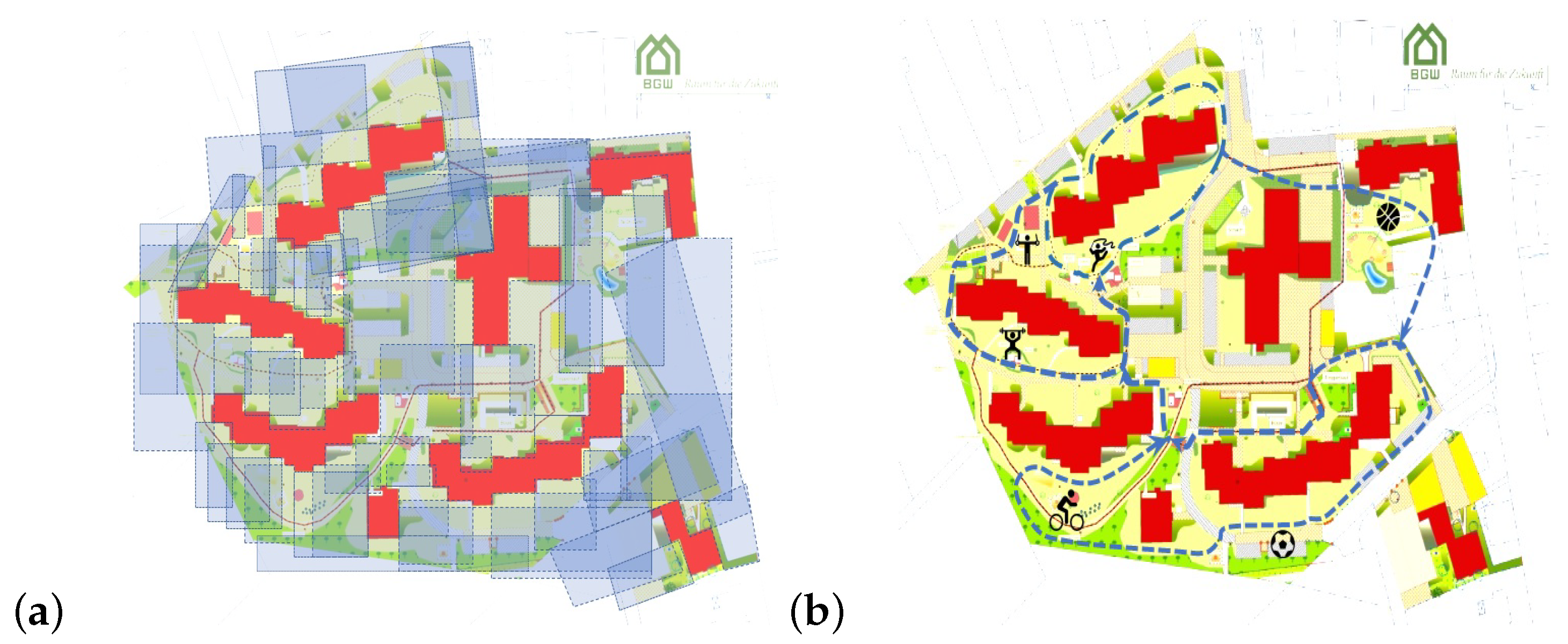
Thinking about transportation in networks—imagine the weekend pedestrian flow in a city downtown area—we may notice that some streets are more preferred by walkers than others. While some urban quarters are visited quite often, others seem to be excluded from the rest of urban fabric, as though being barricaded by invisible gates, literally turning the deserted city block into a ghetto. A widespread belief in the influence of the spatial organization of the built environment on the way people move through urban spaces and meet others by chance was common in architectural and urban thinking for centuries [
12,
13,
14]. The dynamics of poverty areas in London studied over the past century in [
15] has shown that the creation of poverty areas is ultimately a spatial process relating to spatial segregation and poverty. In order to quantify isolation by identifying
the most and least probable paths through the areas with respect to a certain exploration strategy, in the present paper we put forward a concept of
walkability.
Navigation focuses on locating a walker’s position with respect to known locations, traversed paths, and structural patterns in the environment [
16]. In the probabilistic setting,
navigability would represent
a share of predictable information about the future location of a traveler given their walking history and the present location. The predictable information about the future location of a walker is obtained with the use of two major navigation strategies, known as
path integration (which allows for keeping track of the position and heading while exploring a new space) and
landmark-based piloting (re-calculating position of a traveler while in a familiar environment), working in concert during navigation in humans and animals [
16].
Finally, as such a circumstance appears quite often in the context of science and technology, we may pose the following question: How long should one observe a networking system for the information collected to be enough to draw a reliable conclusion about its evolution in the long run? Of course, an answer to the above-posed question ultimately depends on the structural complexity of a system (that can often be represented by a graph), the dynamics of the processes in question, as well as on the chosen graph exploration strategy—all are difficult to quantify, in general. In the present paper, we call such a deep, penetrating discernment of the system’s nature and evolution perspicacity and discuss and quantify it in the framework of a proposed model.
In our work, we put forward a toy model, in which the questions of interest may receive quantitative answers. The role of a complex system will be played by a finite connected undirected graph providing a scene for
isotropic and a variety of
anisotropic diffusions, i.e., different types of
random walks, forming the
canonical statistical ensembles of walks defined in graphs (see
Section 3). Uncertainty about the current state in Markov chains contains
predictable (apparent uncertainty) and
unpredictable (true uncertainty) information components: the conditional mutual information quantities among the past, present, and future states of the chain (see
Section 2). The amount of predictable information can be viewed as a divergence between the
ensemble average (defined with respect to the stationary distribution of random walks) and the
time-average of walks describing the probability of observing a walker in a unit time of random walks. Consequently, the amount of uncertainty about the future location of random walkers in the graph that can be resolved by using the standard navigation strategies, such as
path integration (based on the entire history of travels) and
landmark-based piloting (based on the present location of the walker), can be viewed as a
navigability potential of a node in the given graph structure with respect to the chosen exploration strategy (the type of diffusion process) (see
Section 4). We call the opposite potential characterizing the amount of true uncertainty about the walker’s location in the graph
strive, which is quantified as the expected exploration time of a node’s neighborhood by the given type of random walk (
Section 4). Information flows associated with the diffusion processes in graphs (see
Section 3 and
Section 5) can be viewed as the stochastic point processes, called
determinantal process or fermionic processes [
17], because the corresponding densities are the squared wedge-products (determinants) of eigenvectors of the symmetrized transition matrices. We use the properties of the determinantal processes to assess
perspicacity and
walkability in graphs (see
Section 3 and
Section 5). The perfect perspicacity is possible only for the processes that enjoy the same type of symmetry. In
Section 6, we discuss an example of the walkability analysis in urban neighborhoods and, eventually, conclude on a discussion of graph information theory and its applications in the last section.
2. Predictable and Unpredictable Information in Markov Chains
The resolution of uncertainty about future events is known as information [
18]. For example, each coin flip reveals a single bit of information. The side repeating probability
in the coin tossing sequence does not affect the amount of information released at every flip, but rather determines a
share of predictable and unpredictable information components in every released bit of information [
19,
20,
21,
22]. Indeed, the forthcoming state of the Markov chain describing tossing of a biased coin is completely predictable for
when coin tossing generates the stationary sequences
heads, heads, heads,… or
tails, tails, tails, …, as well as for
when an alternating sequence of states arises. However, the side of the coin that will come up on the next toss is utterly unpredictable if
.
For a Markov chain
,
defined over a finite set of
N states by a (stationary) irreducible, row-stochastic transition probability matrix
, the expected amount of uncertainty about a state over infinitely long sequences is given by the Boltzmann–Gibbs–Shannon entropy [
20,
22,
23,
24],
where
is a stationary distribution of states over the chain, i.e., the left eigenvector of the Markov chain transition matrix,
belonging to the major eigenvalue 1. In all information-related calculations, we shall assume that
As the information shared between the past and future in Markov chains is transmitted only through the present, the time average of the conditional entropy of the present state conditioned on all past states simplifies to the entropy rate [
19,
22,
25,
26], viz.,
Then, the following formal decomposition involving one-step conditional entropies [
19,
20,
21,
22],
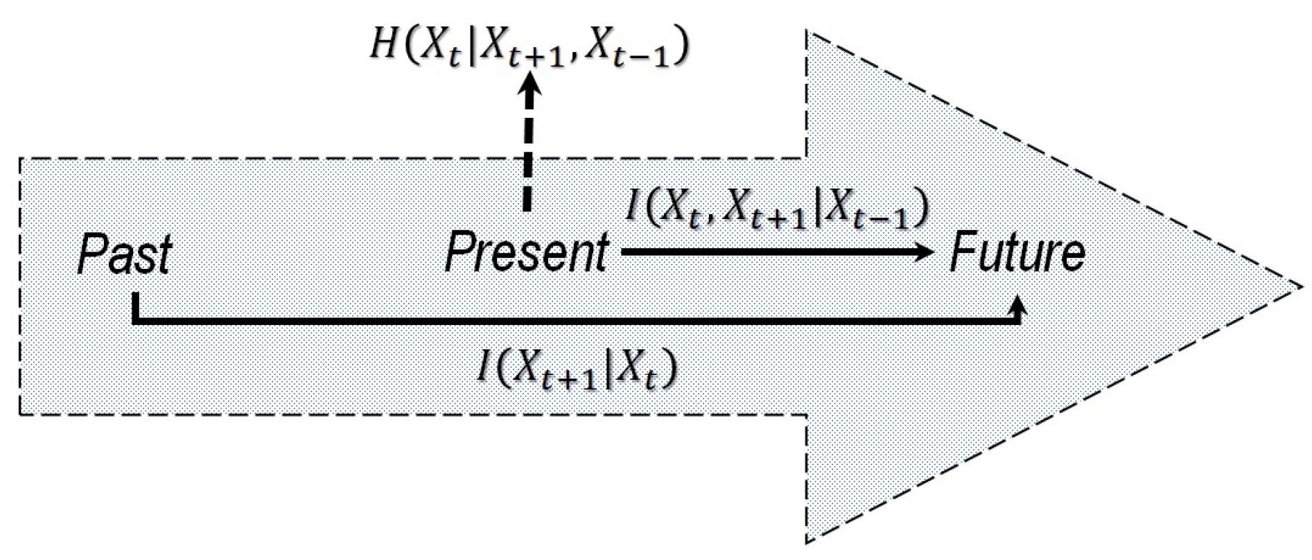
represents the state’s uncertainty as a sum of the following three information components: (i)
, expressing the amount of information about the future state that can be inferred from the entire past history of the chain, excepting for its present state; (ii)
, the mutual information between the future and present states of the chain, expressing the amount of information about the future state that can be inferred from the present state, independently of the past; and (iii)
, expressing the
true uncertainty about the present state of the chain that cannot be resolved by observing the past history and that does not have repercussions for the future evolution of the chain. Assuming that all past states and the present state of the chain are known, we conclude that the first two quantities contribute to the predictable information component of the chain, viz.,
while the last term quantifies the ephemeral, unpredictable information component, viz.,
which exists at the present moment only and then disappears without consequences [
19,
20].
The information diagram for a Markov chain is shown in
Figure 1. In the context of Markov chains, we may interpret or explain a future event either as a consequence of history, or as an immediate outcome of the present event. However, for
, some amount of uncertainty remains unresolved before the event occurs, and such a surprise cannot be avoided, eliminated, or controlled. Given the Markov chain transition matrix
T, the entropy excess
[
19,
20,
21,
22,
27,
28,
29] reads as follows:
The conditional mutual information
between the present and the future states of the chain conditioned on the past state takes the following form [
19,
20,
21,
22]:
The conditional mutual information (
7) quantifies a consequence of the present state for the future evolution of the Markov chain. Finally, the amount of true uncertainty existing only at the present moment of time is the entropy residue [
19,
20,
21,
22], viz.,
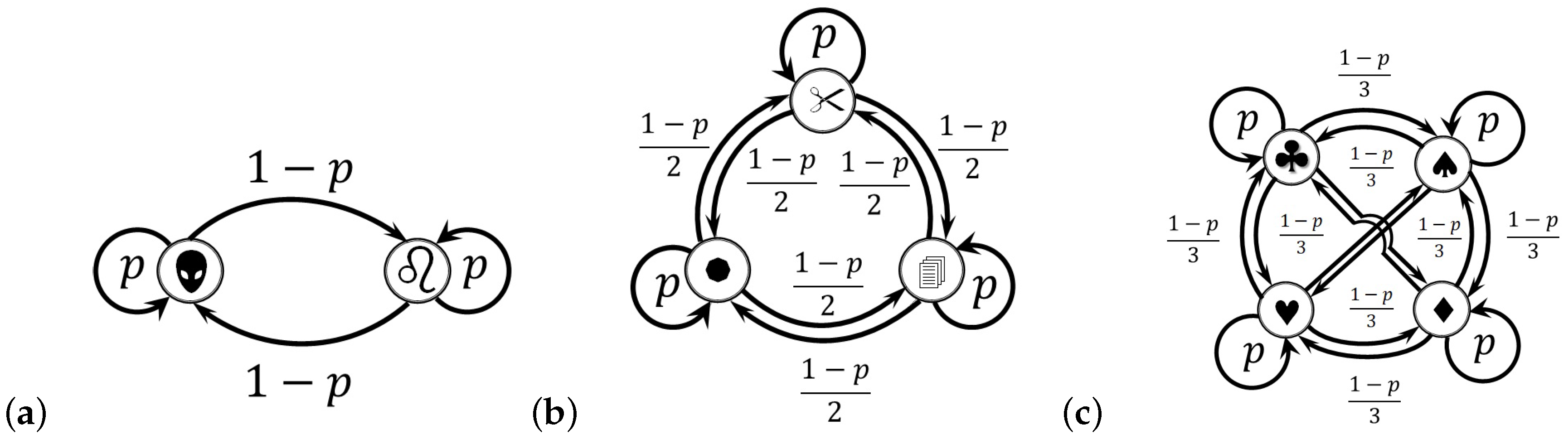
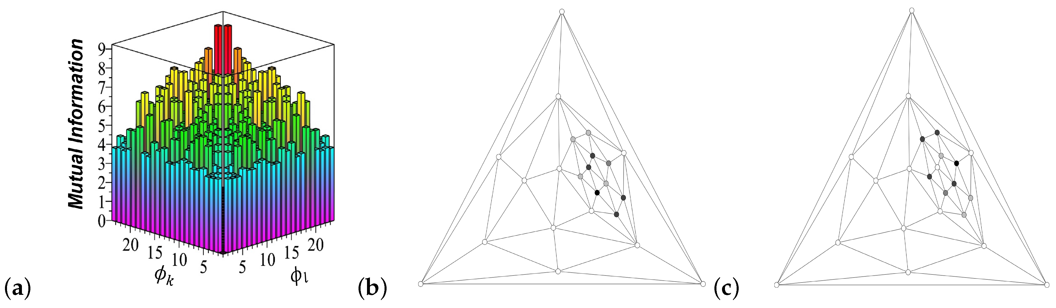
For example, let us consider three games of chance shown in
Figure 2a–c having
and 4 states, respectively. The probability of repeating a state in each game is taken as
. Other transitions are chosen to be equiprobable. For entropy calculations in this section, we use the
N-based logarithm
, so that the information and entropy quantities for these games of chance are measured in
bits,
trits, and
quadrits, respectively. Namely, a single
bit of information is released at every coin flip (see
Figure 2a); one
trit of information is produced at every round of the rock–paper–scissors game (see
Figure 2b); and one
quadrit of information is brought about at every round of the card suit game of four states (see
Figure 2c). The use of different information units allows for comparing the structure of information components for all three games in a single frame (as shown in
Figure 3). Otherwise, the graphs would scale up by
and
if we used bits as a major information unit. The detailed information analysis of a two-state Markov chain shown in
Figure 2a has been developed by us in [
20], and in [
30] we discussed information components in a three-state chain (
Figure 2b). The four-state chain shown in
Figure 2c has never before been discussed.
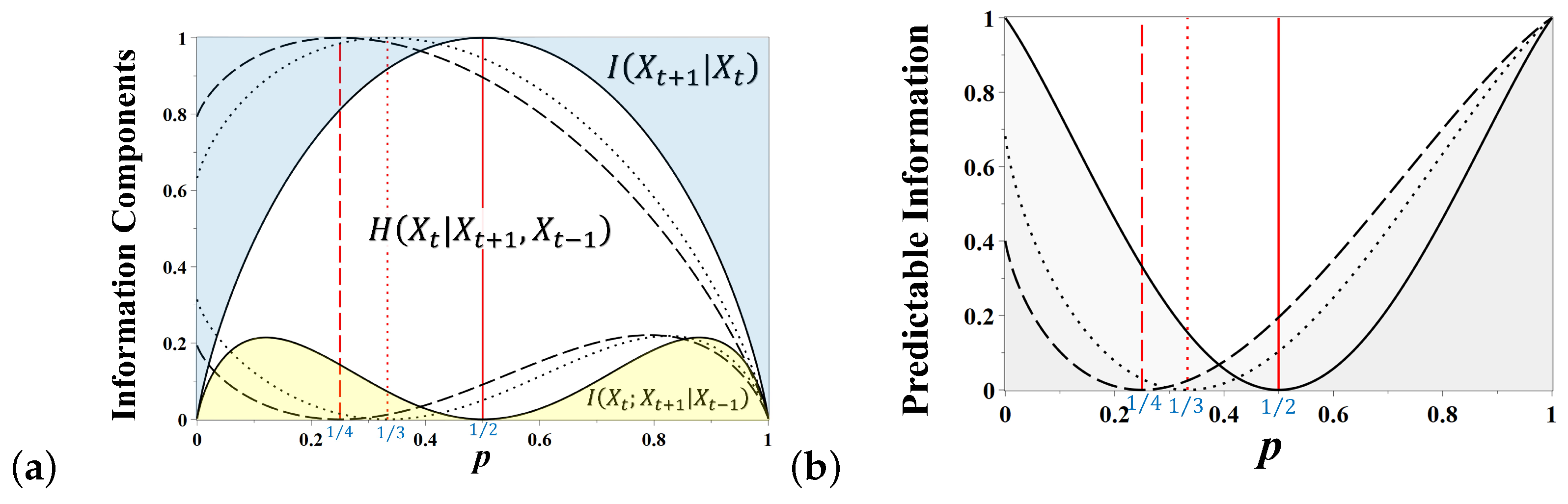
The information components (
6–
8) for all three games shown in
Figure 2 are presented in
Figure 3 as functions of the state repetition probability
p. In
Figure 3a, the predictable information components in a coin tossing game (see
Figure 2a) are indicated by the solid line, and the graph regions representing the predictable information components
and
are highlighted in blue and yellow, respectively.
The future outcome of coin tossing is reliably predictable for
or
when the game generates the stationary alternating or constant sequences of states, respectively. In this case, the entire uncertainty of a state equals the entropy excess (blue in
Figure 3a), viz., 1 bit
As
or
, the reliability of predictions based on the past history of the chain decays; however, the future outcome may then be guessed from the present state of the coin alone, either by alternating the present side of the coin at the next tossing (for
), or by repeating it (for
). The corresponding amount of information,
quantifying the degree of reliability of such a guess, is highlighted by yellow in
Figure 3a. When
, there is a destructive interference between two incompatible hypotheses about the future outcome of coin tossing that causes the gradual attenuation and cancellation of mutual information,
, and the coin becomes fair at
. At this moment, the entire uncertainty of a state equals the amount of true uncertainty quantified by
[
20]. Summing the predictable information components together, we obtain the amount of predictable information about the future outcome of coin tossing as a function of
p, shown in
Figure 3b as a solid line. The coin tossing game (see
Figure 2a) is predictable at
and
, but unpredictable at
when the coin is fair.
The information components for other games of chance (
Figure 2b,c) are presented in
Figure 3a,b by the dotted and dashed lines. The rock–paper–scissors game (
Figure 2b) becomes fair at
, and the relevant information components are shown as dotted lines. The model of a three-sided coin (
susceptible–
infected–
immune) was recently used for assessing pandemic uncertainty on conditions of vaccination and self-isolation [
30]. The card suit game (
Figure 2c) is fair when
, as shown by the dashed lines in
Figure 3a,b. In contrast to the simple coin flipping game, other games of chance, having more possible states, are not completely predictable for
, as they retain a certain degree of uncertainty of symbols in the alternating sequences of chain states.
3. Symmetries and Statistical Ensembles of Walks in Finite Connected Undirected Graphs
A finite connected undirected graph
, in which
V,
, is a set of vertices and
is a set of edges, is defined by a symmetric adjacency matrix,
, such that
, iff
, but
otherwise. The adjacency matrix allows for the following spectral decomposition:
in which
is an orthogonal system of eigenvectors belonging to the ordered real eigenvalues
, where
is simple according to the Perron–-Frobenius theorem [
31].
Graph symmetries: Multiple eigenvalues of the adjacency matrix indicate the presence of non-identity automorphisms in the graph
G [
19,
32,
33,
34,
35,
36]. A group of a graph’s automorphisms
preserving the graph structure is formed by all permutations
defined on the set of graph vertices
V that commute with the graph adjacency matrix,
[
19,
32,
34]. If a non-identical
exists, and
is an eigenvector of the adjacency matrix, such that
then the vector
is another eigenvector of
A belonging to the same eigenvalue
, as
. An automorphism associated with some eigenvalue
of multiplicity
is represented by a low-dimensional
real orthogonal submatrix corresponding to the related block of a permutation matrix. As the eigenvectors of a symmetric adjacency matrix are real and mutually orthogonal,
, it also follows that elements of these eigenvectors are
mapped to each other under the action of
. For example, the major (Perron) eigenvector
of the adjacency matrix of a triangle graph belongs to the maximum eigenvalue
, while another, double eigenvalue
corresponds to the eigenvectors
and
mapped to each other by a simple 2-permutation.
Microcanonical ensemble of walks: The microcanonical ensemble of walks (MCE) is a collection of
n-walks in
G taken with the same probability
for all walks of the same length
n, in which the (Boltzmann constant and) temperature
, and the free energy of
n–walks is defined by the logarithm of the number of
n-walks available in the graph
. For very long walks,
,
, where
, and therefore the intensive free energy (per edge absorbed by a very long MCE walk) equals the graph topological entropy [
21,
22,
37], viz.,
Canonical ensemble of walks: In the canonical ensembles of walks (CNE) defined on
G, each of
walks of length
n available from every node
are taken with equal probability. As
, the CNE walks are defined by the following irreducible row-stochastic transition matrices [
19,
21,
22]:
The CNE walks
are the random walks defining the following stationary distributions (centrality measures [
21,
22]) of nodes:
In particular, the locally isotropic first order random walks, in which a random walker chooses a node to visit with equal probability among all available nearest neighbors,
defines the well-known stationary distribution of nodes (degree centrality), viz.,
[
19,
21,
22]. For
,
, so that the series of transition matrices converges to the Ruelle–Bowen random walk [
38], viz.,
with a stationary distribution
[
39] that is related to the eigenvector centrality of nodes [
40].
Grand canonical ensemble of walks: Finally, the grand canonical ensemble of walks (GCE) describes the statistics of “fluctuations” of the local growth rate of the number of walks available at the node
over a “chemical potential”
of the equiprobable
n-walks in the graph
G, viz.,
In the thermodynamic limit of infinite walks
, the exponential factor representing a node’s “fugacity” takes the following form [
22]:
The limiting distribution of relative fugacity, describing the change of the system of infinitely long walks (free energy of walks) due to adding/removing a node, takes the form of a Fermi—Dirac distribution, viz.,
typical for the distribution of fermions in a single-particle state
i of the energy
The Fermi—Dirac distribution, previously observed only in a quantum system of non-interacting fermions, appears in the model due to the non-interacting quality of walks in the graph, similar to the Pauli exclusion principle allowing for only two possible microstates for each single-particle level [
22].
Determinantal point processes associated with canonical ensembles of walks—Perspicacity: The CNE walks in a connected undirected graph define the determinantal point processes characterized by the probabilities of random currents calculated as the squared determinants of submatrices made up from the elements of eigenvectors of the symmetrized random walk transition matrices. These determinantal point processes provide the properly normalized probability distributions for all nodes, subgraphs, and nodal subsets at all time scales of the corresponding diffusion process [
22]. Slater determinants in quantum mechanics [
41] were historically the first examples of determinantal point processes that later acquired multiple applications in physics, applied mathematics, and statistics [
42,
43,
44,
45]. The symmetrization similarity transformation [
19,
22] makes the Markov matrix
into a symmetric form,
, viz.,
In the rest of this section, we omit the index
in the symmetrized transition matrix (
16) to simplify the notations. The determinantal point processes may be defined for any type of random walk, and the resulting probability distributions indeed vary for different
n. The symmetrized transition matrix (
16) can be written in a spectral form as follows:
, in which
is an orthogonal matrix,
, with columns being the orthonormal eigenvectors
of the symmetrized transition matrix (
16), and
is a diagonal matrix of real valued, ordered eigenvalues of the transition matrix,
. The repeating eigenvalues indicate the presence of symmetries in the diffusion process, and if
is an eigenvector of the symmetrized transition matrix (
16) belonging to the multiple eigenvalue
, then there exists a permutation matrix
, such that
and
is another eigenvector of
belonging to the same eigenvalue
. In the latter case, the symmetry may be represented by a low-dimensional real orthogonal submatrix in
corresponding to the related blocks of a permutation matrix.
As the dynamics of discrete time random walks evolves with powers of the corresponding transition matrix, the eigenvalues for describe the rates of relaxation processes toward a stationary distribution over graph nodes belonging to the maximal eigenvalue . Herewith, the positive eigenvalues , , describe the exponential decay of the relaxation processes (as ), while the negative eigenvalues correspond to damped oscillations, and both fade away within the finite characteristic relaxation times . The characteristic relaxation time of the stationary distribution is taken to be
The
k-th order wedge products,
, are the determinants of the corresponding
k-th order minors of the matrix
. The properties of determinants of submatrices composed of orthonormal vectors were discussed in [
19,
46] in more detail. In particular, the squared determinants of the
k-th order minors of the orthogonal matrix
define the properly normalized probability distributions over the index set
, viz.,
For example, the squared elements of the major eigenvector of the symmetrized transition matrix,
can be considered the squared determinants of the primitive submatrices of size 1, determining the stationary distribution of random walks, viz.,
The corresponding probability
is interpreted as a measure of likeliness to observe a random walker at
in infinite observation time
. Other eigenvectors,
,
, also enjoy the proper normalization,
, and therefore can be interpreted as the ephemeral probability distributions decaying in the finite characteristic time,
.
The squared wedge products,
define the ephemeral probability distributions over pairs of nodes (not necessarily corresponding to graph’s edges) fostered by the modes
and
of the diffusion process, viz.,
,
may be interpreted as the joint probability mass functions (correlation functions) describing the probability amplitudes for a random walker to sojourn at the nodes
i and
j during the characteristic times
and
. Using the properties of determinants, we may expand the probability mass function
into the joint probability of independent observations of the walker at
i and
j during the characteristic times
and
, conditional on obviously incompatible events, such as the simultaneous presence of the random walker at two different nodes, viz.,
If
and
and
are the simple eigenvalues, then the determinants in (
17) equal zero for any
i and
j. Otherwise, if
and
belong to the same multiple eigenvalue, then
for
i and
j involved in permutations expressing the symmetry of the diffusion process. In the latter case, the vectors
and
are localized at the graph nodes that enjoy the symmetry, while other vector elements equal zero. As the absolute value of a determinant is nothing but the volume of the parallelogram spanned by two vectors,
and
, for the determinant to be maximal, these vectors should be orthogonal to each other. The vectors
and
are mutually orthogonal in
; however, many of their elements are zero (as corresponding to the block structure of the symmetry-related permutation matrix), and others are related to each other by permutation, so there may be
orthogonal submatrices, for which the determinant (
17) is maximal.
To evaluate the amount of mutual information that knowing either of the diffusion process mode described by the eigenvector
provides about the other one described by the eigenvector
, we introduce the
perspicacity matrix as the mutual information between the diffusion modes as follows:
As all nodes’ densities are
in a connected graph, the mutual information (
19) is a non-negative symmetric matrix having positive elements for every pair of different eigenmodes
, with the zero elements on the major diagonal,
due to the properties of the determinants. Herewith, the maximal perspicacity (mutual information) in (
19)
is obtained for the mutually orthogonal eigenvectors
and
belonging to the same multiple eigenvalues (if there are any) of Markov transition matrices (
10), indicating the presence of symmetries in the diffusion processes. These symmetries depend on the chosen CNE walks (
10), grounded in the structural symmetry of the graph (see
Section 5 for an example).
Similarly, we may define the third- and higher-order correlation functions using the squared determinants of corresponding submatrices of .
4. Navigability and Strive with Different Exploration Strategies
Random walks of every type (
) discussed in
Section 3 introduce densities (
11) over graph nodes playing the role of centrality measures [
20] and defining quantitative measures of navigability for graph nodes. Frequently visited sites are predicted more efficiently than those that are little frequented, especially in the long run: the more frequent a node, the more predictable the navigator’s position visiting it [
21]. The two major navigation strategies working in concert during wayfinding in humans [
16,
47] and animals [
48,
49]—
landmark-based piloting and
walk (path) integration—might be associated with the predictable information components (
7) and (
6) of the Markov chains, defined by the irreducible row-stochastic transition matrices
,
, and by Equations (
10) and (
12), defining the CNE random walks on the graph
G [
21]. Namely, the (information) efficacy of the path integration strategy taking the entire walk history into account to infer the forthcoming navigator’s position cannot exceed the entropy excess
(
6), and the efficacy of landmark-based piloting that uses the present location of the navigator to predict her forthcoming position can be assessed through the conditional mutual information between the present and future positions of the navigator,
(
7).
As discussed in [
21], the predictable (
4) and unpredictable information components of Equations (
5) and (
8),
and
, have the same form as the entropy function,
where we have introduced
the
navigability and
strive potentials of a node, such that
. The product factor in (
20) has a form of
time-average (the
geometric mean) probability of the 2-step transition from
k to
s calculated over an infinitely long time of observation, viz.,
in which the number of 2-step transitions observed between the nodes
k and
s per time interval
,
, tends to the
-element of the squared transition matrix,
, as
Given that the probability of finding a random walker at
k equals
, the navigability potential
defined accordingly (
20,
21) can be interpreted as the probability that the node
k is a 2-step
precursor for other nodes in the graph (including
k itself) at any moment of time. Consequently, the
strive potential
of the node
k (as the inverse probability) may be interpreted as the
expected time for the walker located at
k to explore the entire 2-step neighborhood of the
k-neighborhood’s
exploration time: the more sizable the neighborhood, the longer its exploration time and the stronger the strive potential, reducing the amount of predictable information about the location of the random walker.
The navigability and strive potentials of a node depend on the node’s function in the graph structure, as well as on the chosen graph exploration strategy described by the random walks transition matrices
(
10) for some
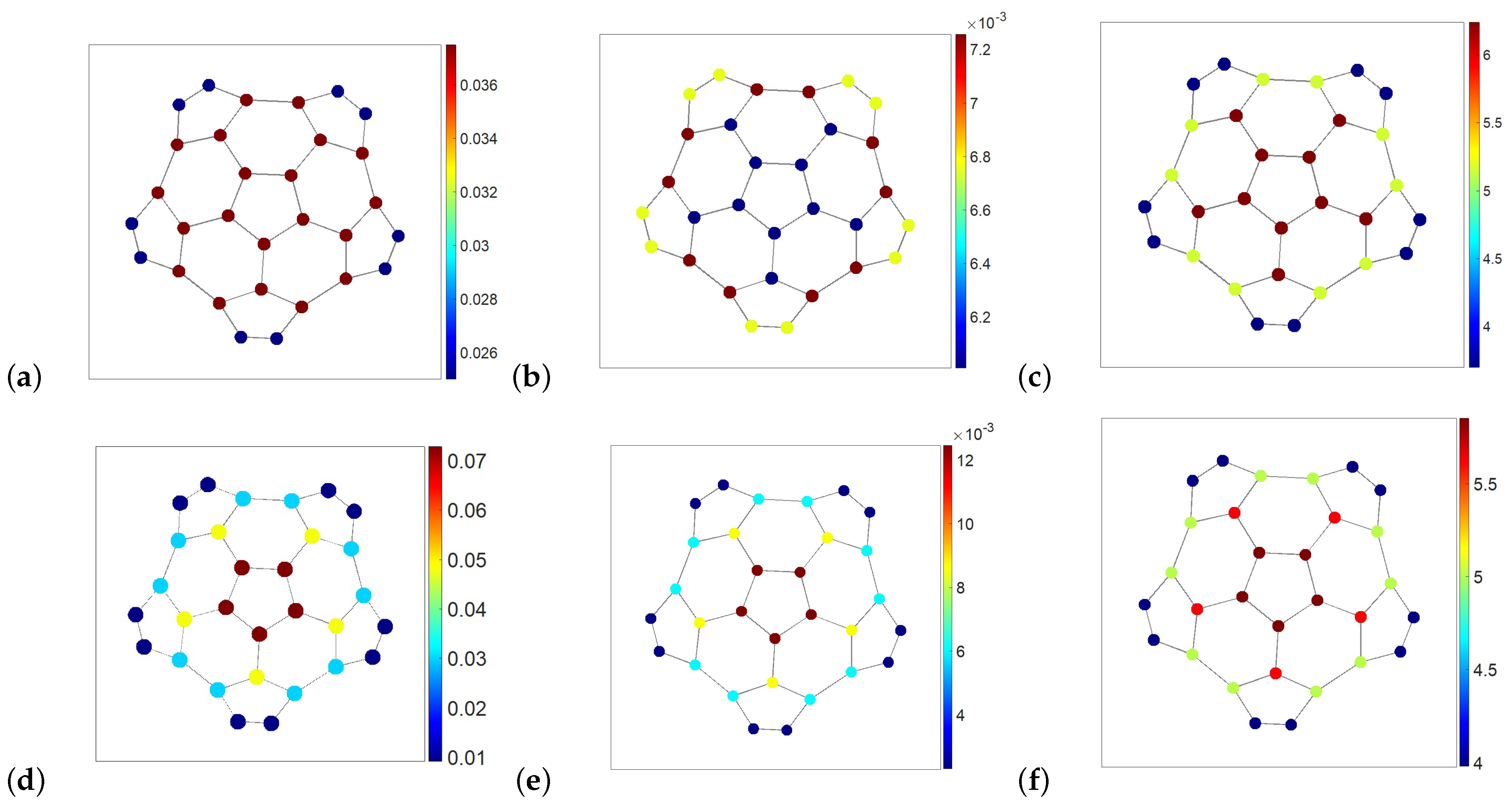
. In
Figure 4, we presented a buckle graph with nodes color-coded according to the node’s density, navigability, and strive potentials calculated for the different graph exploration strategies represented by the isotropic (
) and maximally anisotropic (
) random walks, respectively. Namely, in
Figure 4a–c, the graph nodes are color-coded with respect to the quantities calculated for the isotropic, first-order walks, in which a random walker chooses the next node equiprobably over all nearest neighbors. The corresponding node density defined with respect to
(see
Figure 4a) represents the node degree centrality: the better-connected nodes have a higher probability of hosting a random walker.
The navigability potential of nodes for the random walks
is shown in
Figure 4b. The nodes that have fewer neighbors, as well as those connected to them (located on graph’s boundary), are easy to navigate by isotropic random walks. On the contrary, the location of a walker over the better-connected nodes located at the graph center is less predictable. Conversely, the strive potential of nodes with respect to the random walks
presented in
Figure 4c is maximal for the central nodes of the graph (the longest neighborhood exploration time).
The node density with respect to the Ruelle–Bowen random walks of maximal anisotropy defined by the transition matrix
(
12) corresponds to the square root of the node’s eigenvector centrality (see
Figure 4d). The Ruelle–Bowen random walks are statistically confined to the graph center, hosting the lion’s share of available infinite paths but repelling from the graph boundaries. The confinement of anisotropic walks at the best structurally integrated part of the graph reveals itself by the fact that the magnitude of the node’s density at the graph center is as twice as high with respect to
than with respect to
and, vice versa, the Ruelle–Bowen random walkers are less probably found on the graph’s boundaries than those following isotropic random walks.
The navigability potential of nodes with respect to Ruelle–Bowen random walks
presented in
Figure 4e is dominated by the node’s density for anisotropic walks (the square root of the node’s eigenvector centrality) and enhanced by the effect of their confinement at the graph center. The appearance of anisotropic walks in the central part of the graph is more predictable than that on the graph boundary.
In contrast to isotropic random walks, the strive potential of nodes with respect to the Ruelle–Bowen random walks
is highest over the ring of five central nodes of the graph (see
Figure 4f). The neighborhood exploration time of the center by the Ruelle–Bowen random walks slightly exceeds five (steps), indicating that these walks are indeed statistically confined within the central ring.
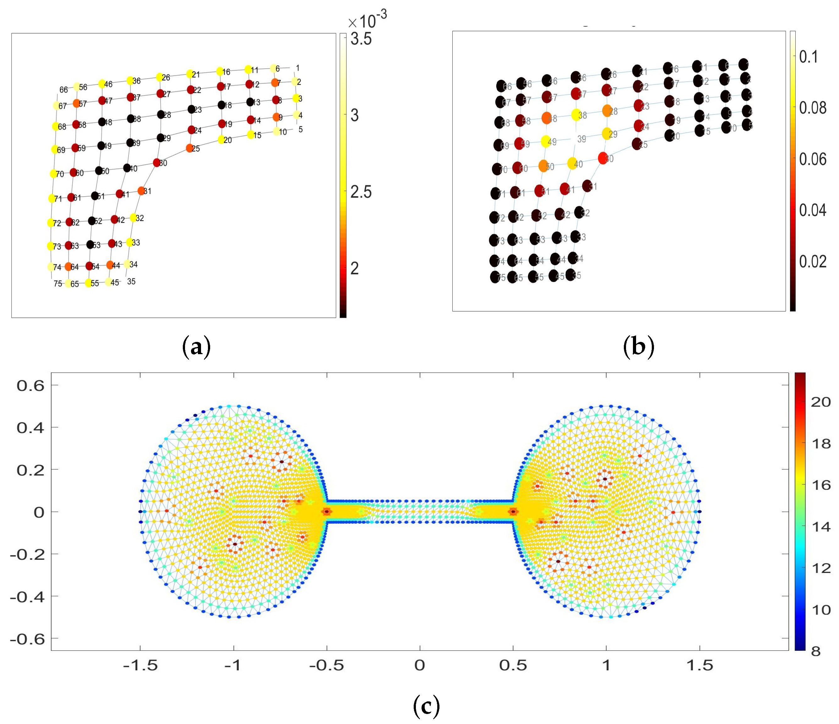
In
Figure 5a,b, we contrasted the navigability potentials of nodes in a membrane graph explored by isotropic random walks
(a) and by Ruelle–Bowen random walks
(b), respectively. Again, the isotropic walks are most predictable along the graph’s boundaries and at the membrane’s corners especially, but the location of walkers can hardly be predicted while in the central part of the graph. On the contrary, the navigability of the central nodes is highest if the graph is explored by Ruelle–Bowen random walks
due to the statistical confinement of anisotropic walks at the best structurally integrated part of the graph. Finally, in
Figure 5c, we have presented the strive potential of nodes (neighborhood’s exploration times) in a barbell graph explored by isotropic random walks
, and the nodes of the highest degree indeed generate the maximal strive for those walks.
As the expected node’s neighborhood exploration time serves as a statistical estimate of its neighborhood size,
, we may conclude that the navigation properties of the graph vertices are determined by the sizes of their neighborhoods with respect to the chosen graph exploration strategy. In particular, the navigability potential of a node as defined in (
20) is nothing else but the “specific” density of the vertex over the size of its neighborhood, viz.,
. This observation can be formulated as the following “uncertainty principle” for isotropic random walks in graphs:
the larger the neighborhood of a vertex, the less reliable the assumption that a random walker is at it. In
Figure 5c, the statistical neighborhoods of the best-connected nodes are highlighted in dark red and red as being characterized by the maximal strive magnitudes with respect to the isotropic random walks in the barbell graph. The anisotropic random walks are statistically confined within the best-integrated nodes of the graph, furthest from the graph’s boundaries and structural irregularities, and therefore these nodes are the most predictable of all.


