1. Introduction
Over the past few decades, attempts have been made to provide human-like commonsense reasoning to systems by acquiring vast knowledge about any domain. Humans are intuitively good at dealing with uncertainties and making meaningful inferences from incomplete, missing, and unstructured information. On the other hand, machines need precise information typically stored in a structured database and queried using a parsing strategy or well-defined rules. It is hard to rely on traditional relational data stores, as the massive influx of unstructured data and real-world information continuously evolve.
In recent years, knowledge graphs (KGs) have emerged as a flexible representation using the graph-based data model. They capture and integrate factual knowledge from diverse sources of data at a large scale in a way that machines conduct reasoning and inference over the graphs for downstream tasks such as question answering, making useful recommendations, etc., [
1].
The knowledge graph allows for postponing the schema definition, thus letting the data evolve more flexibly [
2]. A typical data unit in knowledge graphs is stored as entity–relationship–entity triplets, representing entities as nodes and relationships as the edges in a graph. The nodes are modeled to contain the knowledge or facts about the entities in the form of entity attributes. However, most existing systems used in answering a question over the knowledge graphs rely on static knowledge bases (KBs to train the knowledge graph question-answering (KGQA) model. These systems are trained offline with specific datasets and then deployed online to handle user queries. After deployment, they fail to learn from unseen new entities added to the graph. Thus, the problem faced by the knowledge graphs is the need for dynamic algorithms which can continuously learn and adapt to evolving data [
3].
Another challenge is the explainability and interpretation of the results when a query is posed to these evolving graphs. Question answering in knowledge graphs requires reasoning over multiple edges to arrive at the right answer and should have a tractable path to explain the new behavior [
4,
5]. A full explanation of the answer helps the users in their interaction with the system. For example, a query such as,
“Which paper author Amanda published in SIGIR conference?” needs multihop reasoning of the form,
and
to deduce the answer. Given the nature of this domain, if more papers, conferences, or authors are added in the future, the inference mechanisms need to be adaptable to the changes and interpretable to trace the new paths.
The state-of-the-art embedding-based neural network models for answering semantic queries consider only the candidate answer entities. They learn embeddings conditioned on neighboring entities and relations while being oblivious to the query relations and path. These methods help deduce the new facts but need more interpretation and logical reasoning of the answer [
6]. The alternative approach uses path-based methods including path ranking algorithms (PRAs) based on random walk [
7], DeepPath [
8] etc. These methods are highly interpretable but suffer from large search space issues [
9]. Moreover, they consider only a static snapshot and fail to learn from dynamically changing knowledge graphs [
10].
In this paper, we propose using the auction algorithms recently introduced in the paper [
11], to perform question answering in knowledge graphs. These algorithms are dynamic and can adapt to the changing environments in real time, making them suitable for offline and online training. They can help knowledge graphs to address the challenges of adaptability and interpretability.
The main auction path construction (APC) algorithm, to be discussed in
Section 3, computes paths (not necessarily the shortest) connecting an origin node to one or more destination nodes in a directed graph and uses node prices to guide the search for the path. The prices are initially chosen arbitrarily and are dynamically updated using a set of rules to be described later. When new entities are added or removed from the graph, the algorithm can dynamically adapt to the changing structure by reusing the prices for existing nodes and allocating arbitrary prices to the new nodes. The prices provide the means to “transfer knowledge”. The prices from previous searches can be used as initial prices for subsequent related searches, resulting in faster computation.
The auction algorithms provide full traceable paths and not just the single entity answer score. The full path can give the user a logical inference for the queries requiring multihop reasoning. Thus, the final answer constructed using our method is interpretable and provides an explainable answer. In particular, we can leverage the knowledge graph path relations, entity metadata, and attributes to add semantic information to the paths constructed by the auction algorithms.
The main contributions of the paper are as follows:
We propose a new method using auction algorithms for question answering in knowledge graphs.
We show that knowledge graphs can take advantage of the dynamic nature of auction algorithms.
Our results show that the computational efficiency of the search can be improved by reusing the prices that have been learned from previous queries.
Lastly, we leverage the entity metadata and path relations to construct an interpretable answer from the resulting path given by auction algorithms.
The paper is organized as follows. The next section describes related work.
Section 3 describes and explains the auction algorithms. The adaptation of auction algorithms in knowledge graphs for question answering is given in
Section 4.
Section 5 provides our experimental results and analysis.
Author Contributions
Conceptualization, G.A. and D.B.; methodology, G.A.; software, G.A.; validation, G.A. and D.B.; formal analysis, G.A.; investigation, G.A.; resources, G.A.; data curation, G.A.; writing—original draft preparation, G.A.; writing—review and editing, G.A., D.B. and H.L; visualization, G.A.; supervision, D.B. and H.L.; project administration, H.L.; funding acquisition, H.L. All authors have read and agreed to the published version of the manuscript.
Funding
This material is based upon work supported by the National Science Foundation under grant no. 2114789. Any opinions, findings, and conclusions or recommendations expressed in this material are those of the author(s) and do not necessarily reflect the views of the National Science Foundation.
Data Availability Statement
Not applicable.
Conflicts of Interest
The authors declare no conflict of interest.
Abbreviations
The following abbreviations are used in this manuscript:
| KG | knowledge graph |
| KGQA | knowledge graph question-answering system |
| KB | knowledge base |
| NER | named entity recognition |
| NLP | natural language processing |
References
- Kejriwal, M. Domain-Specific Knowledge Graph Construction; Springer: Berlin/Heidelberg, Germany, 2019. [Google Scholar]
- Hogan, A.; Blomqvist, E.; Cochez, M.; d’Amato, C.; Melo, G.D.; Gutierrez, C.; Kirrane, S.; Gayo, J.E.L.; Navigli, R.; Neumaier, S.; et al. Knowledge graphs. ACM Comput. Surv. CSUR 2021, 54, 1–37. [Google Scholar]
- Chen, Z.; Wang, Y.; Zhao, B.; Cheng, J.; Zhao, X.; Duan, Z. Knowledge graph completion: A review. IEEE Access 2020, 8, 192435–192456. [Google Scholar] [CrossRef]
- Saxena, A.; Tripathi, A.; Talukdar, P. Improving multi-hop question answering over knowledge graphs using knowledge base embeddings. In Proceedings of the 58th Annual Meeting of the Association for Computational Linguistics, Online, 5–10 July 2020; pp. 4498–4507. [Google Scholar]
- Geng, S.; Fu, Z.; Tan, J.; Ge, Y.; De Melo, G.; Zhang, Y. Path Language Modeling over Knowledge Graphsfor Explainable Recommendation. In Proceedings of the ACM Web Conference 2022, Lyon, France, 25–29 April 2022; pp. 946–955. [Google Scholar]
- Rossi, A.; Barbosa, D.; Firmani, D.; Matinata, A.; Merialdo, P. Knowledge graph embedding for link prediction: A comparative analysis. ACM Trans. Knowl. Discov. Data TKDD 2021, 15, 1–49. [Google Scholar] [CrossRef]
- Lao, N.; Mitchell, T.; Cohen, W. Random walk inference and learning in a large scale knowledge base. In Proceedings of the 2011 Conference on Empirical Methods in Natural Language Processing, Edinburgh, UK, 27–31 July 2011; pp. 529–539. [Google Scholar]
- Xiong, W.; Hoang, T.; Wang, W.Y. Deeppath: A reinforcement learning method for knowledge graph reasoning. arXiv 2017, arXiv:1707.06690. [Google Scholar]
- Lan, Y.; He, G.; Jiang, J.; Jiang, J.; Zhao, W.X.; Wen, J.R. Complex knowledge base question answering: A survey. IEEE Trans. Knowl. Data Eng. 2022. [Google Scholar] [CrossRef]
- Bhowmik, R.; Melo, G.D. Explainable link prediction for emerging entities in knowledge graphs. In Proceedings of the International Semantic Web Conference, Athens, Greece, 2–6 November 2020; Springer: Berlin/Heidelberg, Germany, 2020; pp. 39–55. [Google Scholar]
- Bertsekas, D.P. New Auction Algorithms for Path Planning, Network Transport, and Reinforcement Learning. arXiv 2022, arXiv:2207.09588. [Google Scholar]
- Nguyen, D.Q. An overview of embedding models of entities and relationships for knowledge base completion. arXiv 2017, arXiv:1703.08098. [Google Scholar]
- Palmonari, M.; Minervini, P. Knowledge graph embeddings and explainable AI. Knowl. Graphs Explain. Artif. Intell. Found. Appl. Chall. 2020, 47, 49. [Google Scholar]
- Bao, J.; Duan, N.; Yan, Z.; Zhou, M.; Zhao, T. Constraint-based question answering with knowledge graph. In Proceedings of the COLING 2016, the 26th International Conference on Computational Linguistics: Technical Papers, Osaka, Japan, 11–16 December 2016; pp. 2503–2514. [Google Scholar]
- Ren, H.; Dai, H.; Dai, B.; Chen, X.; Yasunaga, M.; Sun, H.; Schuurmans, D.; Leskovec, J.; Zhou, D. Lego: Latent execution-guided reasoning for multi-hop question answering on knowledge graphs. In Proceedings of the International Conference on Machine Learning, PMLR, Virtual, 18–24 July 2021; pp. 8959–8970. [Google Scholar]
- Das, R.; Dhuliawala, S.; Zaheer, M.; Vilnis, L.; Durugkar, I.; Krishnamurthy, A.; Smola, A.; McCallum, A. Go for a walk and arrive at the answer: Reasoning over paths in knowledge bases using reinforcement learning. arXiv 2017, arXiv:1711.05851. [Google Scholar]
- Fu, Z.; Xian, Y.; Gao, R.; Zhao, J.; Huang, Q.; Ge, Y.; Xu, S.; Geng, S.; Shah, C.; Zhang, Y.; et al. Fairness-aware explainable recommendation over knowledge graphs. In Proceedings of the 43rd International ACM SIGIR Conference on Research and Development in Information Retrieval, Virtual, 25–30 July 2020; pp. 69–78. [Google Scholar]
- Bertsekas, D.P. A Distributed Algorithm for the Assignment Problem; Lab. for Information and Decision Systems Working Paper; MIT: Cambridge, MA, USA, 1979. [Google Scholar]
- Bertsekas, D.P. Auction algorithms for network flow problems: A tutorial introduction. Comput. Optim. Appl. 1992, 1, 7–66. [Google Scholar] [CrossRef]
- Bertsekas, D. Network Optimization: Continuous and Discrete Models; Athena Scientific: Nashua, NH, USA, 1998; Volume 8. [Google Scholar]
- Dieci, L.; Walsh, J.D., III. The boundary method for semi-discrete optimal transport partitions and Wasserstein distance computation. J. Comput. Appl. Math. 2019, 353, 318–344. [Google Scholar] [CrossRef]
- Merigot, Q.; Thibert, B. Optimal transport: Discretization and algorithms. In Handbook of Numerical Analysis; Elsevier: Amsterdam, The Netherlands, 2021; Volume 22, pp. 133–212. [Google Scholar]
- Peyré, G.; Cuturi, M. Computational optimal transport: With applications to data science. Found. Trends Mach. Learn. 2019, 11, 355–607. [Google Scholar] [CrossRef]
- Lewis, M.; Bhosale, S.; Dettmers, T.; Goyal, N.; Zettlemoyer, L. Base layers: Simplifying training of large, sparse models. In Proceedings of the International Conference on Machine Learning, PMLR, Virtual, 18–24 July 2021; pp. 6265–6274. [Google Scholar]
- Bicciato, A.; Torsello, A. GAMS: Graph Augmentation with Module Swapping. In Proceedings of the ICPRAM, Virtual, 3–5 February 2022; pp. 249–255. [Google Scholar]
- Clark, A.; de Las Casas, D.; Guy, A.; Mensch, A.; Paganini, M.; Hoffmann, J.; Damoc, B.; Hechtman, B.; Cai, T.; Borgeaud, S.; et al. Unified scaling laws for routed language models. In Proceedings of the International Conference on Machine Learning, PMLR, Baltimore, MD, USA, 17–23 July 2022; pp. 4057–4086. [Google Scholar]
- Bertsekas, D.P. An auction algorithm for shortest paths. SIAM J. Optim. 1991, 1, 425–447. [Google Scholar] [CrossRef]
- Goyal, A.; Gupta, V.; Kumar, M. Recent named entity recognition and classification techniques: A systematic review. Comput. Sci. Rev. 2018, 29, 21–43. [Google Scholar] [CrossRef]
- Grishman, R.; Sundheim, B.M. Message understanding conference-6: A brief history. In Proceedings of the COLING 1996 Volume 1: The 16th International Conference on Computational Linguistics, Copenhagen, Denmark, 5–9 August 1996. [Google Scholar]
- Chiticariu, L.; Krishnamurthy, R.; Li, Y.; Reiss, F.; Vaithyanathan, S. Domain adaptation of rule-based annotators for named-entity recognition tasks. In Proceedings of the 2010 Conference on Empirical Methods in Natural Language Processing, Online, 9–11 October 2010; pp. 1002–1012. [Google Scholar]
- Karkaletsis, V.; Fragkou, P.; Petasis, G.; Iosif, E. Ontology based information extraction from text. In Knowledge-Driven Multimedia Information Extraction and Ontology Evolution: Bridging the Semantic Gap; Springer: Berlin/Heidelberg, Germany, 2011; pp. 89–109. [Google Scholar]
- Al-Moslmi, T.; Ocaña, M.G.; Opdahl, A.L.; Veres, C. Named entity extraction for knowledge graphs: A literature overview. IEEE Access 2020, 8, 32862–32881. [Google Scholar] [CrossRef]
- Nadeau, D.; Sekine, S. A survey of named entity recognition and classification. Lingvisticae Investig. 2007, 30, 3–26. [Google Scholar] [CrossRef]
- Vasiliev, Y. Natural Language Processing with Python and spaCy: A Practical Introduction; No Starch Press: San Francisco, CA, USA, 2020. [Google Scholar]
- Srihari, R.K.; Li, W.; Cornell, T.; Niu, C. Infoxtract: A customizable intermediate level information extraction engine. Nat. Lang. Eng. 2008, 14, 33–69. [Google Scholar] [CrossRef]
- Tran, H.N.; Takasu, A. Exploring scholarly data by semantic query on knowledge graph embedding space. In International Conference on Theory and Practice of Digital Libraries; Springer: Berlin/Heidelberg, Germany, 2019; pp. 154–162. [Google Scholar]
- Yih, S.W.t.; Chang, M.W.; He, X.; Gao, J. Semantic parsing via staged query graph generation: Question answering with knowledge base. In Proceedings of the Joint Conference of the 53rd Annual Meeting of the ACL and the 7th International Joint Conference on Natural Language Processing of the AFNLP, Beijing, China, 26–31 July 2015. [Google Scholar]
- Bast, H.; Haussmann, E. More accurate question answering on freebase. In Proceedings of the 24th ACM International on Conference on Information and Knowledge Management, Melbourne, Australia, 18–23 October 2015; pp. 1431–1440. [Google Scholar]
- Mahdisoltani, F.; Biega, J.; Suchanek, F. YAGO3: A knowledge base from multilingual wikipedias. In Proceedings of the 7th Biennial Conference on Innovative Data Systems Research, CIDR Conference, Asilomar, CA, USA, 13–16 January 2014. [Google Scholar]
- Sinha, A.; Shen, Z.; Song, Y.; Ma, H.; Eide, D.; Hsu, B.J.; Wang, K. An overview of microsoft academic service (mas) and applications. In Proceedings of the 24th International Conference on World Wide Web, Florence, Italy, 18–22 May 2015; pp. 243–246. [Google Scholar]
- Tran, H.N.; Takasu, A. Multi-Partition Embedding Interaction with Block Term Format for Knowledge Graph Completion. arXiv 2020, arXiv:2006.16365. [Google Scholar]
- Tran, H.N.; Takasu, A. MEIM: Multi-partition Embedding Interaction beyond Block Term Format for Efficient and Expressive Link Prediction. arXiv 2022, arXiv:2209.15597. [Google Scholar]
- Suchanek, F.M.; Kasneci, G.; Weikum, G. Yago: A core of semantic knowledge. In Proceedings of the 16th International Conference on World Wide Web, Banff, AB, Canada, 8–12 May 2007; pp. 697–706. [Google Scholar]
- Hoffman, R.R.; Mueller, S.T.; Klein, G.; Litman, J. Metrics for explainable AI: Challenges and prospects. arXiv 2018, arXiv:1812.04608. [Google Scholar]
- Agrawal, G. Auction Path Construction Algorithms in Knowledge Graphs. 2023. Available online: https://github.com/garima0106/KG-Auction.git (accessed on 12 June 2023).
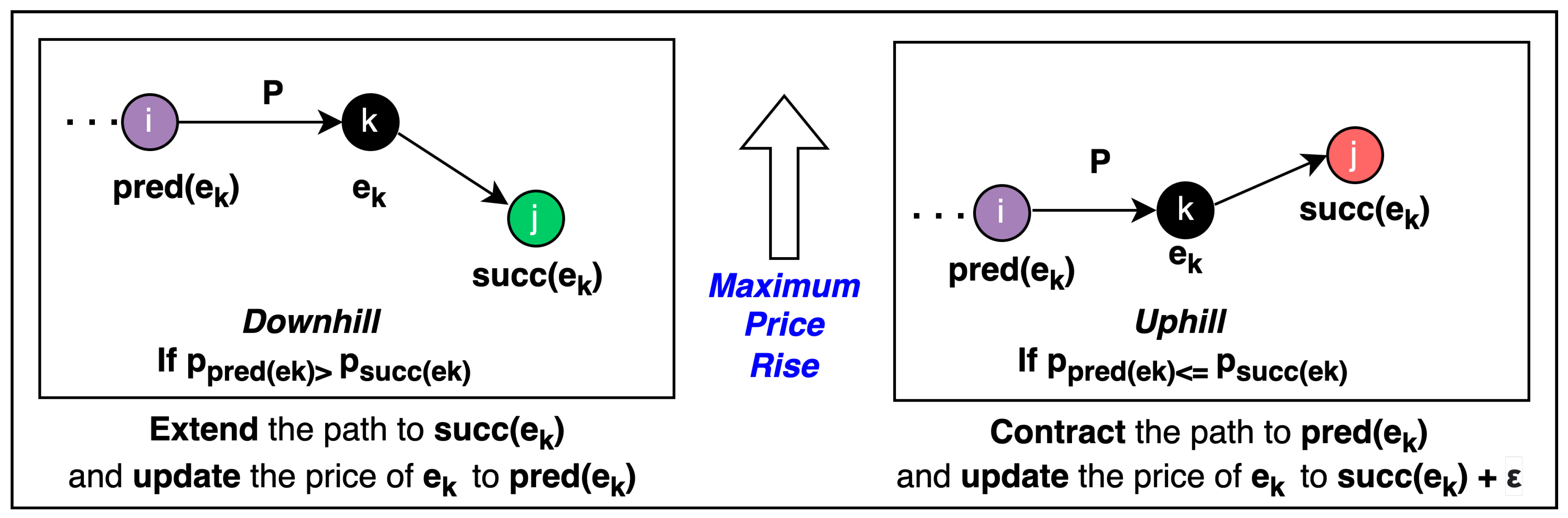
Figure 1.
Figure showing the price update and raising the price to the maximum possible level. In case of extension, the algorithm maintains the maximum possible level making the predecessor arc level. In the case of a contraction, it raises the price of to the maximum possible level, making the arc uphill.
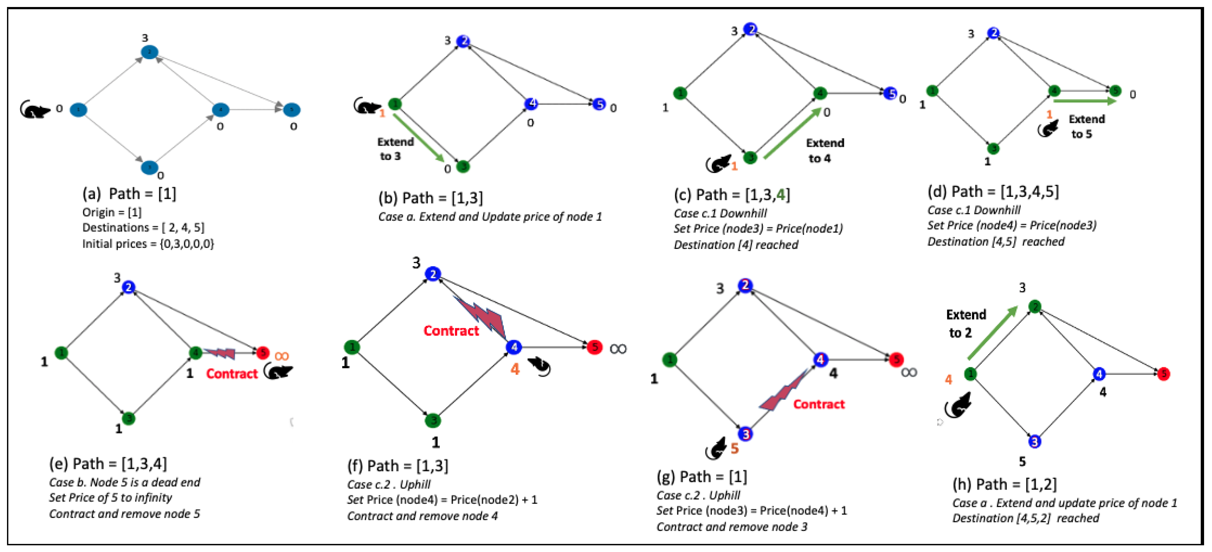
Figure 2.
The figure shows the APC traversal on a five-node graph. The initial prices are arbitrarily chosen as . The origin node is given as , with three destination nodes . The algorithm chooses to extend or contract and update the price as per the given rules. The prices after the update in each iteration are shown against each node in the figure.
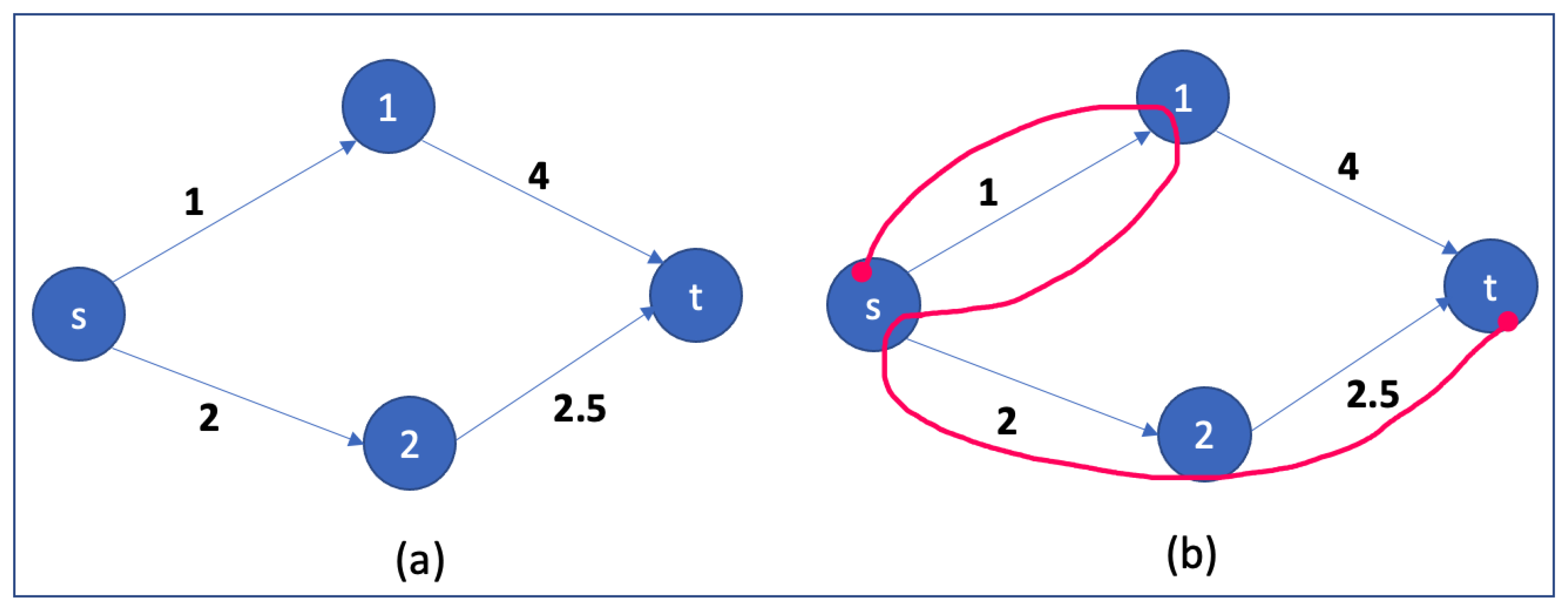
Figure 3.
The figure shows the AWPC traversal on a four-node graph. The initial prices are arbitrarily chosen as and edge weights as (a). The origin node is given as , with the destination node as . The algorithm chooses to extend or contract and update the price per the given rules. The path chosen by AWPC for is shown in (b).
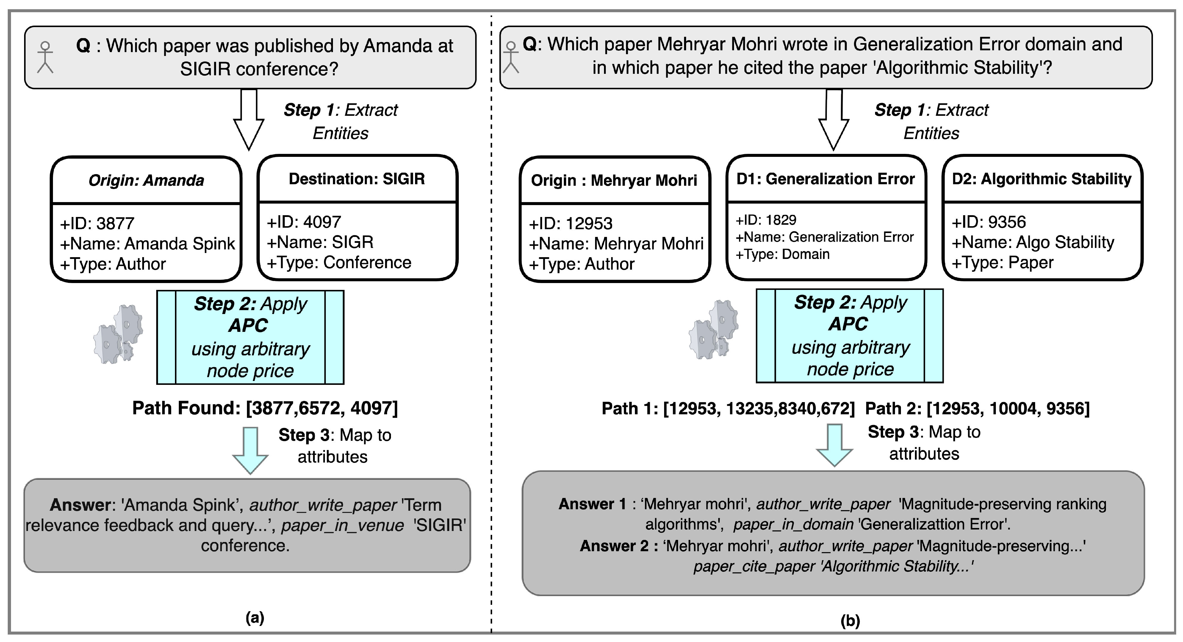
Figure 4.
The figure illustrates the step-wise method to answer queries. (a) The single destination query and (b) the query with two parts, i.e., multiple destinations.
Figure 5.
The figure illustrates the mapping of path nodes to entity attributes and edge relations to build an explainable answer.
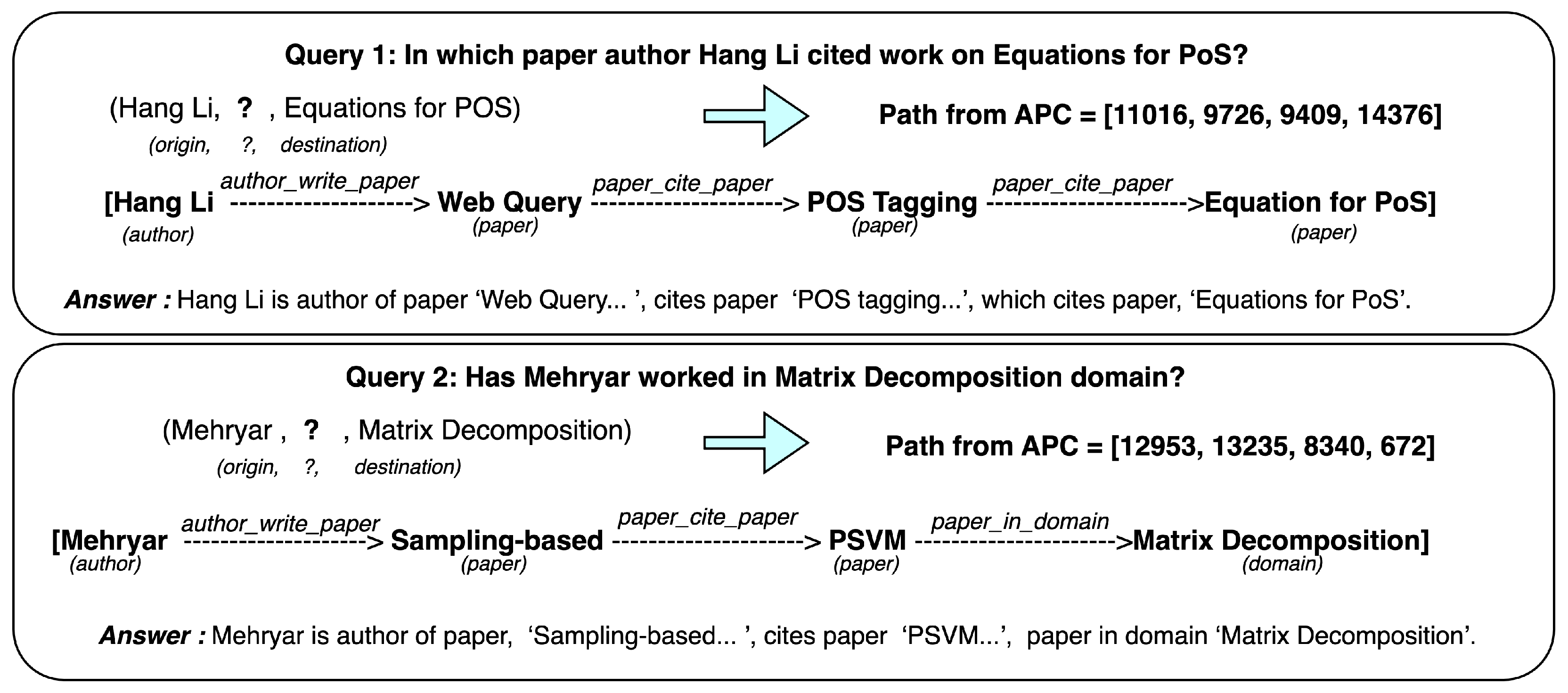
Figure 6.
Explainable paths given by our method in question answering for KG20C dataset.
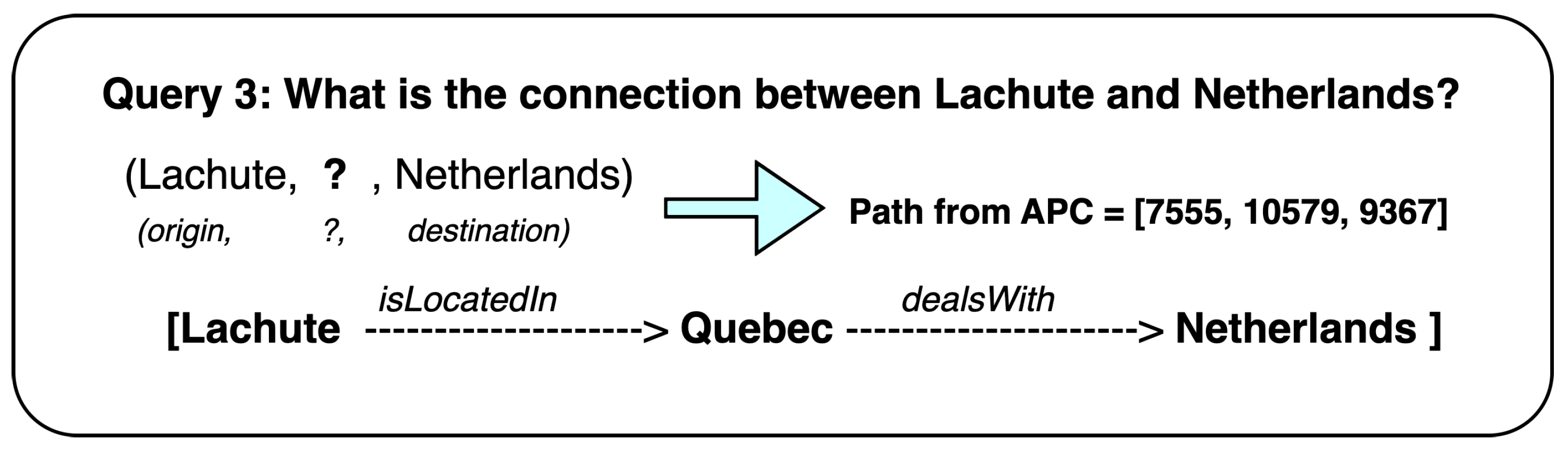
Figure 7.
Explainable paths for the query made to the YAGO3-10 dataset.
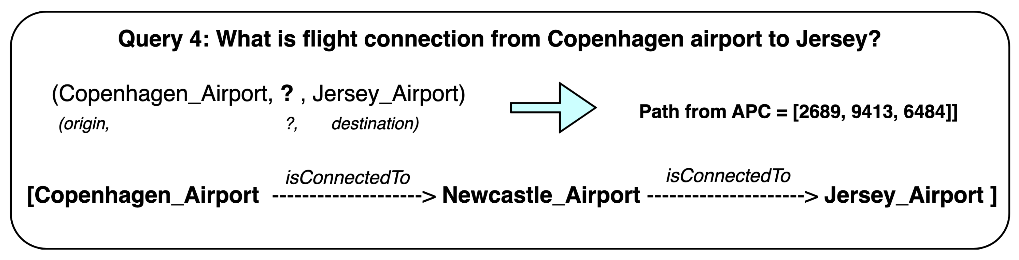
Figure 8.
Explainable path from another query from the YAGO3-10 dataset.
Table 1.
KG20C Triple dataset stats.
| Author | Paper | Conference | Domain | Affiliation | Entities | Relations | Edges |
|---|
| 8680 | 5047 | 20 | 1923 | 692 | 16,362 | 5 | 55,607 |
Table 2.
Experimental Setup.
| Algo | S.No. | Settings | Observations |
|---|
| APC | 1 | Initial Price as | Algorithm was relatively stable, and the resulting paths matched the ground truth. |
| 2 | Reusing Prices from (1) | Number of iterations reduced by . Resulting paths were the same as those in (1). |
| 3 | Random Prices and Stress Testing | Random prices given between 100 and 1000. Higher iterations. Most Paths were the same and gave longer paths for some queries. |
| 4 | Reusing Prices from (3) | Relatively stable. Iterations in (4) much fewer than those in (3) but higher or the same as those in (2). |
| AWPC | 5 | Edge Weights as | edge weights results should match the first four settings using APC; validation step. |
| 6 | Edge Weights as | Same paths; greater or equal number of iterations as in (2). |
| 7 | Random Weights | Unstable with random weights between −10 and 10. Iterations increased by almost two times, with not much change in the paths. |
| 8(a) | Weights as per “Query Semantics” (S:0,W:1) | Edges with strong match in query given weights and the remaining edges (weak) given “1”; no significant change in iterations. |
| 8(b) | (S:0,M:3,W:6) Prices Reused from an Initial Price of “0” | Paths were same or shorter, and iterations were fewer or the same as in (2). |
Table 3.
Number of Iterations for sample queries.
| Query | Price | EW = 1 | EW = [−10, 10] | EW(S:0,W:1) | EW(S:0,M:3,W:6) |
|---|
| In which paper did Hang-Li cite paper on “Equations for PoS”? | Initial price = 0 | 353 | 630 | 347 | 76 |
| In which paper author Fredric cited the paper on “Equations for PoS”? | Reusing prices | 2 | 32 | 2 | 2 |
| Which paper in “Clustering query” cites work on “Equations for PoS”? | Reusing prices | 3 | 13 | 3 | 3 |
Table 4.
Comparison of APC with the Embedding Method.
| Model | Prediction | Multihop Queries | Explainability | Training |
|---|
| Embedding(MEI) | Hits@10 < 70% | Not supported | Candidate entity score | Offline |
| APC | Matches ground truth | Supported | Gives full path | Both offline and online |
Table 5.
Comparison of the APC with the Dijkstra Algorithm.
| Criteria | APC | Dijkstra |
|---|
| Q1: “If Amanda has worked in cluster analysis domain?” | Path = [3877, 6572, 7780, 1119] | Path = [3877, 6572, 7780, 1119] |
| Q2: “If Mehryar Mohri has paper in COLT conference?” | Path = [12,953, 4459, 7868, 4117] suboptimal path | Path = [12,953, 4459, 4117], gives the shortest path |
| Explainability | Yes | Yes |
| Learn from Past Query | Yes | No |
| Computational Efficiency | More efficient for large scale graph | Computationally expensive for large scale |
| Adaptability to change | Dynamically evolves | Takes static snapshot of graph |
| Model Training | Both online and offline | Offline only |
Table 6.
Summary of Experiments and Results.
| Evaluation Criteria | APC (and AWPC) |
|---|
| Prediction Accuracy | Resulting paths match the ground truth |
| Evolving Knowledge Graph with Emerging Entities | Dynamically adapts to newly added entities |
| Explainable Reasoning and Interpretability | Returns traceable paths |
| Computational Efficiency | Reduced iterations on reusing node price |
| Multihop Queries | Supported |
| Queries with Multiple Destinations | Supported |
| Disclaimer/Publisher’s Note: The statements, opinions and data contained in all publications are solely those of the individual author(s) and contributor(s) and not of MDPI and/or the editor(s). MDPI and/or the editor(s) disclaim responsibility for any injury to people or property resulting from any ideas, methods, instructions or products referred to in the content. |
© 2023 by the authors. Licensee MDPI, Basel, Switzerland. This article is an open access article distributed under the terms and conditions of the Creative Commons Attribution (CC BY) license (https://creativecommons.org/licenses/by/4.0/).


