
A Single-Product Multi-Period Inventory Routing Problem under Intermittent Demand


Abstract
:1. Introduction
- (a)
- We focus on the problem of an IRP with intermittent demand patterns (IDIRP) and expand the scope of IRP research.
- (b)
- We introduce the lateral transshipment strategy into an IDIRP to cope with the demand fluctuations of intermittent patterns.
- (c)
- We develop an MIP model for the IDIRP and improve the operators of the ALNS algorithm to enhance the solution efficiency.
2. Literature Review
3. Model
- (1)
- The central warehouse inventory can meet the demand of all customers for all periods, and stock-outs are not allowed.
- (2)
- The central warehouse replenishes the same product to the customer without considering the cost and space impact brought by the heterogeneity of the product to the vehicle transportation.
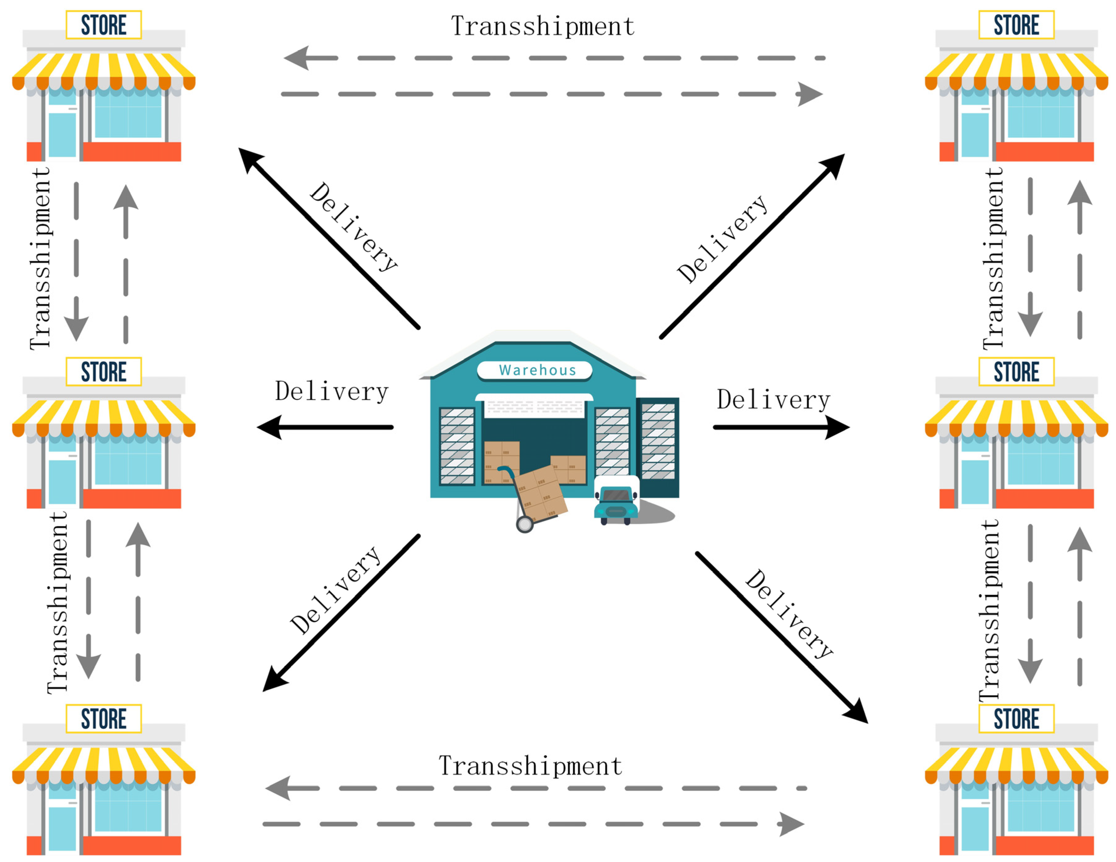
- (3)
- Lateral transshipment is only initiated by customers and can only be conducted between customers without considering the central warehouse.
- (4)
- In replenishment and lateral transshipment, only the impact of distance on cost is considered, and the difference arising from vehicle loads is not considered.
- (5)
- The unit cost of transshipment provided by third-party transportation service providers is lower than the unit cost of distribution by the company’s own vehicles.
3.1. Inventory Routing Model with Transshipment
3.1.1. Inventory Routing Model for the Planning Period
3.1.2. Lateral Transshipment Model in the Replenishment Cycle
4. Adaptive Large-Neighborhood Search Algorithm
- (1)
- Initial solution generation: an initial solution is generated according to the characteristics of the problem. The initial solution can be generated in greedy approaches, random ways, and heuristic algorithms. Additionally, some parameters of the algorithm are initialized, such as the weights of the operators and the corresponding scores.
- (2)
- Neighborhood search operation: choose a set of destroy and repair operators; the solution is destroyed to obtain a new solution and subsequently a repair operation is conducted on it to obtain the current solution.
- (3)
- Acceptance or rejection strategy: the simulated annealing algorithm is generally used to control whether the current solution is accepted or not, followed by judging whether the termination condition is satisfied; if not, proceed to step (4).
- (4)
- Neighborhood update: the weights and scores of the operators are updated according to the quality of the current solution.
- (5)
- Algorithm termination conditions: algorithm termination conditions are generally set in terms of running time and a specified number of iterations.
| Algorithm 1: The structure of the ALNS |
 |
4.1. Initial Solution Generation
4.2. Initial Solution Generation
- (1)
- Random removal
- (2)
- Worst removal
- (3)
- Shaw removal
- (4)
- Route removal
- (5)
- Neighborhood removal
- (6)
- Demand-based removal
- (7)
- Greedy insertion
- (8)
- Regret insertion
- (9)
- Random insertion
- (10)
- Sequential insertion
- (11)
- Swap insertion
4.3. Operator Selection and Weight Adjustment
4.4. Acceptance Criteria and Termination Conditions
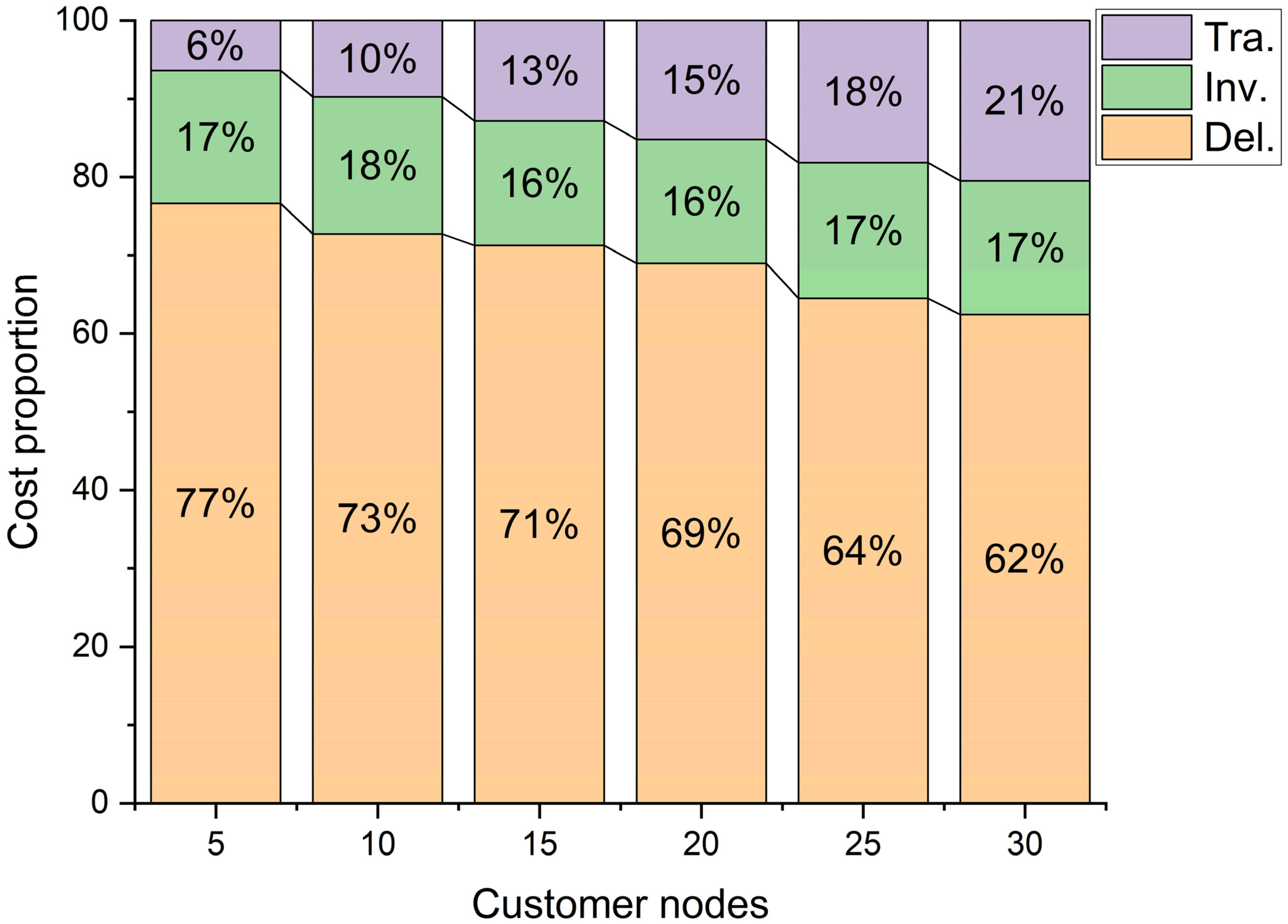
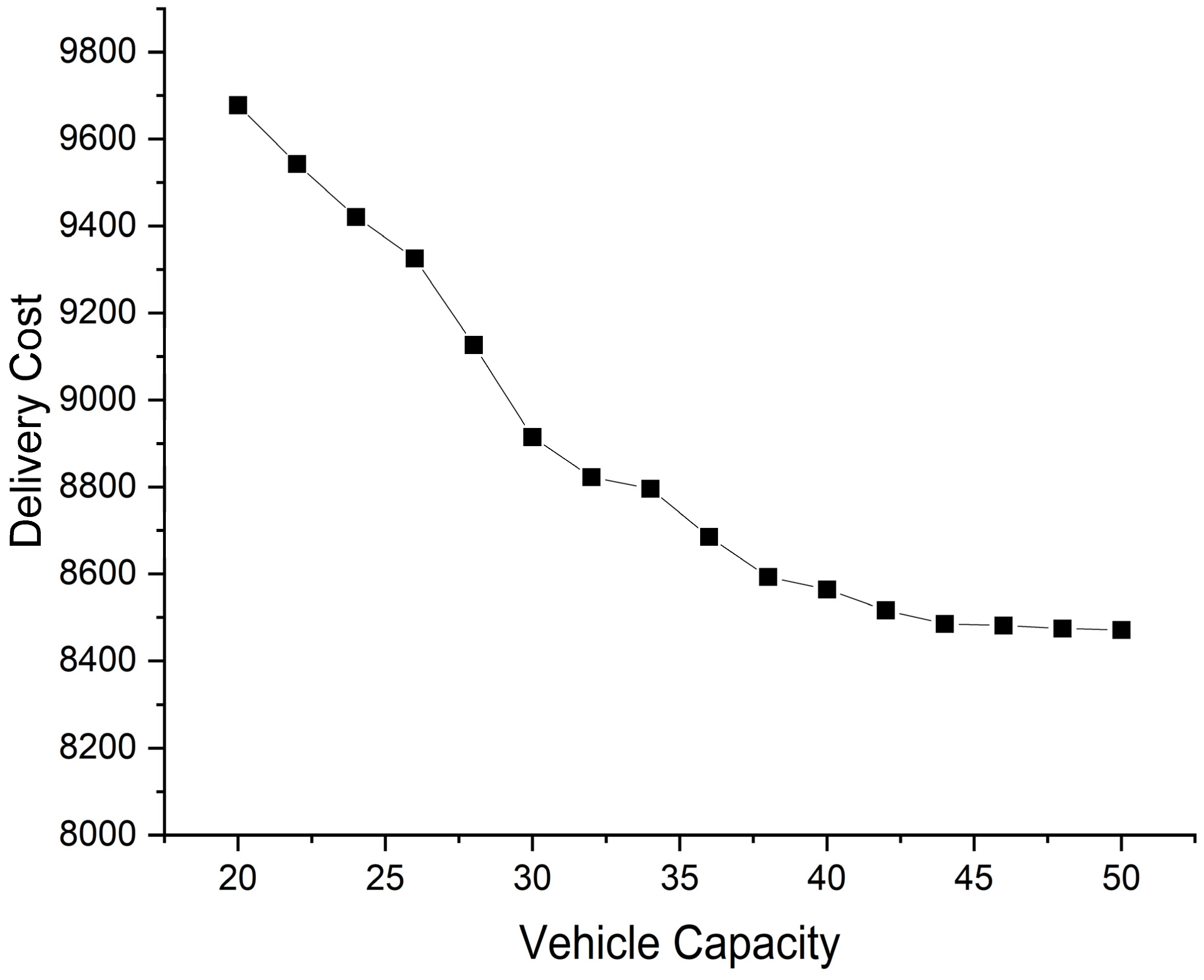
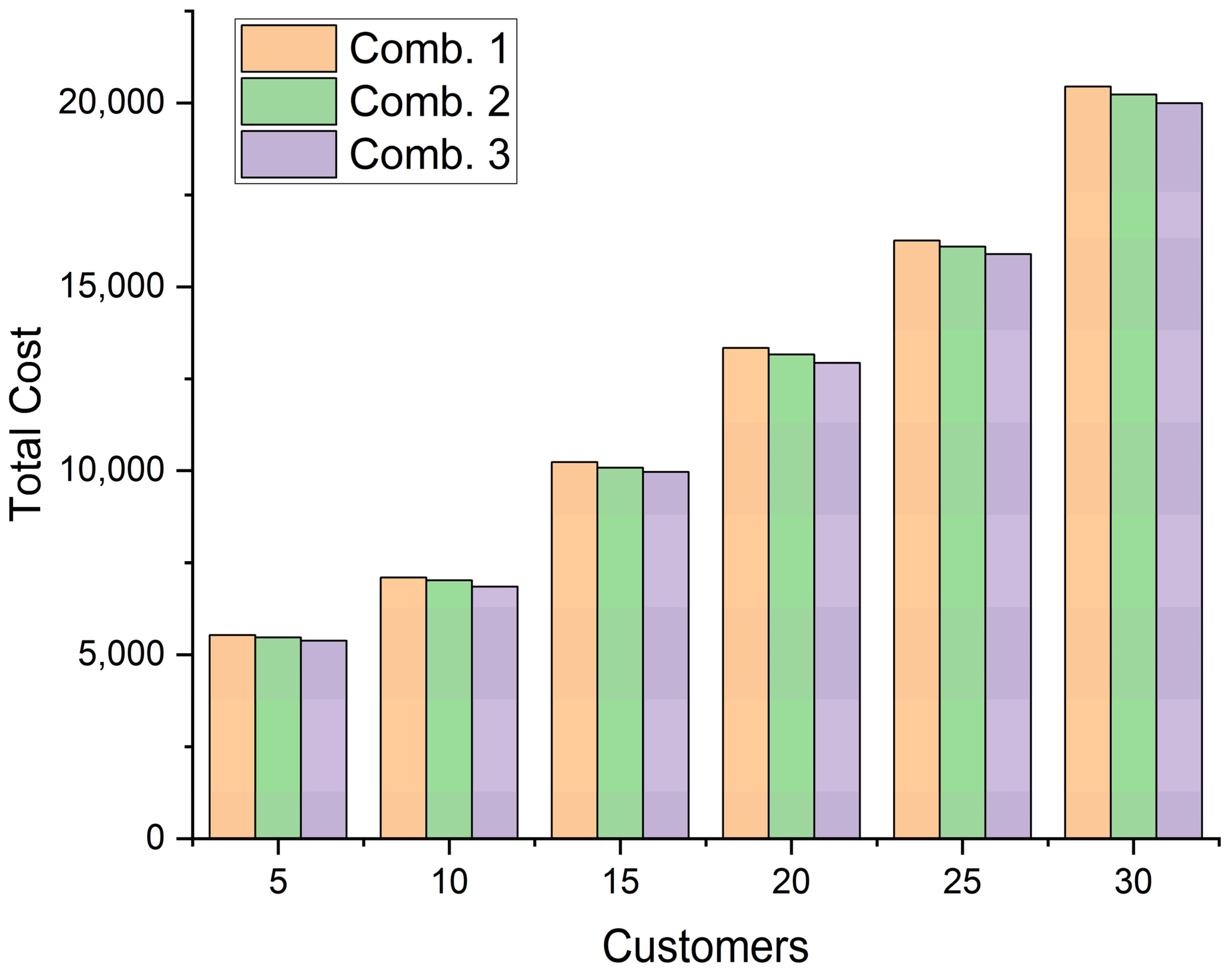
5. Case Study
6. Conclusions
Author Contributions
Funding
Data Availability Statement
Conflicts of Interest
Abbreviations
| Symbol | Meaning |
| Sets | |
| Set of all nodes, | |
| Set of all arcs, | |
| Central warehouse, | |
| Set of all customer nodes, | |
| Set of periods, | |
| Set of vehicles, | |
| Parameters | |
| Unit inventory cost in the central warehouse | |
| Unit inventory cost in customers | |
| Delivery cost per unit distance | |
| Transshipment cost per unit distance | |
| Inventory capacity of customers, | |
| Capacity of vehicles | |
| Distance between node I and j | |
| Variables | |
| The actual demand of node i at period t, | |
| At period t, the vehicle k visits node j after visiting node i, | |
| The number of goods transferred from node i to node j at period t, | |
| The inventory level of node i at the beginning of period t, | |
| The number of goods transported by vehicle k from the central warehouse to node i at time t, | |
| Dummy variables for sub-loop elimination | |
References
- Biuki, M.; Kazemi, A.; Alinezhad, A. An integrated location-routing-inventory model for sustainable design of a perishable products supply chain network. J. Clean. Prod. 2020, 260, 120842. [Google Scholar] [CrossRef]
- Dey, B.K.; Seok, H. Intelligent inventory management with autonomation and service strategy. J. Intell. Manuf. 2022, 1–24. [Google Scholar] [CrossRef]
- Mandal, B.; Dey, B.K.; Khanra, S.; Sarkar, B. Advance sustainable inventory management through advertisement and trade-credit policy. RAIRO-Oper. Res. 2021, 55, 261–284. [Google Scholar] [CrossRef]
- Dalalah, D.; Al-Araidah, O. Dynamic decentralised balancing of CONWIP production systems. Int. J. Prod. Res. 2010, 48, 3925–3941. [Google Scholar] [CrossRef]
- Wu, S.N.; Liu, Q.; Zhang, R.Q. The Reference Effects on a Retailer’s Dynamic Pricing and Inventory Strategies with Strategic Consumers. Oper. Res. 2015, 63, 1320–1335. [Google Scholar] [CrossRef]
- Williams, T.M. Stock Control with Sporadic and Slow-Moving Demand. J. Oper. Res. Soc. 1984, 35, 939–948. [Google Scholar] [CrossRef]
- Syntetos, A.A.; Boylan, J.E.; Croston, J.D. On the categorization of demand patterns. J. Oper. Res. Soc. 2005, 56, 495–503. [Google Scholar] [CrossRef]
- Turkmen, A.; Januschowski, T.; Wang, Y.Y.; Cemgil, A. Intermittent Demand Forecasting with Renewal Processes. arXiv 2010, arXiv:2010.01550. [Google Scholar]
- Wu, W.T.; Zhou, W.; Lin, Y.; Xie, Y.Q.; Jin, W.Z. A hybrid metaheuristic algorithm for location inventory routing problem with time windows and fuel consumption. Expert Syst. Appl. 2021, 166, 114034. [Google Scholar] [CrossRef]
- Olgun, M.O.; Aydemir, E. A new cooperative depot sharing approach for inventory routing problem. Ann. Oper. Res. 2023, 307, 417–441. [Google Scholar] [CrossRef]
- Dantzig, G.B.; Ramser, J.H. The Truck Dispatching Problem. Manag. Sci. 1959, 6, 80–91. [Google Scholar] [CrossRef]
- Alkaabneh, F.; Diabat, A. A multi-objective home healthcare delivery model and its solution using a branch-and-price algorithm and a two-stage meta-heuristic algorithm. Transp. Res. Part C Emerg. Technol. 2023, 147, 103838. [Google Scholar] [CrossRef]
- Mousavi, R.; Salehi-Amiri, A.; Zahedi, A.; Hajiaghaei-Keshteli, M. Designing a supply chain network for blood decomposition by utilizing social and environmental factor. Comput. Ind. Eng. 2021, 160, 107501. [Google Scholar] [CrossRef]
- Yin, Y.; Liu, X.; Chu, F.; Wang, D. An exact algorithm for the home health care routing and scheduling with electric vehicles and synergistic-transport mode. Ann. Oper. Res. 2023, 1–36. [Google Scholar] [CrossRef]
- Bell, W.J.; Dalberto, L.M.; Fisher, M.L.; Greenfield, A.J.; Jaikumar, R.; Kedia, P.; Mack, R.G.; Prutzman, P.J. Improving the Distribution of Industrial Gases with an On-Line Computerized Routing and Scheduling Optimizer. Interfaces 1983, 13, 4–23. [Google Scholar] [CrossRef]
- Abdelmaguid, T.F.; Dessouky, M.M.; Ordóñez, F. Heuristic approaches for the inventory-routing problem with backlogging. Comput. Ind. Eng. 2009, 56, 1519–1534. [Google Scholar] [CrossRef]
- Raa, B.; Aghezzaf, E.-H. A practical solution approach for the cyclic inventory routing problem. Eur. J. Oper. Res. 2009, 192, 429–441. [Google Scholar] [CrossRef]
- Geiger, M.J.; Sevaux, M. On the Use of Reference Points for the Biobjective Inventory Routing Problem. arXiv 2011, arXiv:1109.3094. [Google Scholar]
- Cárdenas-Barrón, L.; González-Velarde, J.L.; Treviño-Garza, G.; Garza-Nuñez, D. Heuristic algorithm based on reduce and optimize approach for a selective and periodic inventory routing problem in a waste vegetable oil collection environment. Int. J. Prod. Econ. 2019, 211, 44–59. [Google Scholar] [CrossRef]
- Lefever, W.; Aghezzaf, E.; Hadj-Hamou, K.; Penz, B. Analysis of an improved branch-and-cut formulation for the Inventory-Routing Problem with Transshipment. Comput. Oper. Res. 2018, 98, 137–148. [Google Scholar] [CrossRef]
- Coelho, L.C.; Maio, A.D.; Laganà, D. A variable MIP neighborhood descent for the multi-attribute inventory routing problem. Transp. Res. Part E Logist. Transp. Rev. 2020, 144, 102137. [Google Scholar] [CrossRef]
- Rayat, F.; Musavi, M.; Bozorgi-Amiri, A. Bi-objective reliable location-inventory-routing problem with partial backordering under disruption risks: A modified AMOSA approach. Appl. Soft Comput. 2017, 59, 622–643. [Google Scholar] [CrossRef]
- Soysal, M.; Bloemhof-Ruwaard, J.; Haijema, R.; Vorst, J.G.V.D. Modeling a green inventory routing problem for perishable products with horizontal collaboration. Comput. Oper. Res. 2018, 89, 168–182. [Google Scholar] [CrossRef]
- Ji, Y.; Du, J.H.; Han, X.Y.; Wu, X.Q.; Huang, R.P.; Wang, S.L.; Liu, Z.M. A mixed integer robust programming model for two-echelon inventory routing problem of perishable products. Physica A 2020, 548, 124481. [Google Scholar] [CrossRef]
- Achamrah, F.E.; Riane, F.; Limbourg, S. Spare parts inventory routing problem with transshipment and substitutions under stochastic demands. Appl. Math. Model. 2022, 101, 309–331. [Google Scholar] [CrossRef]
- Ortega, E.; Doerner, K. A sampling-based matheuristic for the continuous-time stochastic inventory routing problem with time-windows. Comput. Oper. Res. 2023, 152, 106129. [Google Scholar] [CrossRef]
- Ropke, S.; Pisinger, D. An Adaptive Large Neighborhood Search Heuristic for the Pickup and Delivery Problem with Time Windows. Transp. Sci. 2006, 40, 455–472. [Google Scholar] [CrossRef] [Green Version]
- Shaw, P. Using Constraint Programming and Local Search Methods to Solve Vehicle Routing Problems. In Proceedings of the Principles and Practice of Constraint Programming—CP98: 4th International Conference, CP98, Pisa, Italy, 26–30 October 1998. [Google Scholar]
- Coelho, L.C.; Cordeau, J.-F.; Laporte, G. Consistency in multi-vehicle inventory-routing. Transp. Res. Part C Emerg. Technol. 2012, 24, 270–287. [Google Scholar] [CrossRef]
- Coelho, L.C.; Cordeau, J.-F.; Laporte, G. The inventory-routing problem with transshipment. Comput. Oper. Res. 2012, 39, 2537–2548. [Google Scholar] [CrossRef]
- Adulyasak, Y.; Cordeau, J.-F.; Jans, R. Optimization-Based Adaptive Large Neighborhood Search for the Production Routing Problem. Transp. Sci. 2014, 48, 20–45. [Google Scholar] [CrossRef]
- Alkaabneh, F.; Shehadeh, K.S.; Diabat, A. Routing and resource allocation in non-profit settings with equity and efficiency measures under demand uncertainty. Transp. Res. Part C Emerg. Technol. 2023, 149, 104023. [Google Scholar] [CrossRef]
- Demir, E.; Bektaş, T.; Laporte, G. An adaptive large neighborhood search heuristic for the Pollution-Routing Problem. Eur. J. Oper. Res. 2012, 223, 346–359. [Google Scholar] [CrossRef]
- Potvin, J.-Y.; Rousseau, J.-M. A parallel route building algorithm for the vehicle routing and scheduling problem with time windows. Eur. J. Oper. Res. 1993, 66, 331–340. [Google Scholar] [CrossRef]


| Reference | Period Type | Demand Type | Commodity Type | Fleet Composition | Solution Method |
|---|---|---|---|---|---|
| Cárdenas-Barrón et al. [19] | Multiple | Deterministic | Single | Homogeneous | Heuristics |
| Lefever et al. [20] | Multiple | Deterministic | Single | Homogeneous | Exact |
| Coelho et al. [21] | Multiple | Deterministic | Multiple | Heterogeneous | Exact |
| Rayat et al. [22] | Multiple | Stochastic | Multiple | Heterogeneous | Metaheuristics |
| Soysal et al. [23] | Multiple | Stochastic | Multiple | Homogeneous | CPLEX |
| Ji et al. [24] | Single | Stochastic | Single | Homogeneous | Gurobi |
| Achamrah et al. [25] | Multiple | Stochastic | Multiple | Homogeneous | Approximation |
| Ortega and Doerner [26] | Multiple | Fuzzy | Multiple | Homogeneous | Metaheuristics |
| This work | Multiple | Intermittent | Multiple | Homogeneous | Metaheuristics |
| Parameter | Description | Value | Unit |
|---|---|---|---|
| O | Number of central warehouses | 1 | - |
| P | Number of products | 1 | - |
| Number of customer nodes | 5, 10, 15, 20, 25, 30 | - | |
| Customer point coordinates | ([0, 100], [0, 100]) | - | |
| Customer distance | km | ||
| Periods | 3 | day | |
| Number of vehicles | [1, 10] | - | |
| Unit inventory cost in the central warehouse | 2 | dollar | |
| Unit inventory cost in customers | 4 | dollar | |
| Delivery cost per unit distance | 5 | dollar | |
| Transshipment cost per unit distance | 3 | dollar | |
| C | Capacity of vehicles | 30 | item |
| Capacity of customers, | [3, 8] | item |
| Parameter | Value | Description |
|---|---|---|
| 0.7 | Shaw removal operator, distance correlation weights between client nodes | |
| 0.2 | Shaw removal operator, customer demand quantity relevance weights | |
| 0.1 | Shaw removal operator, customer inventory capacity correlation weights | |
| 0.8 | Response factors in roulette strategy |
| Type | Route | Delivery Costs | Inventory Costs | Transshipment Costs | Total Cost | Time/s | |
|---|---|---|---|---|---|---|---|
| Day one | Delivery | 0-2-8-1-6-0 | 1375 | 396 | - | - | - |
| Transshipment | 3-5-4 | - | - | 318 | - | - | |
| Day two | Delivery | 0-7-9-4-10-0 | 1140 | 492 | - | - | - |
| Transshipment | 6-8 | - | - | 129 | - | - | |
| Day three | Delivery | 0-8-4-7-9-2-0 | 1810 | 312 | - | - | - |
| Transshipment | 5-3-1 | - | - | 222 | - | - | |
| Total | 4325 | 1200 | 669 | 6194 | 83 |
| Type | Route | Delivery Costs | Inventory Costs | Transshipment Costs | Total Cost | Time/s | |
|---|---|---|---|---|---|---|---|
| Day one | Delivery | 0-1-9-11-15-14-17-0, 0-12-2-8-5-4-0, 0-19-3-6-7-0 | 3635 | 632 | - | - | - |
| Transshipment | 13-10-16 | - | - | 645 | - | - | |
| Day two | Delivery | 0-8-2-9-7-16-0, 0-3-5-12-14-0, 0-11-17-19-1-2-0 | 2815 | 686 | - | - | - |
| Transshipment | 6-4-15 | - | - | 771 | - | - | |
| Day three | Delivery | 0-13-2-18-11-12-3-0, 0-7-1-15-19-0, 0-4-16-17-5-0 | 2465 | 728 | - | - | - |
| Transshipment | 2-6-20 | - | - | 552 | - | - | |
| Total | 8915 | 2046 | 1968 | 12,929 | 237 |
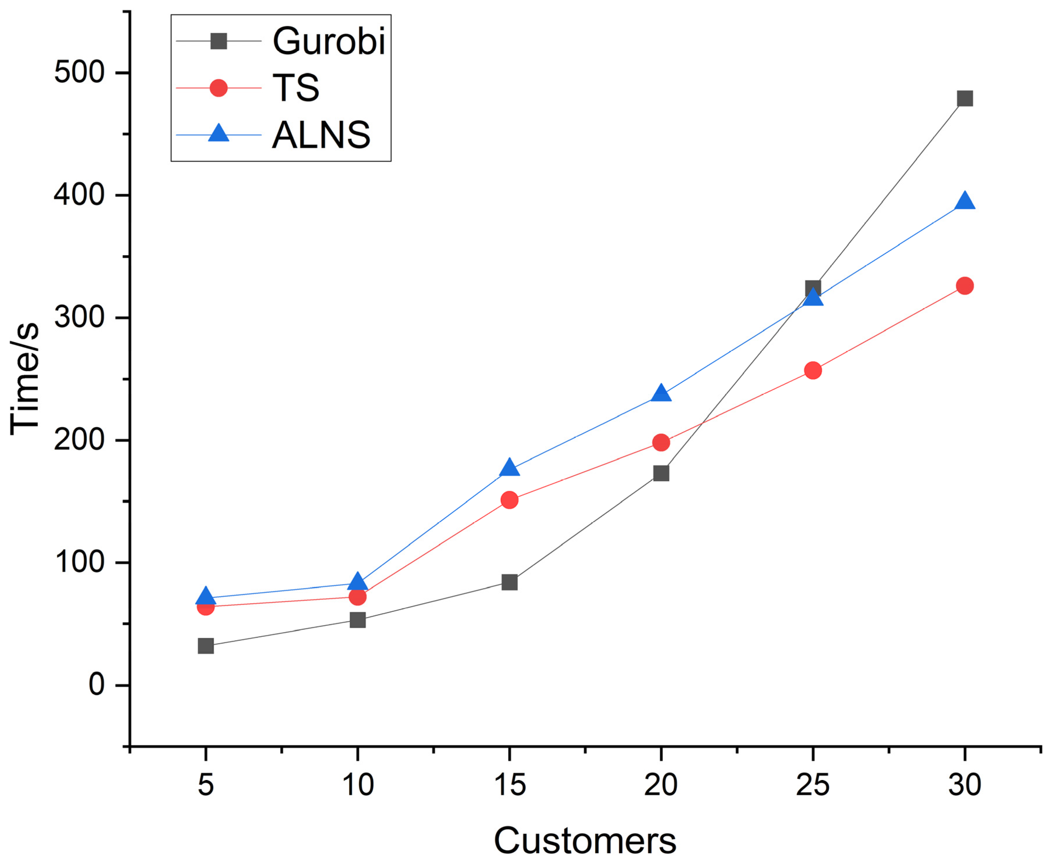
| Nodes | Gurobi | TS | ALNS | Error | ||||
|---|---|---|---|---|---|---|---|---|
| Gap1 | Gap2 | |||||||
| 5 | 5381 | 32 | 5387 | 64 | 5385 | 71 | 0.00 | 0.00 |
| 10 | 6828 | 53 | 6859 | 72 | 6850 | 83 | 0.46% | 0.32% |
| 15 | 9902 | 84 | 9997 | 151 | 9967 | 176 | 0.96% | 0.66% |
| 20 | 12,812 | 173 | 13,001 | 198 | 12,929 | 237 | 1.48% | 0.91% |
| 25 | 15,682 | 324 | 16,029 | 257 | 15,890 | 315 | 2.21% | 1.33% |
| 30 | 19,648 | 479 | 20,157 | 326 | 19,996 | 394 | 2.59% | 1.77% |
Disclaimer/Publisher’s Note: The statements, opinions and data contained in all publications are solely those of the individual author(s) and contributor(s) and not of MDPI and/or the editor(s). MDPI and/or the editor(s) disclaim responsibility for any injury to people or property resulting from any ideas, methods, instructions or products referred to in the content. |
© 2023 by the authors. Licensee MDPI, Basel, Switzerland. This article is an open access article distributed under the terms and conditions of the Creative Commons Attribution (CC BY) license (https://creativecommons.org/licenses/by/4.0/).
Share and Cite
Song, X.; Chang, D.; Luo, T. A Single-Product Multi-Period Inventory Routing Problem under Intermittent Demand. Information 2023, 14, 331. https://doi.org/10.3390/info14060331
Song X, Chang D, Luo T. A Single-Product Multi-Period Inventory Routing Problem under Intermittent Demand. Information. 2023; 14(6):331. https://doi.org/10.3390/info14060331
Chicago/Turabian StyleSong, Xin, Daofang Chang, and Tian Luo. 2023. "A Single-Product Multi-Period Inventory Routing Problem under Intermittent Demand" Information 14, no. 6: 331. https://doi.org/10.3390/info14060331