
Condition Monitoring and Fault Detection in Small Induction Motors Using Machine Learning Algorithms

Abstract
:1. Introduction
2. Background and Related Work
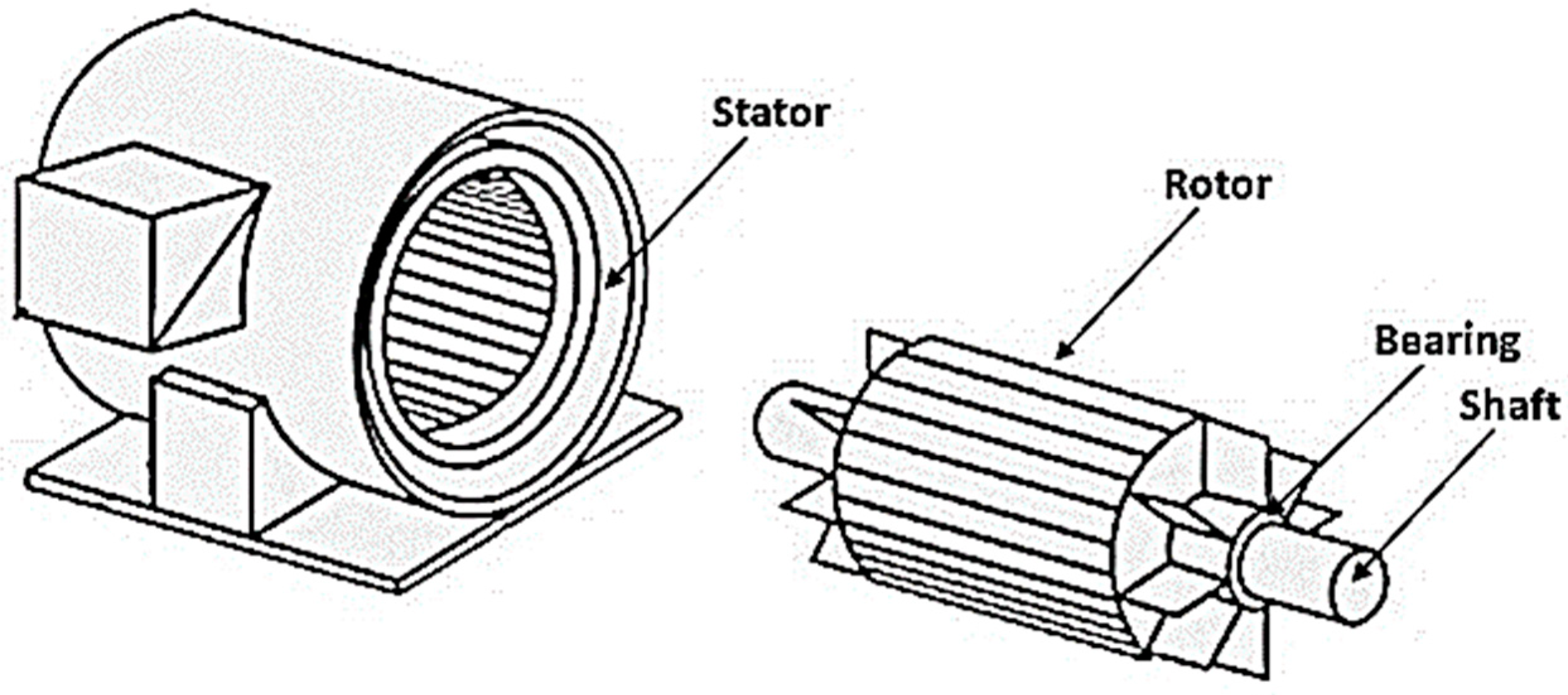
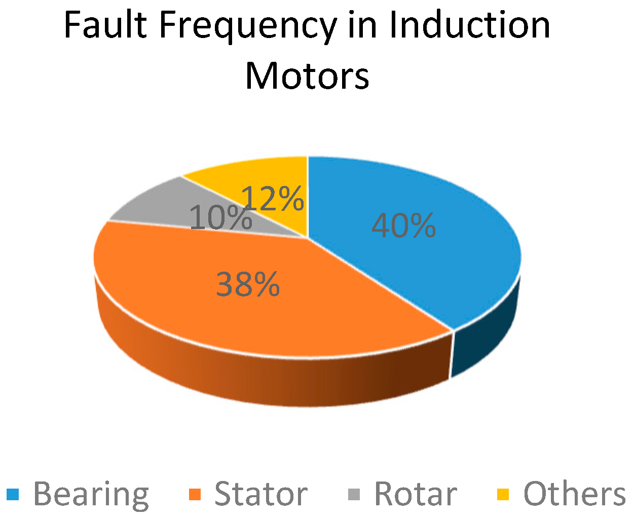
2.1. Condition Monitoring in Electric Motors
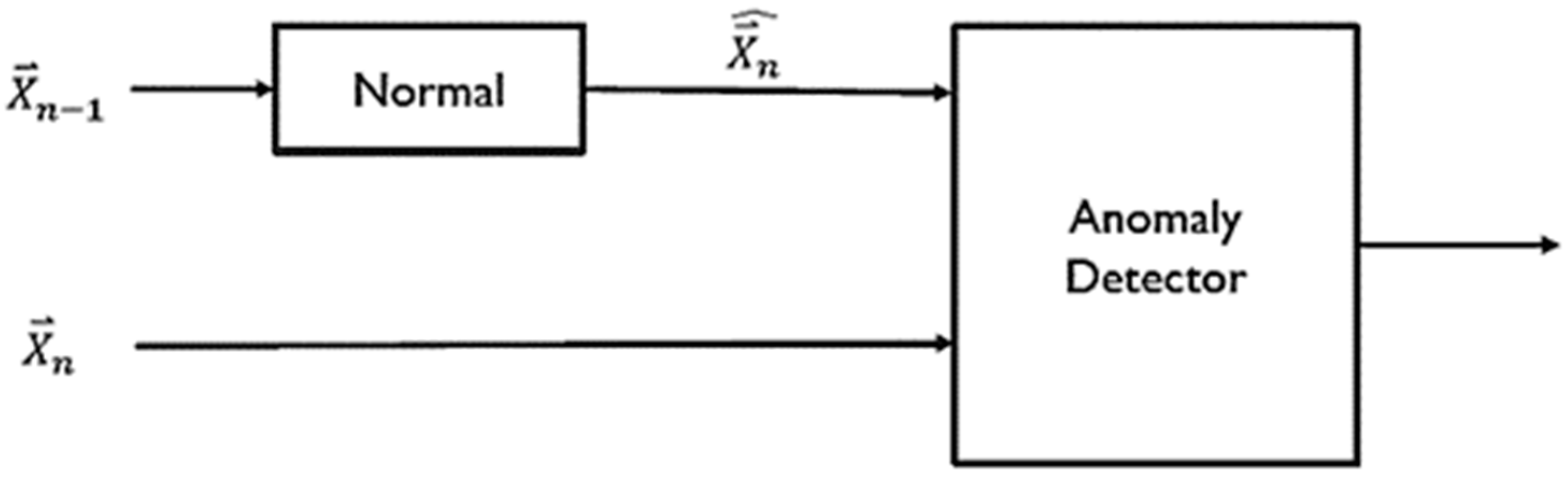
2.2. Anomaly Detection and Deep Learning
3. Data Collection and Dataset Generation
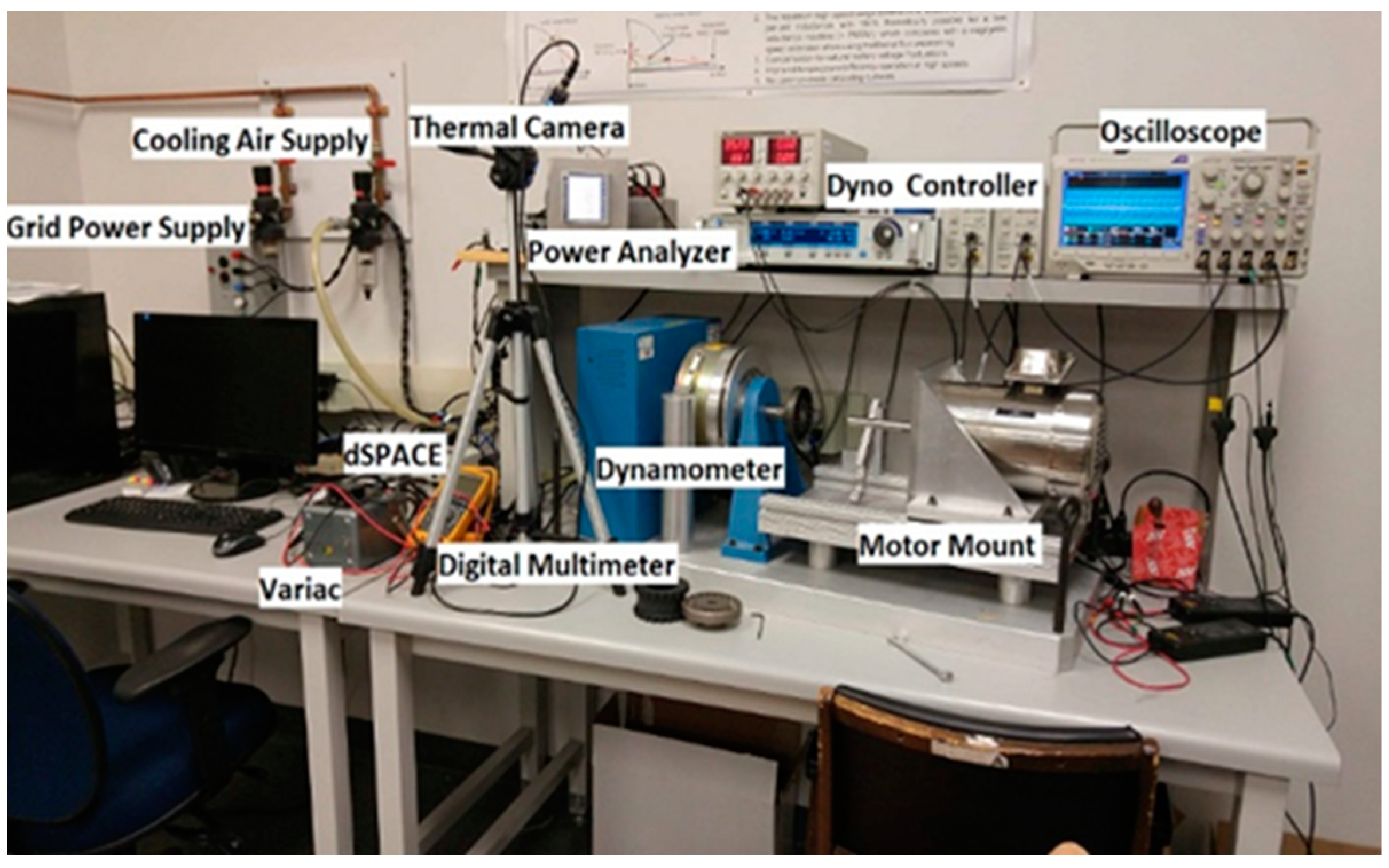
3.1. Hardware and Instruments
3.2. Controlled Variables
3.3. Experimental Design
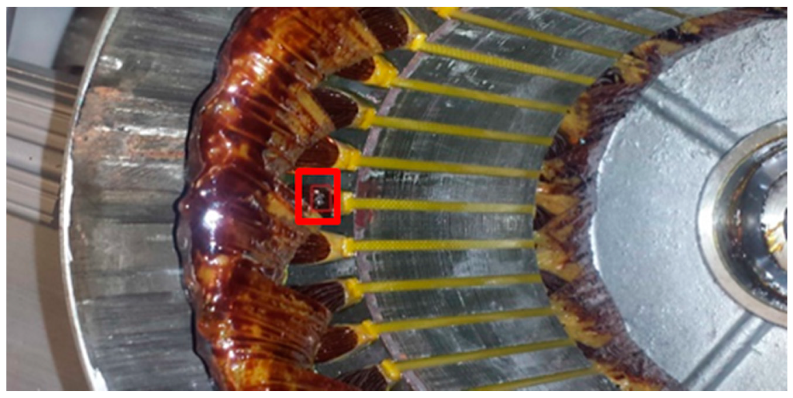
3.3.1. Stator Short
3.3.2. Bearing Faults
- Foreign materials entering the bearing and causing increased wear and pitting on the balls, cage, and inner or outer tracks.
- Under-greasing, or not putting any grease in the bearing, which could cause the bearing to overheat. This could cause the bearings and tracks to deform or warp if they are too hot under load or are going through multiple heating and cooling phases.
- Over-greasing the bearing, causing the seal to be broken, which subsequently causes all of the grease to leak out. This would lead to the same problem as under-greasing the bearing.
- Unbalanced loads on the motor can cause one side of the bearing to wear at a much greater rate than another side, which can lead to static eccentricity.
- Simple friction wear caused by running the motor over many working hours.
- To simulate foreign materials entering the bearing and causing increased wear and pitting, multiple silica carbide beads were packed into the bearing. The bearing was then run on a lathe with the outer ring held stationary at 150 rpm for 40 min. As a side note, after the bearing was run through a full test with the 2.5 h warming period, it was found that the cage holding the bearing balls in place was broken. This cage was not broken before the test was run. The carbide beads were not extensively cleaned out before running the motor for all of its tests, nor was the motor re-greased after the damage was caused.
- To simulate overheating caused by lack of grease, the bearing inner track was heated to a cherry red glow with an acetylene torch. This caused all of the grease to be burned off and left the bearing slightly warped, which caused irregular damage on the inner and outer tracks and the ball bearings. The bearing very clearly ran rough after the damage was caused, and no grease was placed back in the bearing. Running the bearing through the 2.5 h warming period did not seem to cause additional apparent damage.
- The last damage type that was created was a 3 mm hole in the outer track. While this is unlikely to appear in industry, it was completed to compare our results to other research paper’s results as they focused primarily on single point bearing faults, such as a drilled hole in the inner or outer track. The reason they focused on this type of damage is because the damage is supposed to appear at specific frequencies as opposed to general noise increases that random damage causes. Additional bearings were damaged by hitting a bearing’s inner track with a hammer once and multiple times and creating a score on the outer track.
4. Methodology
4.1. Data Preprocessing
4.2. The Condition Monitoring Dataset
4.3. Subsection
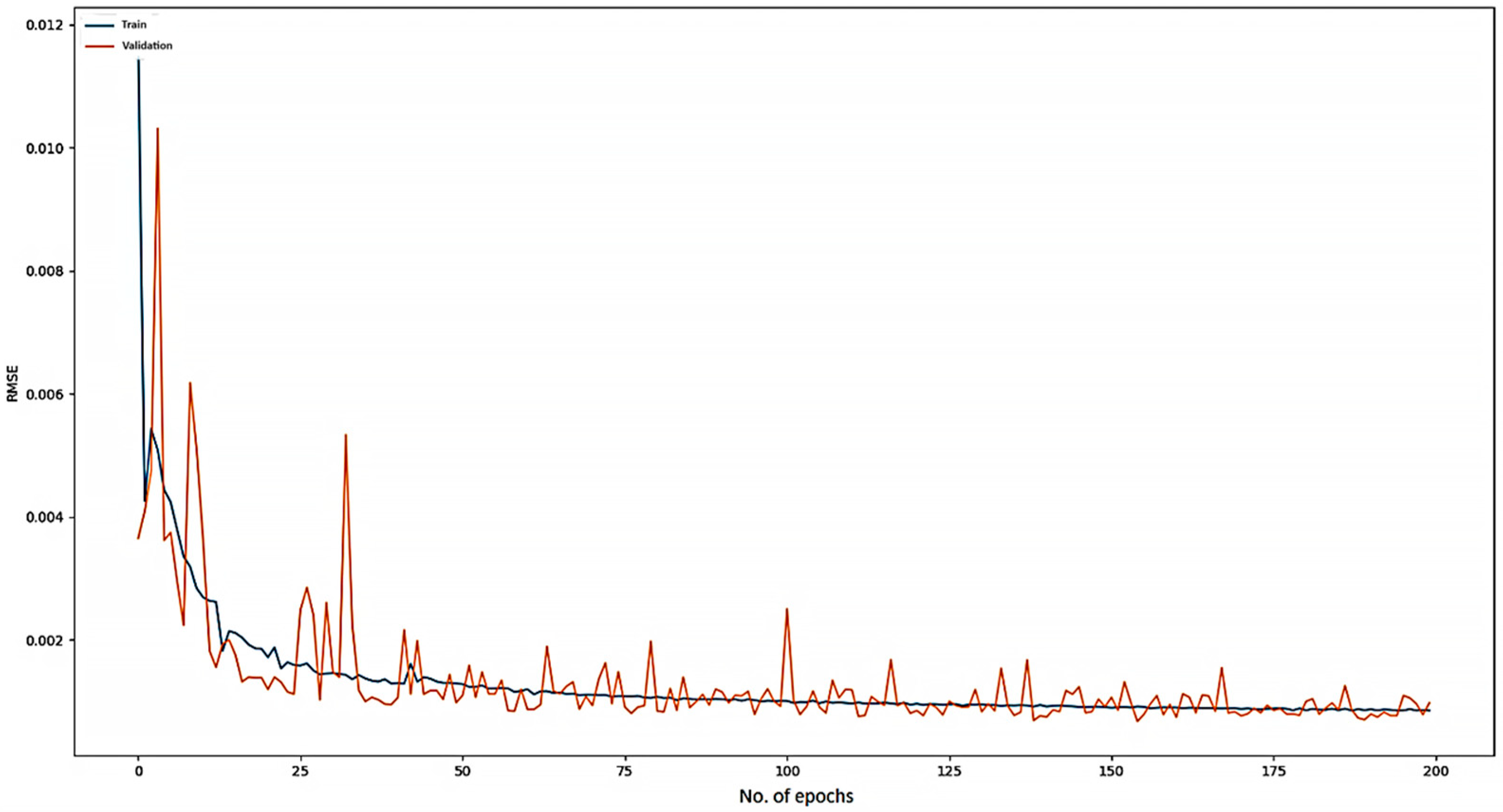
5. Results
6. Summary and Future Work
Author Contributions
Funding
Data Availability Statement
Acknowledgments
Conflicts of Interest
References
- Kim, K.; Parlos, A.G. Induction motor fault diagnosis based on neuropredictors and wavelet signal processing. IEEE/ASME Trans. Mechatron. 2002, 7, 201–219. [Google Scholar]
- Carden, E.P.; Fanning, P. Vibration based condition monitoring: A review. Struct. Health Monit. 2004, 3, 355–377. [Google Scholar] [CrossRef]
- Brosilow, C.; Tong, M. Inferential control of processes. AIChE J. 1978, 24, 485–509. [Google Scholar] [CrossRef]
- Jutan, A.J.M.; Wright, J. Multivariable computer control of a butane hydrogenlysis reactor, part II—data collection, parameter estimation, and stochastic disturbance identification. AIChE J. 1977, 23, 453–464. [Google Scholar]
- Qin, S.J.; Yue, H.; Dunia, R. Self-validating inferential sensors with application to air emission monitoring. Ind. Eng. Chem. Res. 1997, 36, 1675–1685. [Google Scholar] [CrossRef]
- Booth, C.; McDonald, J.R. The use of artificial neural networks for condition monitoring of electrical power transformers. Neurocomputing 1998, 23, 97–109. [Google Scholar] [CrossRef]
- Kamohara, H.; Takinami, A.; Takeda, M.; Kano, M.; Hasebe, S.; Hashimoto, I. Product quality estimation and operating condition monitoring for industrial ethylene fractionator. J. Chem. Eng. Jpn. 2004, 37, 422–428. [Google Scholar] [CrossRef]
- Lamberson, R.E. Apparatus and Method for the Remote Monitoring of Machine Condition. Google Patents US6489884B1, 3 December 2002. [Google Scholar]
- Daroogheh, N.; Baniamerian, A.; Meskin, N.; Khorasani, K. Prognosis and health monitoring of nonlinear systems using a hybrid scheme through integration of PFs and neural networks. IEEE Trans. Syst. Man Cybern. Syst. 2016, 47, 1990–2004. [Google Scholar] [CrossRef]
- Henriquez, P.; Alonso, J.B.; Ferrer, M.A.; Travieso, C.M. Review of Automatic Fault Diagnosis Systems Using Audio and Vibration Signals. IEEE Trans. Syst. Man Cybern. Syst. 2014, 44, 642–652. [Google Scholar] [CrossRef]
- Wu, S.-J.; Gebraeel, N.; Lawley, M.A.; Yih, Y. A neural network integrated decision support system for condition-based optimal predictive maintenance policy. IEEE Trans. Syst. Man Cybern. Part A Syst. Hum. 2007, 37, 226–236. [Google Scholar] [CrossRef]
- Chandola, V.; Banerjee, A.; Kumar, V. Anomaly detection: A survey. ACM Comput. Surv. (CSUR) 2009, 41, 1–58. [Google Scholar] [CrossRef]
- Jawadekar, A.; Paraskar, S.; Jadhav, S.; Dhole, G. Artificial neural network-based induction motor fault classifier using continuous wavelet transform. Syst. Sci. Control Eng. Open Access J. 2014, 2, 684–690. [Google Scholar] [CrossRef]
- Bonaldi, E.L.; de Oliveira, L.E.d.L.; da Silva, J.G.B.; Lambert-Torresm, G.; da Silva, L.E.B. Predictive maintenance by electrical signature analysis to induction motors. In Induction Motors-Modelling and Control; IntechOpen: London, UK, 2012. [Google Scholar]
- Gupta, K.; Kaur, A. A review on fault diagnosis of induction motor using artificial neural networks. Int. J. Sci. Res. 2014, 3, 680–684. [Google Scholar]
- Jaros, R.; Byrtus, R.; Dohnal, J.; Danys, L.; Baros, J.; Koziorek, J.; Zmij, P.; Martinek, R. Advanced Signal Processing Methods for Condition Monitoring. Arch. Comput. Methods Eng. 2023, 30, 1553–1577. [Google Scholar] [CrossRef]
- Nandi, S.; Toliyat, H.A.; Li, X. Condition monitoring and fault diagnosis of electrical motors—A review. IEEE Trans. Energy Convers. 2005, 20, 719–729. [Google Scholar] [CrossRef]
- Zamudio-Ramirez, I.; Osornio-Rios, R.A.; Antonino-Daviu, J.A.; Razik, H.; de Jesus Romero-Troncoso, R. Magnetic Flux Analysis for the Condition Monitoring of Electric Machines: A Review. IEEE Trans. Ind. Inform. 2022, 18, 2895–2908. [Google Scholar] [CrossRef]
- Gurusamy, V.; Capolino, G.-A.; Akin, B.; Henao, H.; Romary, R.; Pusca, R. Recent Trends in Magnetic Sensors and Flux-Based Condition Monitoring of Electromagnetic Devices. IEEE Trans. Ind. Appl. 2022, 58, 4668–4684. [Google Scholar] [CrossRef]
- Tiboni, M.; Remino, C.; Bussola, R.; Amici, C. A Review on Vibration-Based Condition Monitoring of Rotating Machinery. Appl. Sci. 2022, 12, 944–971. [Google Scholar] [CrossRef]
- Kumar, R.R.; Andriollo, M.; Cirrincione, G.; Cirrincione, M.; Tortella, A. A Comprehensive Review of Conventional and Intelligence-Based Approaches for the Fault Diagnosis and Condition Monitoring of Induction Motors. Energies 2022, 15, 8931–8936. [Google Scholar] [CrossRef]
- Trachi, Y.; Elbouchikhi, E.; Choqueuse, V.; Benbouzid, M.E.H. Induction machines fault detection based on subspace spectral estimation. IEEE Trans. Ind. Electron. 2016, 63, 5641–5651. [Google Scholar] [CrossRef] [Green Version]
- Asad, B.; Vaimann, T.; Belahcen, A.; Kallaste, A.; Rassõlkin, A.; Ghafarokhi, P.S.; Kudelina, K. Transient Modeling and Recovery of Non-Stationary Fault Signature for Condition Monitoring of Induction Motors. Appl. Sci. 2021, 11, 2801–2817. [Google Scholar] [CrossRef]
- Qi, R.; Zhang, J.; Spencer, K. A Review on Data-Driven Condition Monitoring of Industrial Equipment. Algorithms 2023, 16, 9. [Google Scholar] [CrossRef]
- Sun, J.; Chai, Y.; Su, C.; Zhu, Z.; Luo, X. BLDC motor speed control system fault diagnosis based on LRGF neural network and adaptive lifting scheme. Appl. Soft Comput. 2014, 14, 609–622. [Google Scholar] [CrossRef]
- Ince, T.; Kiranyaz, S.; Eren, L.; Askar, M.; Gabbouj, M. Real-time motor fault detection by 1-D convolutional neural networks. IEEE Trans. Ind. Electron. 2016, 63, 7067–7075. [Google Scholar] [CrossRef]
- Li, K.; Wang, Q. Study on signal recognition and diagnosis for spacecraft based on deep learning method. In Proceedings of the 2015 Prognostics and System Health Management Conference (PHM), Coronado, CA, USA, 18–24 October 2015; p. 5. [Google Scholar]
- Reddy, K.K.; Sarkar, S.; Venugopalan, V.; Giering, M. Anomaly detection and fault disambiguation in large flight data: A multi-modal deep auto-encoder approach. In Proceedings of the Annual Conference of the Prognostics and Health Management Society, Denver, CO, USA, 3–6 October 2016. [Google Scholar]
- Sun, W.; Shao, S.; Zhao, R.; Yan, R.; Zhang, X.; Chen, X. A sparse auto-encoder-based deep neural network approach for induction motor faults classification. Measurement 2016, 89, 171–178. [Google Scholar] [CrossRef]
- Alvarado-Hernandez, A.I.; Zamudio-Ramirez, I.; Jaen-Cuellar, A.Y.; Osornio-Rios, R.A.; Donderis-Quiles, V.; Antonino-Daviu, J.A. Infrared Thermography Smart Sensor for the Condition Monitoring of Gearbox and Bearings Faults in Induction Motors. Sensors 2022, 22, 6030–6071. [Google Scholar] [CrossRef]
- Rayhan, F.; Shaurov, M.S.; Khan, M.A.N.; Jahan, S.; Zaman, R.; Hasan, M.Z.; Rahman, T.; Bhuiyan, E.A. A Bi-directional Temporal Sequence Approach for Condition Monitoring of Broken Rotor Bar in Three-Phase Induction Motors. In Proceedings of the 2023 International Conference on Electrical, Computer and Communication Engineering (ECCE), Chittagong, Bangladesh, 23–25 February 2023; p. 6. [Google Scholar]
- Pang, G.; Shen, C.; Cao, L.; Hengel, A.V.D. Deep learning for anomaly detection: A review. arXiv 2020, arXiv:2007.02500. [Google Scholar] [CrossRef]
- Chalapathy, R.; Chawla, S. Deep learning for anomaly detection: A survey. arXiv 2019, arXiv:1901.03407. [Google Scholar]
- Perera, P.; Patel, V.M. Learning deep features for one-class classification. IEEE Trans. Image Process. 2019, 28, 5450–5463. [Google Scholar] [CrossRef] [Green Version]
- Blanchard, G.; Lee, G.; Scott, C. Semi-supervised novelty detection. J. Mach. Learn. Res. 2010, 11, 2973–3009. [Google Scholar]
- Goldstein, M.; Uchida, S. A comparative evaluation of unsupervised anomaly detection algorithms for multivariate data. PLoS ONE 2016, 11, e0152173. [Google Scholar] [CrossRef] [PubMed] [Green Version]
- Ruff, L.; Vandermeulen, R.; Goernitz, N.; Deecke, L.; Siddiqui, S.A.; Binder, A.; Müller, E.; Kloft, M. Deep one-class classification. In Proceedings of the International Conference on Machine Learning, Stockholm, Sweden, 10–15 July 2018; pp. 4393–4402. [Google Scholar]
- Chalapathy, R.; Menon, A.K.; Chawla, S. Anomaly detection using one-class neural networks. arXiv 2018, arXiv:1802.06360. [Google Scholar]
- Zheng, P.; Yuan, S.; Wu, X.; Li, J.; Lu, A. One-class adversarial nets for fraud detection. In Proceedings of the AAAI Conference on Artificial Intelligence, Hilton, HI, USA, 27 January–1 February 2019; pp. 1286–1293. [Google Scholar]
- Dai, Z.; Yang, Z.; Yang, F.; Cohen, W.W.; Salakhutdinov, R.R. Good semi-supervised learning that requires a bad gan. In Proceedings of the Advances in Neural Information Processing Systems, Long Beach, CA, USA, 4–9 December 2017; pp. 6510–6520. [Google Scholar]
- Hill, D.J.; Minsker, B.S. Anomaly detection in streaming environmental sensor data: A data-driven modeling approach. Environ. Model. Softw. 2010, 25, 1014–1022. [Google Scholar] [CrossRef]
- Kantz, H.; Schreiber, T. Nonlinear Time Series Analysis; Cambridge University Press: Cambridge, UK, 2004; Volume 7. [Google Scholar]
- Takens, F. Detecting strange attractors in turbulence. In Dynamical Systems and Turbulence, Warwick 1980; Springer: Berlin/Heidelberg, Germany, 1981; pp. 366–381. [Google Scholar]
- Hegger, R.; Kantz, H.; Schreiber, T. Practical implementation of nonlinear time series methods: The TISEAN package. Chaos Interdiscip. J. Nonlinear Sci. 1999, 9, 413–435. [Google Scholar] [CrossRef] [PubMed] [Green Version]
- Yazdanbakhsh, O. Applications of Complex Fuzzy Sets in Time-Series Prediction. Ph.D. Thesis, University of Alberta, Edmonton, AB, Canada, 2017. [Google Scholar]
- Abarbanel, H.; Gollub, J. Analysis of observed chaotic data. Phys. Today 1996, 49, 81. [Google Scholar] [CrossRef]
- Kennel, M.B.; Brown, R.; Abarbanel, H.D. Determining embedding dimension for phase-space reconstruction using a geometrical construction. Phys. Rev. A 1992, 45, 3403. [Google Scholar] [CrossRef] [Green Version]
- Haykin, S.S. Neural Networks and Learning Machines/Simon Haykin; Prentice Hall: New York, NY, USA, 2009. [Google Scholar]
- Witten, I.H.; Frank, E.; Trigg, L.E.; Hall, M.A.; Holmes, G.; Cunningham, S.J. Data Mining: Practical Machine Learning Tools and Techniques, 4th ed.; Morgan Kaufmann: Burlington, MA, USA, 2016. [Google Scholar]
- Chollet, F. Deep Learning with Python; Manning Pub. Co.: Shelter Island, NY, USA, 2018. [Google Scholar]
- Fukushima, K. Neocognitron: A self-organizing neural network model for a mechanism of pattern recognition unaffected by shift in position. Biol. Cybern. 1979, 36, 193–202. [Google Scholar] [CrossRef]
- Jain, R.; Kasturi, R.; Schunck, B.G. Machine Vision; McGraw-Hill: New York, NY, USA, 1995. [Google Scholar]
- Breiman, L.; Friedman, J.; Stone, C.J.; Olshen, R.A. Classification and Regression Trees; CRC Press: Boca Raton, FL, USA, 1984. [Google Scholar]
- Breiman, L. Random forests. Mach. Learn. 2001, 45, 5–32. [Google Scholar] [CrossRef] [Green Version]
- Pedregosa, F.; Varoquaux, G.; Gramfort, A.; Michel, V.; Thirion, B.; Grisel, O.; Blondel, M.; Prettenhofer, P.; Weiss, R.; Dubourg, V. Scikit-learn: Machine learning in Python. J. Mach. Learn. Res. 2011, 12, 2825–2830. [Google Scholar]
- LeCun, Y.; Bengio, Y.; Hinton, G. Deep learning. Nature 2015, 521, 436–444. [Google Scholar] [CrossRef]
- Osornio-Rios, R.A.; Zamudio-Ramírez, I.; Jaen-Cuellar, A.Y.; Antonino-Daviu, J.; Dunai, L. Data Fusion System for Electric Motors Condition Monitoring: An Innovative Solution. IEEE Ind. Electron. Mag. 2023, in press. [Google Scholar] [CrossRef]


| Number of Clusters | Standard Deviation | Train RMSE | Validation RMSE |
|---|---|---|---|
| 100 | 10−5 | 0.0323 | 0.0766 |
| Model | TPR | FPR | Accuracy |
|---|---|---|---|
| MLP | 0.947 | 0.366 | 0.791 |
| RBF | 0.918 | 0.085 | 0.912 |
| Decision Tree | 0.967 | 0.207 | 0.881 |
| Random Forest | 0.993 | 0.264 | 0.864 |
| Model | TPR | FPR | Accuracy |
|---|---|---|---|
| MLP (12 Inputs) | 0.732 | 0.166 | 0.824 |
| MLP (18 Inputs) | 0.795 | 0.129 | 0.861 |
| Decision Tree (12 Inputs) | 0.944 | 0.037 | 0.956 |
| Decision Tree (18 Inputs) | 0.748 | 0.162 | 0.811 |
| Random Forest (12 Inputs) | 0.948 | 0.033 | 0.968 |
| Random Forest (18 Inputs) | 0.841 | 0.101 | 0.895 |
Disclaimer/Publisher’s Note: The statements, opinions and data contained in all publications are solely those of the individual author(s) and contributor(s) and not of MDPI and/or the editor(s). MDPI and/or the editor(s) disclaim responsibility for any injury to people or property resulting from any ideas, methods, instructions or products referred to in the content. |
© 2023 by the authors. Licensee MDPI, Basel, Switzerland. This article is an open access article distributed under the terms and conditions of the Creative Commons Attribution (CC BY) license (https://creativecommons.org/licenses/by/4.0/).
Share and Cite
Sobhi, S.; Reshadi, M.; Zarft, N.; Terheide, A.; Dick, S. Condition Monitoring and Fault Detection in Small Induction Motors Using Machine Learning Algorithms. Information 2023, 14, 329. https://doi.org/10.3390/info14060329
Sobhi S, Reshadi M, Zarft N, Terheide A, Dick S. Condition Monitoring and Fault Detection in Small Induction Motors Using Machine Learning Algorithms. Information. 2023; 14(6):329. https://doi.org/10.3390/info14060329
Chicago/Turabian StyleSobhi, Sayedabbas, MohammadHossein Reshadi, Nick Zarft, Albert Terheide, and Scott Dick. 2023. "Condition Monitoring and Fault Detection in Small Induction Motors Using Machine Learning Algorithms" Information 14, no. 6: 329. https://doi.org/10.3390/info14060329